Sage Journals: Discover world-class research

Abstract

Identification of molecular-based signatures is one of the critical steps toward finding therapeutic targets in cancer. In this paper, we propose methods to discover prognostic gene signatures under a causal structure learning framework across the whole genome. The causal structures are represented by directed acyclic graphs (DAGs), wherein we construct gene-specific network modules that constitute a gene and its corresponding regulators. The modules are then subsequently used to correlate with survival times, thus, allowing for a network-oriented approach to gene selection to adjust for potential confounders, as opposed to univariate (gene-by-gene) approaches. Our methods are motivated by and applied to a clear cell renal cell carcinoma (ccRCC) study from The Cancer Genome Atlas (TCGA) where we find several prognostic genes associated with cancer progression - some of which are novel while others confirm existing findings.

Keywords

kidney cancer Markov equivalence class network Peter and Clark (PC) algorithm survival time

Introduction

The most common and most lethal type of kidney cancer or renal cell carcinoma (RCC) is clear cell renal cell carcinoma (ccRCC).¹ Much heterogeneity exists within the ccRCC subtype of kidney cancer, and various factors are used to characterize the disease. This includes disease stage, tumor size, tumor cell morphology, lymph node status, and patient response to treatment.² The Cancer Genome Atlas (TCGA) ccRCC study³ used multiple platforms to determine the associations between the molecular signatures of the disease and patient survival. These analyses identified a role for the PI(3) K/AKT pathways in tumorigenesis and ccRCC progression, and therefore as therapeutic targets.

The goal of this paper is to find gene signatures that are associated with patients' survival times. Based on the understanding of most disease processes, the ccRCC phenotype does not result from a mutation in a single gene, but rather from a coordinated series of interactions involving multiple molecular pathways and multiple genes.⁴ Our main hypothesis is that genes influencing patient's survival times are cumulative effects of a given gene as well as its (upstream) regulators. The main goals of this study are (1) to determine the whole genome causal network from gene expression data and (2) to relate each gene expression to patient survival, adjusting for the estimated causal network (hence, regulators). The incorporation of analytic methods that are based on network models of gene expression has improved our ability to identify elements that can serve as biomarkers of patient prognosis. Because the interactions between the expressions of different genes are assessed within a biological network, this construct is labeled as a gene co-expression network. In a layout of this network, the gene functions are shown as vertices and the significant associations between gene functions are shown as connections (or edges) between them.⁵ All edges in a co-expression network are undirected and can be quantified by different statistical measures, such as marginal correlations, partial correlations, or mutual information.⁶ In existing approaches, there are two main aspects of gene co-expression networks: (1) hub genes and (2) modularity. In a co-expression network that corresponds to a set of genes, hub genes are the genes that connect to a significant proportion of the total genes in the network. In contrast, a modularity approach focuses on a subnetwork that has a higher density of edges within groups of genes than between them. Recent works, such as Han et al.⁷, Taylor et al.⁸, Patel et al.⁹, and Yang et al.¹⁰, uncovered prognostic genes for an outcome variable based on the characteristics of genes in the co-expression network.

Although the undirected co-expression network estimated from observational gene expression data has been useful to select prognostic genes, they do not explicitly account for directionality of the mechanistic regulation between the genes. The delineation of causal (directed) relations among genes would be useful not only in discovering (upstream) regulators for a particular gene but also in identification of predictive gene signatures involved in cancer progression. Causal relationships can be concisely represented by directed acyclic graph (DAG) models, and given an estimated/known DAG model, the causal effects can be computed using standard methods as in Pearl.¹¹

However, a DAG model is not directly identifiable (in a statistical sense) from observational/static gene expression data. Maathuis et al.¹², proposed a method called IDA (intervention-calculus when the DAG is absent) to infer bounds on total causal effects under a limited causal structure estimated from observational data. Motivated by the IDA method, we propose methods to rank genes based on their effects on patient survival times, adjusting for their causal structure, ie, regulators. Our method has two main steps: estimating the causal structure of genes that identifies network modules for each gene and its regulators (“parents”), and then, subsequently, using the modules consisting of a gene and its parents to estimate the effects on survival times. In essence, this constitutes a network-oriented method as opposed to univariate gene analyses - thus, refining the estimations since it adjusts for potential confounders (as we demonstrate in the sequel).

The most challenging part of this analysis is to estimate the causal structure for a large number of genes (typically on the order of 10⁴). IDA starts from a completely connected graph in which all pairs of genes are connected and iteratively removes the edges (“thins the graph”) by excluding edges with all orders of conditional independences (marginal independence, first-order conditional independence, and so on). However, to exclude an edge, the set of variables (conditioned on) needs to be a set of all subsets of the inter-connected variables – which leads to an exhaustive search over the large number of edges and vertices. Using penalized regression technique, we estimate sparse graphical models and use algorithms based on IDA to estimate the causal structure – thus, enabling us to scale our methods to such high-dimensional genomics data. Applying our methodology to TCGA ccRCC tumor samples, we found significant gene modules in ETS and Notch family. The signatures also involve the genes ARID1A and SMARCA4, which were found by the TCGA Research Network's study of ccRCC.³

In Section 2, we introduce and describe our methodology. In Section 3, we present the results of the analysis of TCGA data to select prognostic gene signatures for the survival time of patients with ccRCC. In Section 4, we provide a summary and discussion.

Methods

We propose an approach for estimating the effect of each gene on patient survival, adjusted for the causal structure of all the genes of interest. The causal structure forms modules for each gene that consists of a gene and its parents - where parents are defined by the set of genes having a directed edge (pointing) toward a gene in a graph. The main challenge is that the unique determination of modules is unidentifiable from observational gene expression data. To address this issue, we propose a principled statistical procedure that consists of two main parts: (1) estimating the causal structure, which includes direct and indirect relations among genes, for high-dimensional gene expression data and (2) evaluating the effects of each gene under the ambiguous causal structure. Figure 1 concisely describes the entire workflow of our method. Briefly, the causal structure is first estimated through several undirected/partially directed graphs from Steps 1 to 6 and the edges are sequentially thinned with different implications of the dependencies for edges in different graphs. The eventual causal structure represented by the completed, partially directed acyclic graph (CPDAG) in Step 6 includes undirected edges when the directions are not identifiable. To address the issue of identifiability, several effect sizes of each gene for all possible modules from the CPDAG are obtained by the Cox-proportional hazards model, and the minimum effect size is used for ranking the genes. As opposed to the single gene analysis, we refine the estimation of effect size based on the estimated causal structure and show how this leads to better quantification of the prognostic effects. In the following subsections, we describe in detail our method for the causal structure estimation and the effect size evaluation given the causal structure.

Figure 1.

Workflow to obtain the whole genome causal structure: pairs of genes (edges) are sequentially excluded by conditional (marginal) independence tests, starting from a completely connected graph and arriving at a skeleton. V-structure detection and completion steps then follow. PDAG is partially directed acyclic graph and CPDAG is completed PDAG.

Estimation of the causal structure for genes

We study the causal relations of p variables X₁, …, X_p by a DAG G = (V, E) with a set of vertices V = {1, …, p} and a set of edges E ⊆ V × V. All edges in the DAG are directed; in that, (v, w) ∈ E but (w, v) ∉ E for all v ∈ V ≠ w ∈ V. The acyclic graph means that the DAG contains no cycle (no path from a vertex to the same vertex along with directed edges). In our context, the vertices/variables represent genes, and the edges represent directed relations between pairs of these genes. We assume that X = (X₁, …, X_p)^T ∈ R^p follows a multivariate normal distribution N_p(0, Σ) with the density function f_Σ(·). The parent vertices of a vertex i ∈ V are defined by the vertices pointing toward the vertex i. We denote the parent vertices of i ∈ V by pa_i, and the corresponding variables by X_pa. The Markov properties determined by the DAG G admit recursive factorization of the joint probability density function f_Σ,

f_{\sum} (X_{1}, \dots X_{p}) = \prod_{i = 1}^{p} f (X_{i} | X_{p a_{i}})

The joint distribution of X is decomposed into conditional densities of each variable given its parents. Because several different DAGs may determine the same factorization, the DAG G is not identifiable from the observational distribution. The Markov property on the observational distribution of X provides the relations of conditional independence among the random variables. However, a collection of all the DAGs that correspond to the same set of conditional independence restrictions can be assembled into a Markov equivalence class, which can be determined based on observational data.

The approaches described by Spirtes et al.¹³, and Pearl¹¹ rely on a series of conditional independence tests to estimate a Markov equivalence class. The framework of the inductive causation (IC) algorithm is based on the theorem in Andersson et al.¹⁴: two DAGs are Markov equivalent if and only if they have the same skeleton and the same v-structures. The skeleton of a DAG G is obtained by replacing all directed edges with undirected edges. A v-structure is an ordered triplet of vertices (i, j, k) such that G contains the directed edges (i, k) ∈ E and (j, k) ∈ E and (i, j) ∉ E (i → k ← j). From the observational distribution, the skeleton and v-structures can be identified and are represented by a partially directed acyclic graph (PDAG). The undirected edges in the skeleton and the directions present in the v-structures imply conditional independencies among the variables corresponding to V:

There is an edge between vertices i and j in the skeleton if and only if the variables X_i and X_j are dependent, conditional on variables corresponding to X_S = {X_k: k ∈ S} for all S ⊆ V\{i, j}.

In a v-structure i → k ← j, X_i and X_j are dependent, conditional on every set that contains X_k or its descendants.

The framework of the IC algorithm¹¹ relies on the conditional independence constraint and consists of three steps: (1) estimation of the skeleton by conditional independence tests, (2) identification of the v-structures, and (3) completion of the PDAG obtained from (1) and (2). We follow the framework of the IC algorithm by modifying the details of the algorithms to be suitable for high-dimensional data. We describe each step of our method in the following subsection.

Estimation of the skeleton. Spirtes et al.¹³, described various algorithms for estimating the skeleton. Our method is a modification of the standard algorithm known as the Peter and Clark (PC) algorithm, which has been shown to be consistent for high-dimensional sparse graphs.¹⁵ The modification of the PC algorithm is based on the concept of a moral graph of a DAG. Given a DAG G, moralization of a DAG is executed by connecting the vertices i and j that form a v-structure i → k ← j, and replacing all directed edges by undirected edges. This moral graph is a Gaussian graphical model (GGM) that is specified by the structure of zeros in the inverse covariance matrix Σ⁻¹.¹⁶ The PenPC algorithm¹⁷ starts from a GGM instead of a completely connected graph in the PC algorithm. The PenPC algorithm uses penalized regressions to estimate the GGM, which allows for the removal of a large amount of edges from the initial stage. The sparsity of the GGM makes skeleton estimation feasible for high-dimensional data, such as our ccRCC gene expression data, with p = 14,576. Motivated by the PenPC algorithm, the estimation of the skeleton proceeds in two stages: (1) the GGM is estimated based on penalized full-order partial correlations and (2) more edges in the GGM are removed by lower order (unpenalized) partial correlation tests. From a known DAG, G = (V, E), we can construct the GGM by the moralization and the skeleton by replacing the directed edges with undirected edges. We denote the GGM and the skeleton of the DAG, G = (V, E), by G^m = (V, E^m) and G^u = (V, E^u) with superscripts. The edges in E^m and E^u are all undirected, which means that (i, j) ∈ E^u (j, i) ∈ E^u. In an undirected graph, the neighborhood of a vertex v is defined by the set of vertices that are connected to v. Note that l-order conditional independence means that conditional independence exists between two variables given l number of variables. The conditional independence is assessed by estimated partial correlations ${\hat{ρ}}_{i j | S}$ between X_i and X_j given a subset of other variables ${X_{k} : k \in S \subseteq V \ {i, j}}$ . For test statistics, we calculate the Z-transformed partial correlations, $z_{i j | s} = (1 / 2) \log (1 + {\hat{ρ}}_{i j | s} / 1 - {\hat{ρ}}_{i j | s}),$ , and reject the null hypothesis if $|_{z i j | s |} \sqrt{n - | s | - 3 |} > Φ^{- 1} (1 - α / 2),$ , where Φ is the standard normal distribution function and 0 < α < 1 is the P-value cutoff. Hereafter, we provide the details of the algorithm.

[Step 1] Estimation of the GGM, Gm = (V, Em). Meinshausen and Bühlmann¹⁸ proposed a regression-based approach to estimate a GGM. The neighborhood of v is estimated by a penalized regression of the variable corresponding to v versus the remaining variables. After estimating all p penalized p − 1 dimensional coefficients by separate estimations, the graph structure is estimated based on the zero structure of those coefficients. For a response X_v where v ∈ V, we use procedures 1A and 1B, given below:

Procedure 1A. Marginal correlations are calculated between X_v and all other variables, ${X_{w} : w \in v \ {v}} .$ Set ${X_{w} : w \in v \ {v}} .$ if the P-value from the marginal correlation test between X_v and X_w is less than α, which is the P-value cutoff, where ne₀(v) is the set of neighboring vertices of v in the correlation graph.

Procedure 1B. For all X_v, v ∈ V, we select a neighborhood, denoted by ne(v), using a penalized regression with X_v as a response variable and the variables {X_w: w ∈ ne₀(v)} as explanatory variables,

\begin{array}{r} {\hat{β}}_{v} = \underset{β_{v} \in R | n e_{0} (v) |}{\arg \min} \frac{1}{2} {(x_{v} - X_{n e_{0}} (v) β_{v})}^{T} (X_{n e_{0}} (v) β_{v}) + n λ v \\ \sum_{w \in n e_{0} (v)} \log (| β_{v w} | + τ_{v}), \end{array}

where x_v is an n × 1 vector for n measurements of variable X_v and

X_{n e_{0}}

(v) is the n × |ne₀, (v)| matrix for variables

{X_{w} : w \in n e_{0} (v)}

and

β_{v} = {(β_{v 1}, …, β_{v | n e_{0} (v) |})}^{T}

.¹⁷ The tuning parameters, λ_v and τ_v, are selected by using an extended Bayesian information criterion¹⁹ for each regression. From all the estimated regression coefficients {

{\hat{β}}_{v w} : v, w \in V

and

v \neq w

}, we estimate the edge set of the GGM, E^m, by

E^{m} = {(v, w) : β_{v w} \neq 0]} .

In the Step 1 of the PenPC algorithm,¹⁷ they fit the p penalized regressions without marginal independence tests at the beginning; in other words, all regressions involve p − 1 covariates. In this algorithm, we include the neighborhoods from the correlation graph for each response variable as the covariates in the penalized regression corresponding to the response.

[Step 2] Estimation of the skeleton, Gu = (V, Eu). If an edge (v, w) belongs to E^m, which is an edge set of the GGM, the genes X_v and X_w are conditionally dependent given all other genes (full-order conditional independence). An edge (v, w) in a skeleton is equivalent to the variables X_v and X_w, which are conditionally dependent given all subsets of the other variables. Therefore, more edges will be removed from the GGM if any lower order partial correlation test provides a P-value greater than the threshold α. For an edge (v, w) that is in the GGM but removed from the skeleton ((v, w) ∈ E^m and (v, w) ∉ E^u), we calculate a separation set that is the union of the sets that induce conditional independence between the variables X_v and X_w.

Our algorithm performs the partial correlation tests from the first order, l = 1, until l exceeds the maximum size of the neighborhoods in the current graph. We denote ne(i, G) as the set of neighbors for i ∈ V in an undirected graph G. Our algorithm is summarized in detail in Figure 2. It starts from the first-order partial correlation tests because we already tested marginal correlations to estimate the GGM. For a fixed order, l, each edge is tested by partial correlations given the subsets in the neighborhood for either vertex that forms the edge. We changed the order-independent version of the PC algorithm in Colombo et al.²⁰ to an algorithm that can operate in parallel with the vertices and the order l. The main difference between our algorithm and the PC algorithm is in the calculation of the separation sets. While the PC algorithm stops testing an edge when a separation set is obtained, our algorithm exhaustively searches all vertices that participate in any of the separation sets (Step 2.2.1 of Fig. 2). The exhaustive search provides a more accurate estimation of the v-structures.

Figure 2.

A modified PC algorithm starting from a GGM.

v-structure identification. All edges (v, w) ∉ E^u have separation sets denoted by S_vw. Consider a triplet (v, w, k) such that v-k-w in the skeleton. From the conditional independence property of the v-structure, if v → k ← w, k must not be in the separation set S_vw because X_v and X_w are conditionally dependent given any set containing the variable X_k corresponding to the child vertex k. Thus, we direct the triplet as $v \to k \leftarrow w$ if $k \notin S_{v w}$ .

Using all the graphs, the correlation graph, GGM, and skeleton, in our algorithm, we determine the v-structures for the triplets, (v, w, k), such that $(v, k) \in E^{u}, (w, k) \in E^{u}$ , and $(v, k) \notin E^{u}$ . From our method, the edges are sequentially removed, working from a completely connected graph to the correlation graph, from the correlation graph to the GGM, and from the GGM to the skeleton. From the algorithm in Figure 2, we have separation sets S_vw only for edges excluded between the GGM and the skeleton. The separation sets for edges excluded from the correlation graph are empty sets. For edges excluded between the correlation graph and the GGM, the separation sets are all the other variables, ie, V\{v, w} for an edge (v, w). The triplet with (v - k - w) in the skeleton forms a v-structure, v → k ← w, if one of the following conditions (a) or (b) is satisfied:

The edge (v, w) is excluded from the correlation graph.

(i) The edge (v, w) is in the GGM, ie, X_v and X_w are marginally correlated and partially correlated given all other variables ${X_{k} : k \in V \ {v, w}},$ , and (ii) $k \notin S_{v w} .$ .

Using the above rules, we obtain a PDAG that represents the skeleton and v-structures.

Completion of the PDAG. The completion of the PDAG obtained from the skeleton and v-structures is accomplished by maximally orienting the remaining undirected edges, with restrictions of no directed cycle and no extra v-structure. This completion is done by applying several deterministic rules from Meek²¹ and Pearl.¹¹ The resulting graph is called the CPDAG. It represents the Markov equivalence class. The directed edges in the CPDAG exist in every DAG in the equivalent class; otherwise, the directions for the undirected edges in the CPDAG are reversible in some DAGs in the equivalent class.

Selection of gene signatures based on the causal gene modules

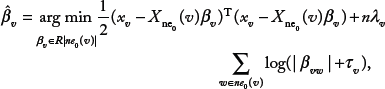
In this section, we identify which genes have a significant effect on survival time. The unsupervised causal structural learning in the previous section provided a CPDAG that represents a Markov equivalence class. The main idea is that when we model a gene in relation to survival time, we adjust for its parent genes, which are obtained from the CPDAG. If the DAG that represents the causal relations for V is known, the parent genes for all vertices are obvious. Using the unique gene modules for each gene, we can obtain the effect of a gene on patient survival by including the expressions of its parent genes in a Cox-proportional hazards model. However, the undirected edges in the CPDAG generate uncertainty in determining the parent genes: the arrows of the undirected edges imply either directions. Similar to the IDA method,¹² our approach accounts for all possible parent genes by switching the directions for the undirected edges and obtains the lower bound for the effect of a gene on survival time.

For a gene i, we define a set of parents {j: j → i} and children {j: j ← i} only for the directed edges. If all neighboring vertices of i are directed, then we have an obvious parent set for i. For an undirected edge that connects to vertex i in the CPDAG, the parents and children are indistinguishable. Under this uncertainty, all effects are computed by switching the directions without creating extra v-structures or cycles on the CPDAG. The detailed algorithm for constructing the candidate set of parents for a vertex is described in Maathuis et al.¹²

Application to Kidney Cancer Data

TCGA ccRcc data description

RNA-seq and clinical data are available in TCGA for 480 patients with primary ccRCC. Among those 480 patients, 343 were censored; the quantiles of the observed survival times in days were 2 (0%), 326.75 (25%), 456.35 (33%), 619.90 (45%), 731.00 (50%), 830.15 (66%), 1,338.50 (75%), and 2,830 (100%). We analyzed RNA-seq V2 data from TCGA tumor tissues for 480 patients with ccRCC (accessed as of November 7, 2013). We filtered out genes with 75 percentiles across the 480 samples less than 25. After removing genes with low expression, we obtained 14,576 genes that are used for downstream analyses. The expression of each gene within each sample is measured by total read counts. We used log₁₀ transformed total read counts in this study. We obtained a 480 × 14,576 residual dataset after removing the effects of several batch covariates by linear regression: 75th percentile of log₁₀ total read counts, capturing the read depth for each sample, plate, and institution. Then we standardized the residual data to have a mean of zero and a unit variance for each gene. The final expression values conform very well with the normal distribution (Fig. 3) - thus, facilitating GGM approaches.

Figure 3.

The histogram of the post-processed expressions. The standard normal density curve is overlaid on the histogram.

From unsupervised learning, we estimated a whole genome expression network, that is a CPDAG in which some of the edges are directed, with the set of vertices V = {1, …, 14,576}. Then we evaluated the effect of each gene in V by using a Cox-proportional hazards model, adjusting for the causal structure, CPDAG. The PC algorithm implemented in the pcalg package of Kalisch and Bühlmann¹⁵ and Colombo and Maathuis²⁰ is not applicable for estimating a skeleton for the number of vertices we analyzed, P = 14,576. Thus, at the beginning of the PC algorithm, we used penalized regressions, which are more suitable for these high-dimensional data. Based on the estimated causal structure for the genes, we evaluated the effect of each gene on survival time. We describe the details of the CPDAG estimation results in the Appendix.

Results

Using graph theory terminology, we refer to “parent” (“child”) genes as genes pointing toward (away from) the gene of interest.

Gene rankings: Our gene ranking is based on the Cox-proportional hazards model, adjusted for the estimated CPDAG and four clinical covariates: patient age and tumor stage, grade, and metastasis status. We refer to this model as the network-adjusted model. To benchmark our method, we considered the model that includes the gene expression and the four clinical covariates with no parent gene and refer it as the unadjusted model. Therefore, in the network-adjusted model (which includes the set of gene parents for each gene), we have more parameters than the unadjusted model. Figure 4 displays the scatter plot of the effect sizes from the unadjusted model versus the network-adjusted model for all 14,576 genes. The slope of the regression line in the scatter plot was 0.893 with zero intercept. The trend with the slope less than 1 indicates that the effect sizes from the network-adjusted models are overall less than the effect sizes from the unadjusted model. However, the areas, A1 and A2, in Figure 4 indicate that the effect sizes from the network-adjusted model are greater than the maximum in the effect sizes from the unadjusted model. Although the effect sizes from the unadjusted model tend to be greater than those from the network-adjusted model, several genes show evident increases in their effect sizes by adding the set of parent genes (located in the regions A1 and A2). Especially, BAT3 gene showed the sign change in the effect sizes from the unadjusted model (0.04) to the network-adjusted model (-0.5) with 1,136.57% relative increase in their effect sizes by adding the parent genes, BAT2, FLOT1, and NOC2L (Table 1). Both BAT3 and BAT2 genes are HLA-B-associated transcripts, and the sequences of the two genes were shown to be closely linked.²² EEF1A1 gene showed 1,311.37% relative increase in the effect sizes from the unadjusted model to the network-unadjusted model by adjusting for EEF1A1P9 gene (Table 1). The EEF1A1P9 gene is a pseudogene that is a dysfunctional gene with sequence similar to EEF1A1 gene, and has lost their protein-coding ability or is no longer expressed.²³ Regulated by the pseudogene EEF1A1P9, EEF1A1 gene has a significant effect on the survival times. In summary, the top-ranked genes from the network-adjusted model are in the areas A1 and A2 in Figure 4, and this indicates that most of the top-ranked genes are not found in the unadjusted model.

Table 1.

Top 50 genes (for ccRCC), ranked by the network-adjusted model: effects on survival time measured by the network-adjusted model and unadjusted model, relative increase in effect size resulting from the network-adjusted model compared to that from the unadjusted model, parent genes, and children genes. The red and green texts in the third and fourth columns indicate negative and positive effects, respectively.

RANK	GENE	EFFECT (a) (ADJUSTED)	EFFECT (b) (UNADJUSTED)	$\frac{(\| a \| - \| b \|)}{\| b \|} \times 100$	PARENT GENES	CHILDREN GENES
1	TAF6	0.67	0.26	155.61%	COPS6, CUX1, LRWD1, MOSPD3, SNX15, USP21
2	GABBR1	0.64	0.28	124.34%	AGPAT4, C2orf63, CACNB1, EBF4, ZNF767
3	MFAP4	-0.61	-0.11	449.1%	AEBP1, CAPN6, DCN, HSPB6, LOC399959, MAPK7, THBS2
4	MARCKSL1	0.6	0.27	123.32%	FJX1, FSCN1, GABPB1, ITPKB	MDFI, MEX3A, PDE4DIP
5	CAP1	-0.56	-0.17	224.86%	ACTR3, EPB41L2, TPM3	CAPZB, ELOVL1
6	MRPS36	-0.56	-0.21	164.93%	ATP5H, CDK7, COX7C	RUNDC3B
7	IK	-0.55	-0.2	173.38%	AATF, BRD8, HARS	SF3B2, SLC4A1AP, SLU7, SUGT1, ZMAT2
8	PLB1	0.54	0.11	373.35%	CSF1R, IGSF21	SP110
9	IRF1	-0.54	-0.19	175.37%	BATF2, BCL3, C5orf56	TOE1
10	PSMD14	0.53	0.21	151.4%	DPP3, OLA1, PSMA5
11	TMED9	-0.52	-0.16	231.64%	B4GALT7, FAF2, LMAN2, SEC61A1, SIL1
12	FGFR4	0.52	0.05	975.17%	C22orf36, LMAN2, PDZK1, SLC16A4
13	UNG	0.52	0.13	287.44%	ACACB, ESYT1, FBXO21, GALNT4, MRPS23, SNRPF, SPPL3
14	SEMA6B	0.52	0.11	363.7%	CCDC85B, DAPK3, VWF	UPP1
15	PIGU	0.5	0.2	151.9%	ALG8, CSE1L, DYNLRB1, RPN2	TTLL1
16	AZI1	0.5	0.26	94.05%	HDGFRP2, LRRC45	MYO18A
17	SLC30A5	-0.5	-0.15	228.9%	AGGF1, GFM2, GMCL1, HEXB, IPO11, MIER3, NUDT18	UTP15
18	BAT3	-0.5	0.04	1136.57%	BAT2, FLOT1, NOC2L	BTBD9, RNF5, SKIV2L, YIPF3
19	TCF25	-0.49	-0.08	484%	COG4, DNAH14, KATNB1, KLHDC4, TSC2
20	ADAP2	0.49	0.14	248.51%	LCP2	GAL3ST4, LOC93622, RNF135, TMEM106A
21	UBE2L3	0.49	0.11	325.61%	CRKL, DYNLRB1, FBXO7, SNRPD3, TOMM22
22	EEF1A1	-0.48	-0.03	1311.37%	EEF1A1P9	GRIPAP1, LOC644936
23	TTC1	-0.47	-0.24	97.07%	ATP6V0E1, MRPL22, PFDN1, RARS, SLU7	ZMAT2
24	ZSCAN18	0.47	0.03	1319.16%	CLDN3, MTMR4, ZNF135, ZNF329, ZNF606, ZNF793
25	CCNT2	0.47	0.19	144.82%	INO80D, PRPF39, ZDHHC17, ZNF518A	PCMTD1, UBXN4, ZNF26
26	FAM72B	0.47	0.24	95.48%	BLM, CCNA2, SRGAP2	GSDMB
27	PPFIA4	-0.46	-0.04	1058.85%	BNIP3, C1orf113, COL27A1, GOLGA8A, PFKFB4	RNF165
28	PSMC3	-0.46	-0.05	791.93%	ARFGAP2, MED19, PSMD13
29	BRD2	-0.46	-0.07	533.05%	BAT2, NXF1	BTN2A1, C6orf130, DAXX, POLR2A, RSRC2
30	LY6H	0.46	0.11	320.29%	APOD, CHST1, GPIHBP1, PRND	SV2B, UNC5A
31	PCCB	0.46	0.18	162.23%	BCAT2, GFM1, MRPL3
32	SEMA3G	-0.46	-0.14	236.22%	ADAMTS6, GJA5, HSPA12B, PRDM16, TACR1, TIMP3
33	BNIP3L	- 0.45	-0.21	117.23%	AGPAT5, DPYSL2	CNOT7, FBXO16, PNMA2
34	LOC100270746	0.45	0.2	124.77%	C6orf41, FLJ37453	SUN1
35	SAMD11	0.45	0.07	562.48%	BMP4, C1QL4, DNAJC6, DNM2, HR, ID4, NMUR1	SEPT11, ZNF652
36	HBP1	-0.45	-0.23	96.55%	BBS12, C5orf41, C7orf64, CAPZA2, NOP2, TBC1D15
37	FAM111B	-0.44	-0.15	198.96%	AGPAT3, ASF1B, DTL, MLF1IP, ZNF367, ZWINT	FEN1
38	YARS	0.44	0.13	236.15%	AARS, AK2, C3orf33, GARS, IARS, PSMB2, SARS
39	HMCN1	-0.44	-0.15	186.53%	ANGPTL2, BCL2L1, DPYSL3, FLT1, ITGA8, UNC5C	LRP4, LTBP1, SPIN4
40	STX11	-0.44	-0.13	240.21%	CCRL2, CD86, GNA13, SERPINB9
41	CDCA7	0.44	0.3	44.63%	ATAD2	DLX4
42	F13A1	0.44	0.17	152.42%	CD163L1, FOLR2, IL2RA	TMEM163, USP2
43	KPNA2	0.44	0.18	140.25%	HN1, LRRC59, NCAPH	UBE2G1
44	ETV5	0.44	0.19	124.61%	ATXN7L1, C10orf46, CECR6, ETV1, KAL1	PSTPIP2, SORBS2, USP13, ZSWIM4
45	CREB3L1	0.43	0.24	84.37%	ABCA3, CCDC80
46	ZNF576	-0.43	-0.21	102.5%	B9D2, C4orf23, CXorf40B, HSD17B14, MRPS12, MTMR7
47	SSB	0.43	0.21	99.59%	EIF5B, HAT1, METTL5, OLA1, PPIG, SMC3
48	KCNN3	-0.43	-0.2	112.87%	CHRM3, CPNE5	SEL1L
49	POLR2C	-0.42	-0.17	155.22%	C16orf63, CIAPIN1, DNAJA2, MMP7	SLC7A6OS, TPRG1L
50	SLC7A5	0.42	0.32	33.47%	AKR1B1, ARL4C, CADM1, CMIP, SLC7A1

Figure 4.

Scatter plot of the effect sizes of all genes in relation to survival time, from the unadjusted model versus the network-adjusted model. The names of the top four genes from the network-adjusted model are listed on the graph. The green line represents equal effect sizes between the two models. The red dashed vertical and horizontal lines are drawn at the maximum in the absolute effects from the unadjusted model (0.35). The areas A1 and A2 indicate that effect sizes from the network-adjusted model are greater than the maximum in the effect sizes from the unadjusted model.

Prediction performance: We also evaluated the prediction performance of the network-adjusted and unadjusted models using Harrell's concordance indices. The index is a rank-correlation measure to evaluate predictive accuracy for censored survival outcome and is defined as the proportion of all usable patient pairs in which the predictions and outcomes are concordant.²⁴ Therefore, the larger index value indicates the more accurate model. Figure 5 shows Harrell's concordance indices of both models for the top 100 genes from the network-adjusted model. For most of the top 100 genes, the indices for the network-adjusted model are larger than those for the unadjusted model. Notably, the SLC30A5 gene shows the greatest increase in the indices after adding the parent genes, AGGF1, GFM2, GMCL1, HEXB, IPO11, MIER3, and NUDT18 (Table 1). We display survival curves for low-expressed and high-expressed groups for the TAF6 gene (the top ranked gene in Table 1) at the median expression levels of its parent genes (Fig. 6A).

Figure 5.

For the top 100 genes ranked by the network-adjusted model, concordance indices for the network-adjusted model (red) and the unadjusted model (blue).

Effect size estimation of cancer genes: Next, we focused on the known cancer genes in the Catalogue of Somatic Mutations in Cancer,²⁵ and found that 415 genes in our gene expression dataset are included in that catalog of cancer genes. From our ranking of the corresponding 415 effect sizes from the network-adjusted model, the top 50 cancer genes are displayed in Table 2. We can consider the relative increase in effect size resulting from the network-adjusted model compared to that from the unadjusted model (listed in Table 2) as the efficiency gain when we use the network-adjusted model as a predictive model. While 2 genes among the top 50 genes had losses and 13 genes had no relative increase, the remaining 35 genes had gains by adjusting for the causal structure. The SEPT6 gene had 5,334.49% gains in effect size by adjusting for expressions of parent genes FOXP1, GPR146, MCOLN2, and SBK1. The REL gene had 5,838.95% gains in effect size by adjusting for expressions of parent genes ETV3, FAM110C, PAPOLG, and SKIL.

Table 2.

Top 50 cancer genes (for ccRCC) we identified within the dataset of 415 genes that are also found in COSMIC, ranked by the network-adjusted model: effects on survival time, from network-adjusted model and unadjusted model; relative increase in effect size resulting from the network-adjusted model compared to that from the unadjusted model; parent genes; and children genes. The red and green texts in the third and fourth columns indicate negative and positive effects, respectively.

RANK	GENE	EFFECT (a) (ADJUSTED)	EFFECT (b) (UNADJUSTED)	$\frac{(\| a \| - \| b \|)}{\| b \|} \times 100$	PARENT GENES	CHILDREN GENES
1	ETV5	0.44	0.19	124.61%	ATXN7L1, C10orf46, CECR6, ETV1, KAL1	PSTPIP2, SORBS2, USP13, ZSWIM4
2	CREB3L1	0.43	0.24	84.37%	ABCA3, CCDC80
3	GMPS	0.4	0.14	189.76%	C10orf32, COPB2	MSH6
4	RBM15	-0.38	-0.21	80.85%	DUSP18, EXOC8, HKR1, KIAA1958, KLHL36, NUFIP2, POLR3F
5	SEPT6	-0.33	-0.01	5334.49%		FOXP1, GPR146, MCOLN2, SBK1
6	TTL	0.33	0.33	0%	PMF1, SLC20A1, TRIM37
7	ARID1A	0.31	0.06	394.12%	AHDC1, AKTIP, CHD8, MYCBP2	PRDM2
8	ERCC5	-0.3	-0.1	208.36%	BIVM, CDC16, CIR1	TPP2
9	TFG	0.3	0.03	898.03%	COPG, LOC100009676, TBC1D23
10	FLT3	-0.29	-0.29	0%
11	SLC34A2	0.29	0.12	142.25%	CDHR1, CP, GATS, LAMC2, LTF, PNMAL1, PROM1	TEX15
12	FAM46C	-0.28	-0.21	33.6%	ACVR1, BTG2, PIM2	LCA5L, XBP1
13	PER1	0.28	-0.02	1472.16%	AMACR, AREG, C1orf156, C1orf51, CCR1, ERRFI1, KDM6B, KLF9, MEF2D	PPP1R10, TNFRSF21, TSC22D3
14	DDB2	-0.28	-0.15	86.73%	BAX	FDXR, POLH, SPATA18, XPO7
15	NACA	-0.27	0.02	1625.17%	CNOT2, EDARADD, NACAP1, PFDN5, RPL37, RPL6	PA2G4
16	MLLT10	0.27	0.09	189.01%	CCDC7, KLF6, WAC	PITRM1, PPP4R1L
17	HMGA1	0.27	0.25	5.41%	IGF2BP2, SH3BP1	PAK1, SH3GLB1, SLC35F2
18	TCF12	0.27	0.05	454.28%	ACTR5, FAM118B, GOSR2, KANK1, LPHN2, NEO1, RAB13, RFX7	TFPI, TMOD3
19	RUNX1	0.27	0.27	0%		LIMK2
20	CANT1	0.26	0.14	89.94%	UBE2Z	COL4A3, METTL2A, MOCS2, PIGS, SEPT9
21	REL	0.26	0	5838.95%	ETV3, FAM110C, PAPOLG, SKIL	TNFAIP3
22	ZNF331	-0.26	-0.1	165.74%	AVPI1, CREM, NFIL3, NR4A2, RAB3A, RNF122, ZNF10	ZNF525
23	JAZF1	0.25	0.08	211.4%	ANKH, ANXA6, C7orf31, EGFLAM, F11R, ID2, SHOC2	SCN1B
24	ASPSCR1	0.25	0.31	-20.65%
25	PLAG1	0.25	0.25	0%		CHCHD7, FGF12, TMOD1
26	NOTCH1	0.24	0.1	150.47%	CCDC88C, JAG2	ZMIZ1
27	TAL2	-0.24	-0.3	-21.2%	ABCB6, DZIP3	TMEM38B
28	ERCC2	0.24	0.19	29.19%	ALDH5A1, AVPR1B, DTNB, KPTN, POLD1
29	SMARCA4	0.23	0.23	0%		AP3D1
30	DNMT3A	0.23	0.23	0%		LRFN4, PIAS3, WHSC1L1
31	HOXA11	0.23	0.13	67.73%	HOXD11	HOXC9, NRIP3, TMEM181
32	GNAS	0.22	0.22	0%
33	CHEK2	0.22	0.22	0%		HSCB
34	HLF	-0.21	-0.21	0%
35	GNAQ	-0.21	-0.13	63.63%	BRD3	ITGAE, NFIB, PLAA
36	ETV6	0.21	0.21	0%		PHF21A, STAT3, UBE2V1, UBXN8
37	SET	0.21	0.03	700.92%	ACACB, ANP32B, ARPC5L, BRD3, GLE1, ODF2, PPP6C, PSIP1, PSMB7	STRBP
38	KIF5B	0.21	0.06	238.41%	ARHGAP21, CCNY, PRPF40A, WAPAL	PTPN11, RNF6
39	TRRAP	0.21	0.21	0%		HUWE1
40	CDKN2C	0.21	0.1	105.25%	BEND7, C6orf138, CASZ1, CCND1, CDK6	DHCR7, FAF1, SH3BP5L, SLC35B2
41	VHL	0.21	0.18	19.27%	COX4I2, SETD5
42	RPL22	-0.21	-0.09	125.72%	EIF3L, RPL11	TOMM20, UBE4B
43	CHN1	0.21	0.21	0%		ABCG1
44	STAT3	0.21	0.07	199.6%	BRI3, ETV6, OSMR, SLC25A36
45	CDK4	0.21	0.21	0%		DVL2, SLC11A2
46	CD274	-0.2	-0.18	11.56%	C9orf46, PDCD1LG2	CRABP2, MXD1, WARS
47	KTN1	-0.2	0.04	379.07%	C14orf33, HSP90AA1, SDCCAG1, TAX1BP1	LARP7
48	CYLD	-0.2	-0.13	58.08%	NOD2	OGG1
49	BRD3	0.2	0.04	339.88%	BAT2L1, PHF2, ZFAND2A	GNAQ, SET
50	TRIM33	0.2	0.03	574.82%	AHCYL1, FAM126B, HIPK1, LPP, THOC2

Biological interpretation of the top prognostic cancer genes: From the signatures based on the known cancer genes displayed in Table 2, we found the ETV5 gene to be the top-ranked gene and to have parent genes that included the ETV1 gene. ETV5 and ETV1 are ETS family members, share a highly conserved ETS binding domain, and are almost 50% identical along the full protein.²⁶ Gene fusions involving the ETS family have been identified in a large fraction of prostate cancers.^27,28 ETV5 is positively regulated by the Glial cell line-derived neurotrophic factor (GDNF) rearranged during transfection (RET) signaling pathway, which plays a crucial role in kidney development.^29,30 We display survival curves for low-expressed and high-expressed groups for the ETV5 gene (the top ranked gene in Table 2) at the median expression levels of its parent genes (Fig. 6B). Also, among the top-ranked genes we identified were ARID1A and SMARCA4, which were also reported in TCGA Research Network's analysis of ccRCC.³ ARID1A regulates cell cycle progression and prevents genomic instability in human cancer.³¹ Hoffman et al.³², suggested SMARCA4 as a therapeutic target for BRG1–mutated cancers, such as lung cancer. The NOTCH1 gene was among our top-ranked genes, with parent genes CCDC88C and JAG2 and child gene ZMIZ1. NOTCH1 is included in the Notch signaling network, which is crucial to the control of the fate of a cell and its development processes through local cellular interactions.³³ Sjölund et al.³⁴, and Ai et al.³⁵, reported that NOTCH1 expression was significantly elevated in mRNA and protein levels in ccRCC tumors, compared to matched nontumor tissues. Interestingly, the NOTCH1 gene was selected by our model after adjusting for one of the parent genes, the JAG2 gene, which is a NOTCH ligand. Rakowski et al.³⁶, observed that the gene ZMIZ1, which is regulated by NOTCH1 in our estimated causal network, is coactivated with NOTCH1 in leukemia.

Figure 6.

Survival curves from the fitted network-adjusted Cox-proportional hazards models for top genes at the median expression levels of their parent genes. The low-expressed and high-expressed genes indicate the bottom and top 10% of the observed expression levels. (A) TAF6 with parent genes, COPS6, CUX1, LRWD1, MOSPD3, SNX15, and USP21 and (B) ETV5 with parent genes, ATXN7L1, C10orf46, CECR6, ETV1, and KAL1.

Discussion

In this paper, we propose methods to select gene signatures based on a causal network learning. The causal network provides modules for each gene that consists of the gene and its parent genes. Rather than treating the modules together for gene signature discovery, we refine the estimation of the effects of each gene by adjusting for the parent genes. We applied this method to determine gene signatures at the gene expression level that correlate with patient survival time based on our analysis of TCGA ccRCC tumor samples. We extensively analyzed RNA sequencing data, including 14,567 genes, which represent 480 TCGA ccRCC tumor samples, to determine the whole genome causal structure, adjusted for batch effects. Then we assessed the effect sizes of all genes and adjusted for the estimated causal structure and clinical covariates of patient age and tumor stage, grade, and metastasis status. As gene signatures, we found ETV5, adjusted by ETV1, and NOTCH1, adjusted by JAG2. The signatures also involve the genes ARID1A and SMARCA4, which were found by the TCGA Research Network's study of ccRCC.³

The main challenge of our analysis was to construct a whole genome causal structure from tens of thousands of genes. A standard approach is to screen genes by the strength of the association between gene expression and patient survival time in advance of assembling a network. Instead of prescreening the genes, we started with a completely connected graph and screened the edges to obtain a causal structure for all the genes. Our approach uses the PC algorithm, which thins the edges in the completely connected graph by edgewise partial correlations given all possible subsets of all other vertices. However, because the computational time of the PC algorithm is inefficient when working with large numbers of vertices and a P-value cutoff of 0 < α < 1,¹⁷ we added a GGM estimation step to the middle of the PC algorithm. The GGM estimation step involves removing the edges by using penalized full-order partial correlations obtained from p separate penalized regressions. Those penalized regressions form a sparse GGM (0.027% of all possible edges in our data analysis), and we further assessed the lower order partial correlations for the edges in the GGM. Using several meaningful graphs, a correlation graph, a GGM, and a skeleton (as described in Fig. 1), we successfully obtained a causal structure from a whole genome gene expression dataset of gene expressions.

When the normalized read counts follow non-Gaussian distribution, we can still use the similar framework to estimate the causal structure. A recent paper, Loh and Bühlmann,³⁷ proved that the inverse covariance matrix reflects the moral graph of a DAG when data are generated from a linear, possibly non-Gaussian structural equation model (SEM) under a faithfulness (every conditional independence relations true in the joint distribution are entailed by Markov property applied to the underlying DAG) assumption. However, we need to be more careful to choose the detailed method in each step. In Step 1 of estimating the moral graph (instead of GGM), we can recover the edge set of the moral graph by using node-wise regressions with Lasso.¹⁸ Then our algorithm uses a series of partial correlation testings that rely on Gaussian assumption. Instead of the edgewise test, Loh and Bühlmann³⁷ suggested to use nonparametric score-based search among DAGs that are consistent with the moral graph. However, the identifiability of a DAG using their score-based algorithm relies on strong assumption on error (error covariances are specified up to a constant multiple). Moreover, the efficiency of their dynamic programing to select an optimal DAG relies heavily on the structure of GGM. To overcome these limitations, a modified framework of PC algorithm still seems to be plausible, especially for the dimensionality of the most genome-wide data. As an alternative to the partial correlation tests, we may use kernel-based conditional independence test,³⁸ which has been applied in causal discovery. The extension of our method to relax the Gaussian assumption will be our future research.

The computation efficiency of the causal structure estimation mostly relies on the estimation of GGM. In our application data example where P = 14,576 and n = 480, on average a penalized regression took seven minutes (2.00 GHz processor and 128 GB RAM running on Linux using 64 bit R3.0.1), including the tuning parameter search across 100(λ) × 10(τ) two-dimensional grids with median 4,967 covariates. The algorithms we described in this paper to estimate correlation graph, GGM, and skeleton, although computationally expensive, can be parallelized by vertices. We are currently developing freely available software for this method. As future work, we will apply this method to other genomic, epigenetic, and proteomic platforms, eg, protein expression data, microRNA expression data, and DNA methylation data.

Supplement Data

Appendix includes the details of the causal structure estimation results using the TCGA ccRCC data.

Appendix Figure 1

Histograms of the degrees of all genes for graphs estimated from Step 1 and Step 2.

Appendix Figure 2

Histogram of the degrees of all genes for the skeleton estimates and frequencies of the degree change from GGM to skeleton estimates.

Author Contributions

Analyzed the data: MJH. Wrote the first draft of the manuscript: MJH. Contributed to the writing of the manuscript: MJH, VB. Agree with manuscript results and conclusions: MJH, VB, K-AD. Jointly developed the structure and arguments for the paper: MJH, VB, K-AD. Made critical revisions and approved final version: MJH, VB, K-AD. All authors reviewed and approved of the final manuscript.

References

Leibovich

B.C.

, Lohse

C.M.

, Crispen

P.L.

. Histological subtype is an independent predictor of outcome for patients with renal cell carcinoma. J Urol. 2010; 183(4): 1309–16.

Brannon

A.R.

, Reddy

, Seiler

. Molecular stratification of clear cell renal cell carcinoma by consensus clustering reveals distinct subtypes and survival patterns. Genes Cancer. 2010; 1(2): 152–63.

Creighton

C.J.

, Morgan

, Gunaratne

P.H.

. Comprehensive molecular characterization of clear cell renal cell carcinoma. Nature. 2013; 499(7456): 43–9.

Barabási

A-L

, Gulbahce

, Loscalzo

. Network medicine: a network-based approach to human disease. Nat Rev Genet. 2011; 12(1): 56–68.

de la Fuente

. From differential expression to differential networking -identification of dysfunctional regulatory networks in diseases. Trends Genet. 2010; 26(7): 326–33.

Allen

J.D.

, Xie

, Chen

, Girard

, Xiao

. Comparing statistical methods for constructing large scale gene networks. PLoS One. 2012; 7(1): e29348.

Han

J-DJ

, Bertin

, Hao

. Evidence for dynamically organized modularity in the yeast protein-protein interaction network. Nature. 2004; 430(6995): 88–93.

Taylor

I.W.

, Linding

, Warde-Farley

. Dynamic modularity in protein interaction networks predicts breast cancer outcome. Nat Biotechnol. 2009; 27(2): 199–204.

Patel

V.N.

, Gokulrangan

, Chowdhury

S.A.

. Network signatures of survival in glioblastoma multiforme. PLoS Comput Biol. 2013; 9(9): e1003237.

10.

Yang

, Han

, Yuan

, Li

, Hei

, Liang

. Gene co-expression network analysis reveals common system-level properties of prognostic genes across cancer types. Nat Commun. 2014; 5(1): 3231.

11.

Pearl

. Causality: Models, Reasoning and Inference. Cambridge: Cambridge University Press; 2009.

12.

Maathuis

M.H.

, Kalisch

, Bühlmann

. Estimating high-dimensional intervention effects from observational data. Ann Stat. 2009; 37(6A): 3133–64.

13.

Spirtes

, Glymour

, Scheines

. Causation, Prediction and Search. Vol. 81. New York: The MIT Press; 2000.

14.

Andersson

, Madigan

, Perlman

. A characterization of Markov equivalence classes for acyclic digraphs. Ann Stat. 1997; 25(2): 505–41.

15.

Kalisch

, Bühlmann

. Estimating high-dimensional directed acyclic graphs with the PC-algorithm. J Mach Learn Res. 2007; 8: 613–36.

16.

Lauritzen

S.L.

. Graphical Models. Oxford: Oxford University Press; 1996.

17.

M.J.

, Sun

, Xie

. Pen PC: a two-step approach to estimate the skeletons of high dimensional directed acyclic graphs. Cornell University Library, arXiv preprint arXiv: 1405.1603; 2014.

18.

Meinshausen

, Bühlmann

. High-dimensional graphs and variable selection with the Lasso. Ann Stat. 2006; 34(3): 1436–62.

19.

Chen

, Chen

. Extended Bayesian information criteria for model selection with large model spaces. Biometrika. 2008; 95(3): 759–71.

20.

Colombo

, Maathuis

M.H.

. Order-independent constraint-based causal structure learning. Cornell University Library, arXiv preprint arXiv: 1211.3295; 2012.

21.

MEEK

. Causal inference and causal explanation with background knowledge. In Proceedings of the Eleventh Annual Conference on Uncertainty in Artificial Intelligence. ( Besnard

, and Hanks

, eds.) Morgan Kaufmann, San Mateo, CA. 1995: 403–10.

22.

Banerji

, Sands

, Strominger

J.L.

, Spies

. A gene pair from the human major histocompatibility complex encodes large proline-rich proteins with multiple repeated motifs and a single ubiquitin-like domain. Proc Natl Acad Sci USA. 1990; 87(6): 2374–8.

23.

Pei

, Sisu

, Frankish

. The GENCODE pseudogene resource. Genome Biol. 2012; 13(9): R51.

24.

Harrell

, Lee

K.L.

, Mark

D.B.

. Tutorial in biostatistics multivariable prognostic models: issues in developing models, evaluating assumptions and adequacy, and measuring and reducing errors. Stat Med. 1996; 15: 361–87.

25.

COSMIC. The Catalogue of Somatic Mutations in Cancer. 2014. Accessed April 22, 2014. Available at: http://cancer.sanger.ac.uk/cancergenome/projects/cosmic/download.

26.

de Launoit

, Chotteau-Lelievre

, Beaudoin

. The PEA3 group of ETS-related transcription factors. In: Mol

J.A.

, Clegg

R.A.

, eds. Biology of the Mammary Gland. US: Springer; 2002: 107–16.

27.

Helgeson

B.E.

, Tomlins

S.A.

, Shah

. Characterization of TMPRSS2: ETV5 and SLC45A3: ETV5 gene fusions in prostate cancer. Cancer Res. 2008; 68(1): 73–80.

28.

Tomlins

S.A.

, Rhodes

D.R.

, Yu

. The role of SPINK1 in ETS rearrangement-negative prostate cancers. Cancer Cell. 2008; 13(6): 519–28.

29.

Takahashi

. The GDNF/RET signaling pathway and human diseases. Cytokine Growth Factor Rev. 2001; 12(4): 361–73.

30.

B.C.

, Cebrian

, Chi

. Etv4 and etv5 are required downstream of GDNF and Ret for kidney branching morphogenesis. Nat Genet. 2009; 41(12): 1295–302.

31.

R-C

, Wang

T-L

, Shih

I-M

. The emerging roles of ARID1A in tumor suppression. Cancer Biol Ther. 2014; 15(6): 0–1.

32.

Hoffman

G.R.

, Rahal

, Buxton

. Functional epigenetics approach identifies BRM/SMARCA2 as a critical synthetic lethal target in BRG1-deficient cancers. Proc Natl Acad Sci USA. 2014; 111(8): 3128–33.

33.

Artavanis-Tsakonas

, Rand

M.D.

, Lake

R.J.

. Notch signaling: cell fate control and signal integration in development. Science. 1999; 284(5415): 770–6.

34.

Sjölund

, Johansson

, Manna

. Suppression of renal cell carcinoma growth by inhibition of Notch signaling in vitro and in vivo. J Clin Invest. 2008; 118(1): 217–28.

35.

, Ma

, Huang

. High-level expression of Notch1 increased the risk of metastasis in T1stage clear cell renal cell carcinoma. PLoS One. 2012; 7(4): e35022.

36.

Rakowski

L.A.

, Garagiola

D.D.

, Li

C.M.

. Convergence of the ZMIZ1 and NOTCH1 pathways at C-MYC in acute T lymphoblastic leukemias. Cancer Res. 2013; 73(2): 930–41.

37.

Loh

P-L

, Bühlmann

. High-dimensional learning of linear causal networks via inverse covariance estimation. arXiv preprint arXiv: 1311.3492; 2013.

38.

Zhang

, Peters

, Janzing

, Schölkopf

. Kernel-based conditional independence test and application in causal discovery. arXiv preprint arXiv: 1202.3775; 2012.

Prognostic Gene Signature Identification Using Causal Structure Learning: Applications in Kidney Cancer

Abstract

Keywords

Introduction

Methods

Estimation of the causal structure for genes

Selection of gene signatures based on the causal gene modules

Application to Kidney Cancer Data

TCGA ccRcc data description

Results

Discussion

Supplement Data

Appendix Figure 1

Appendix Figure 2

Author Contributions

References