Sage Journals: Discover world-class research

Abstract

In this article, we propose a regression model to compare the performances of different diagnostic methods having clustered ordinal test outcomes. The proposed model treats ordinal test outcomes (an ordinal categorical variable) as grouped-survival time data and uses random effects to explain correlation among outcomes from the same cluster. To compare different diagnostic methods, we introduce a set of covariates indicating diagnostic methods and compare their coefficients. We find that the proposed model defines a Lehmann family and can also introduce a location-scale family of a receiver operating characteristic (ROC) curve. The proposed model can easily be estimated using standard statistical software such as SAS and SPSS. We illustrate its practical usefulness by applying it to testing different magnetic resonance imaging (MRI) methods to detect abnormal lesions in a liver.

Keywords

clustered data grouped-time survival Lehmann family ordinal outcomes random effects receiver operating characteristic (ROC) curve

Introduction

The receiver operating characteristic (ROC) curve plots two accuracy measures of tests (the false-positive rate and the true-positive rate), which are frequently used to measure and compare the accuracy of different diagnostic methods. It frequently depends on covariates such as gender and age as in the hearing impairment example in Dodd and Pepe.¹ To explain the effects of covariates, the covariate-dependent ROC models are studied extensively in the literature. Two most common approaches are as follows: (i) one that introduces covariate-dependent error distributions² and (ii) the other that directly quantifies the covariate effect on the ROC curve.^1,3–8

The clustered outcomes are multiple measurements of a diagnostic test from a single subject (or cluster). They typically occur when subjects are repeatedly tested over time and are naturally correlated to each other. The random-effects model is introduced to explain the correlation among observations within a cluster. In particular, the location-scale model, where the location and scale parameters are modeled with random effects to explain the correlation among observations within a cluster, is popularly used.^9,10 On another direction, there are efforts to directly model the area under the ROC curve (AUC). Obuchowski¹¹ estimated the AUC (without covariates) with the Mann–Whitney (MW)-type statistics and made pairwise comparisons among several diagnostic methods. Dodd and Pepe¹ introduced the generalized estimation equation (GEE) framework to model the AUC with covariates. However, they both did not consider the clustered outcomes. Recently, Lim et al.¹² extended the study of Dodd and Pepe¹ to incorporate the clustered outcomes by considering a wider class of GEE weights and proposed a procedure to choose the optimal weights to minimize the variance of the regression estimator of interest.

Despite many scholastic discussions on the ROC regression model, we have a limited number of models for the clustered ordinal outcomes and practitioners still have difficulties in using them. In this article, we propose a simple regression model (a nonlinear mixed-effects model) for the clustered ordinal test results with covariates. The proposed model is originally from the proportional hazard model for grouped-survival (GS) time data by Hedeker et al.¹³ We find that the proposed model defines a new type of location-scale model and also a Lehman family of ROC curves, where the Lehman family was proposed and extensively studied by Gönen and Heller.¹⁵ Finally, due to the formulation of the GS time (or GS in short) model, our model can be estimated by fitting a nonlinear mixed-effects model, which is supported by many common statistical software, including SAS and SPSS.

The remainder of the article is composed of four sections. In the Model section, we introduce the model we proposed and discuss its connection to the existing models. In the Numerical study section, we present a numerical study to assess the performance of the proposed method. We apply the model to comparing different magnetic resonance imaging (MRI) methods to detect the presence of hepatic metastases in the Data example section. The Conclusion section provides a brief summary of the article. Finally, the sample codes for the example are presented in the Appendix section.

Model

This section introduces the nonlinear random effects model we proposed in this article. Let Y_ij be an ordinal marker value with K categories of the ith cluster (or subject) and the jth measurement (diagnostic result), for i = 1, 2, …, n, and j = 1,2, …, n_i. Let x_ij be a p-dimensional covariate vector and V_i be a random effect to explain correlation of observations in the ith cluster. Let d_ij be an indicator variable of the true diagnostic class, where d_ij = 0 and d_ij = 1 imply that the true class of the (i,j)th observation is normal (negative) class and tumor (positive) class, respectively.

The regression model we propose is, for k = 1, 2, …, K, as follows:

g {P_{i j} (k | v_{i}; x_{i j}, d_{i j})} = α_{0 k} + d_{i j} y + x_{i j}^{T} θ + d_{i j} x_{i j}^{T} β + v_{i},

(1)

where P_ij(k|v_i;x_ij,d_ij) = P(Y_ij ≤ k|v_i;x_ij,d_ij) and the link function g(·) is a monotone increasing function from (0,1) to R. The model (1) is known as the grouped-time survival model by Hedeker et al.¹³ The model assumes that the true survival time T_ij is observed as a categorical response Y_ij defined by

Y_{i j} = \sum_{k = 1}^{i j_{K}} K \cdot I (T_{i j} \in I_{k}),

, where I^k, k = 1, 2, …, K, are predetermined disjoint and exhaustive intervals on [0,∝). This is the case we encounter in a medical diagnostic procedure. For example, the ordinal outcomes in the next section are the medical judgments by experts based on the size or number of tumors. In applying the GS model to the data, the continuous severity measures of a disease (for example, the size of tumors) are considered as the true survival times and the ordinal diagnostic outcomes are read as the observed GS times.

By reading the ordinal results as GS times, we have a handy and interesting class of nonlinear random-effects models for the ROC curves of correlated categorical diagnostic results. In particular, the model we propose is also closely related to the several models in the previous literature.

First, the model (1) with the link function as g(p) = log(–log p) defines an extension of the Lehmann family of the ROC curves to the model with random effects. Suppose x is a covariate vector attached to the test results Y. The Lehmann family of the ROC curves is defined as a collection of the ROC curves of the form:

R (u; x) = S_{1} (S_{0}^{- 1} (u; x)) = u^{\exp} (y + x^{T} β),

(2)

where

S_{0} (t; x) = S_{0} {(t)}^{\exp (a + x^{t} θ)} {and S}_{1} (t; x) = S_{0} {(t; x)}^{\exp (y + x^{t} β)} .

(3)

Here, S₀(t) is the survival function (=1 – cumulative distribution function) of the outcome of normal subject with x = 0. It assumes that the survival functions of normal and diseased subjects have the proportional hazard specification on the covariates. The hazard rate at (the outcome value) t is the instantaneous rate that we have a diagnostic outcome value at t when its value is known to be not <t. The proportional hazard means that the covariates are multiplicatively related to the hazard rate. Given the cluster-specific random effect v, our model specifies

\begin{array}{l} S_{0} (t | v; x) = S_{0} {(t)}^{\exp (α (t) + x^{T} θ + v)} \\ a n d S_{1} (t | v; x) = S_{0} {(t | υ; x)}^{\exp (γ + x^{T} β)}, \end{array}

(4)

and its ROC curves forms the same Lehmann family (2) mentioned earlier. In addition, if we further assume that log v_i is distributed as a gamma distribution, a simple algebra shows that the marginal model (integrating out v_i) also defines the same Lehmann family. Second, the model (1) is closely related to the location-scale ROC model introduced in Pepe (page 151 in Chapter 6.3),¹⁶ that is

P (Y_{i j} \geq k | v_{i}; x_{i j}, d_{i j}) = S_{0} (- α_{0 k} + y d_{i j} + x_{i j}^{T} θ + d_{i j} x_{i j}^{T} β + v_{i}) .

(5)

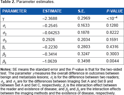
The model in (4) tells that, given V_i, the survival function of Y_ij is

\begin{matrix} \log S (t | v_{i}; x_{i j}, d_{i j}) \\ = \exp {a (t) + y d_{i j} + x_{i j}^{T} θ + d_{i j} x_{i j}^{T} β + v_{i}} . \log S_{0} (t), \end{matrix}

(6)

and it defines the location-scale family mentioned earlier if log S₀(t) = exp(–t). In addition, our model (4) assumes that the intercept is random in S₀(t|v;x), and all other coefficient vectors are fixed, not cluster-specific random. This simplification makes the cluster-specific ROC curve be the same with (2).

Our primary goal of the ROC analysis is the comparison of different diagnostic methods. To do it, we introduce dichotomous covariates x indicating the choice of methods and test their coefficients in model (1). In our motivating example (the example followed in the next section), we have three imaging methods by two readers (two medical doctors who read the images) and we use the three-dimensional covariate vector with two levels (0 or 1), x = (x_r,x_m2,x_m3), where x_r = 1 implies the outcome is recorded by the second reader, x_m2 = 1 implies the outcome is from the second imaging method, and x_m3 = 1 implies the outcome is from the third imaging method.

Finally, the proposed model (1) is a nonlinear mixed-effects model, which is well studied in the literature. Many refined approximations to the likelihood function of the model are proposed and encoded into common statistical packages, including SAS and SPSS. The comparison of different diagnosis methods could be done by testing the regression coefficients of the covariates, indicating the choice of diagnostic methods. This feature is illustrated in details by analyzing a real data in the next section. We refer readers to Davidian and Giltinan¹⁷ for the details of the nonlinear mixed-effects model.

Numerical Study

In this section, we conduct a small numerical study to access the performance of the proposed GS model. The study considers one sample problem to estimate and test the effectiveness of a single diagnostic method with the AUC instead of comparing the ROCs of two or more diagnostic methods. Thus, we have the diagnostic outcomes of two populations, say the normal and cancer populations, by a given diagnostic method.

The data sets for the study are generated as follows. The number of subjects from each population is set as 25 (n = 50 (= 25 + 25)) and 50 (n = 100 (= 50 + 50)). The number of repeated observations per subject is set as m = 2 and m = 4. The ordinal data are generated by categorizing exponentially distributed random variables as follows. For the ith subject of the normal population, we generate m continuous repeatedly measurements from the exponential distribution with the rate λ = 0.1v_i, where log v_i is from normal distribution with mean 0 and variance $σ_{v}^{2}$ . For the subject i in the cancer population, the repeated measurements are from the exponential distribution with the rate λ so that

λ = 0.1 v_{i} \exp (- y),

(7)

where log v_i is again from normal distribution with mean 0 and variance $σ_{v}^{2}$ . The variance $σ_{v}^{2}$ is considered as 1 and 3, where $σ_{v}^{2} = 3$ introduces higher correlation among observations within a subject than $σ_{v}^{2} = 1$ . We transform them to the ordinal data (with five levels indexed by k = 0, 1, 2, 3, 4) using pre-decided grids, which are the five quantiles of the exponential distribution with λ = 0.1.

In (7), γ = 0 implies that there is no difference in the distributions of diagnostic outcomes of normal and cancer populations. In the study, we vary γ = 0, 0.2, 0.4, 0.6, 0.8, 1.0 and consider the powers in testing H₀: γ = 0 (versus γ > 0) as a measure of effectiveness of the procedure. To test the hypothesis, we apply the proposed GS model with link function

\log {- \log (1 - p_{i j} (k | v_{i}; d_{i j}))} = α_{0 k} + d_{i j} y + v_{i},

(8)

where d_i is the indicator variable for the cancer population (it has value 1 if the ith subject is from the cancer population, otherwise, 0) and P_ij(k|v_i;d_ij = P(Y_ij ≤ k|v_i;d_i) for k = 0, 1, 2, 3, 4. The hypothesis is tested by the Z-statistic $Z = \hat{y} / {v a \hat{r} (\hat{y})}^{1 / 2}$ , and both $\hat{y}$ and $va \hat{r} (\hat{y})$ are obtained using the NLMIXED procedure in SAS version 9.3.

For the comparison, we consider the AUC estimate based on the MW statistic, which is popularly used in practice. Here, the MW statistic does not take into account the within-cluster correlation and treats all observations as independent samples. The sample AUC for the ordinal data is computed as the MW statistic with ties as

U = \frac{1}{n_{D} n_{N D}} \sum_{i = 1}^{n_{D}} \sum_{j = i}^{n_{N D}} U_{i j},

(9)

where U_ij = 1, if $Y_{j}^{D} > Y_{j}^{N D}; U_{i j} = 1 / 2,$ if $Y_{j}^{D} = Y_{l}^{N D}$ ; and $U_{i j} = 0, i f Y_{i}^{D} < Y$ Here, n_D is the total number of observations from the disease population and n_ND is that from the normal population. In our case, n_D = n_ND = n · m. The asymptotic variance of the AUC under the assumption of independence of all outcomes is given as follows:

\hat{var} (U) = \frac{n_{D} n_{N D}}{12} {n_{D} + n_{N D} - \frac{\sum_{k = 1}^{5} S_{k} (s_{k}^{2} - 1)}{(n_{D} + n_{N D}) (n_{D} + n_{N D} - 1)}},

(10)

where S_k is the number of observations whose scores are j for k = 1, …, 5. The test for non-effectiveness of the diagnostic method is done using the standardized statistics $Z_{M W} = U / {\hat{var} (U)}^{1 / 2}$ , which follows approximately the standard normal distribution under the null.

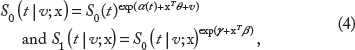
We generate 1000 data sets for each case of $σ_{v}^{2} = 1, 3$ (the variance of random effects) and m = 2, 4 (the number of repetitions with a subject) and evaluate the empirical power by counting the number of rejections among 1000 data sets. The empirical powers of the GS method and MW statistic are plotted in Figure 1. In the figure, “MW (size corrected)” is the empirical size correction of MW test, where 100(1 – α)th empirical percentile of the MW statistic for γ = 0 is used as the critical value, instead of z_α/2, the 100(1 – α/2)th percentile of the standard normal distribution. “MW (size corrected)” is simply added as a reference and is not applicable in practice because we do not have those statistics from the null.

Figure 1.

Power comparison between the proposed grouped-survival model-based and MW-based tests (not considering correlation among outcomes of a single subject). The “size corrected MW” implies the MW test is implemented with an empirically decided critical value. The empirical critical value is decided with the percentile of the (evaluated) MW test statistics for the case γ = 0. (A) $σ_{v}^{2} = 1$ (low within-cluster correlation) and the number of repetitions m = 2. (B) $σ_{v}^{2} = 1$ (low within-cluster correlation) and the number of repetitions m = 4. (C) $σ_{v}^{2} = 3$ (high within-cluster correlation) and the number of repetitions m = 2. (D) $σ_{v}^{2} = 3$ (high within-cluster correlation) and the number of repetitions m = 4.

Figure 1 shows that the size of MW-based test (the power when γ = 0) is biased significantly and its magnitude increases as either $σ_{v}^{2}$ increases or the number of repetition m increases. Both increases of $σ_{v}^{2}$ and m imply the increase in the correlation among repeated observations within a subject (or cluster). On the other hand, the size of the proposed GS model-based test is approximately at the aimed level 0.05, regardless of $σ_{v}^{2}$ and m. The powers of GS-method are comparable to the size-corrected MW test in all cases considered.

Data Example

In this section, we apply our model to the detection of hepatic lesions. The liver is the most frequent site of metastases from various extrahepatic malignancies, and determining the presence of hepatic metastases is important in order to provide the optimal plan for patients who are candidates for surgery and in order to assess prognosis after initial treatment.

The data analyzed in this article are the records of patients who underwent liver MRI with separate acquisition of double contrast enhancement between November 2005 and June 2006. The data are collected from the database of the radiology department at Asan Medical Center in Seoul, Republic of Korea. The data record the test results of the 106 focal liver lesions from 36 patients $(n = 36 a n d \sum_{i = 1}^{n} f_{i} = 106)$ , where f_i denotes the number of the focal hepatic lesions from the ith subject. The 106 focal liver lesions are composed of 51 metastases and 55 benign lesions. Note that the minimum and the maximum of {f₁, …, f₃₆} are 1 and 8, respectively. We take a picture of each lesion with three different methods: MRI with MultiHance (Set A), MRI with Resovist (Set B), and the combination of the original MRI with Resovist and dynamic MRI (Set C). Two readers determine the possibility of malignancy of the detected lesions using a 5-point confidence rating scale (definitely not = 0, probably not = 1, possibly = 2, probably = 3, and definitely = 4). Then, each lesion has six ratings; the combination of two readers (two medical and three imaging methods) and a subject has six x f_i (= n_i) ratings in total. The goal of this experiment is comparing the performance of three picturing methods and two readers. More details on the data including how the data are corrected are available from the study of Hong et al.¹⁴ A summary of the data is presented in Table 1.

Table 1.

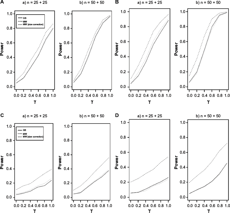
Summary of the data for hepatic metastases.

IMAGING SET	READER	DISEASE	RATINGS
IMAGING SET			Y = 0	Y = 1	Y = 2	Y = 3	Y = 4
A	1	0	46	4	0	5	0
A	1	1	13	1	3	8	26
A	2	0	43	5	2	2	3
A	2	1	6	0	0	3	42
B	1	0	43	3	2	1	6
B	1	1	8	1	1	4	37
B	2	0	44	5	2	2	2
B	2	1	7	2	3	1	38
C	1	0	49	0	1	2	3
C	1	1	2	0	0	8	41
C	2	0	47	3	1	1	3
C	2	1	5	0	1	5	40

Notes: Set A is the MRI with MultiHance, Set B is the MRI with Resovist, and Set C is the combination of the original MRI with Resovist and dynamic MRI (Set C). Reader 0 and Reader 1 are the IDs of radiologists who read the images. Y is the diagnostic results.

Let Y_ij be the jth rating of the ith subject having an ordinal integer mark value between 0 and 4, for i = 1, 2, …, 36 and j = 1, 2, …, n_i; let d_ij be the binary variable, which equals to 1 if the (i, j)th rating is from the disease (positive) group in truth, otherwise 0. For the (i, j)th rating, let x_ij = (x_ijr, x_ij2, x_ij3) be the three-dimensional covariate vector of indicator variables, where x_ijr = 1 if the rating is done by the first reader, x_ij2 = 1 if the rating is on the MRI by Set B, and x_ij3 = 1 if it is by Set C.

We apply the model (1) with the complementary log–log link, so that we have

\begin{matrix} \log {- \log (1 - P_{i j} (k | v_{i}; x_{i j}, d_{i j}))} \\ = α_{0 k} + d_{i j} y + x_{i j}^{T} θ + d_{i j} x_{i j}^{T} β + v_{i}, \end{matrix}

(11)

where $P_{i j} (k | v_{i}; x_{i j}, d_{i j}) = P (Y_{i j} \leq k | v_{i}; x_{i j}, d_{i j}), θ = {(θ_{r}, θ_{2}, θ_{3})}^{T}$ and $β = {(β_{r}, β_{2}, β_{3})}^{T}$ . Let V_J be a random effect from the ith subject and $v_{i -}^{i i d} N (0, σ^{2})$ . Here, γ measures the difference in outcomes between benign and metastasis lesions; v_r, v₂, and v₃ measure the difference between two readers, the difference in imaging methods between Set A and Set B, and the difference between Set A and Set C, respectively; β_r is the interaction effect between the reader and existence of disease; and β₂ and β₃ are the interaction effects between the imaging methods and the existence of disease. Here, the non-zero β implies that the readers and the methods perform differently between the normal and disease groups. In particular, β₂ and β₃ measure the efficacy of the imaging methods.

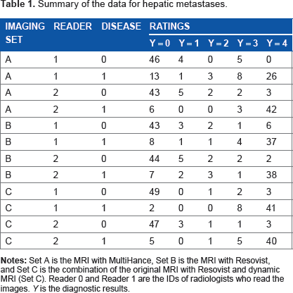
Table 2 displays the parameter estimates calculated from the data, and Figure 1 plots the estimated ROC curves for the six combinations of readers and MRI methods. The results tell that the MRI methods and the reader do not perform differently for normal liver lesions. However, for the tumor lesions, the MRI method Set C performs better than Set A (P-value = 0.0044). In addition, the P-value for jointly testing H₀: β₂ = β₃ = 0 is 0.0160 and that for testing H₀: β₂ – β₃ = 0 is 0.0490. This implies that the MRI method Set C performs better than any of Set A and Set B for tumor lesions. In tumor groups, there is no statistically significant difference between readers.

Table 2.

Parameter estimates.

PARAMETER	ESTIMATE	S.E.	P-VALUE
γ	–2.3688	0.2969	<10⁻⁴
v _r	–0.2545	0.1633	0.1280
v ₂	–0.04253	0.1878	0.8222
v ₃	0.2926	0.2034	0.1591
β_r	–0.2230	0.2803	0.4316
β₂	–0.3414	0.3247	0.3003
β₃	–1.0639	0.3498	0.0044

Notes: SE means the standard error and the P-value is that for the two-sided test. The parameter γmeasures the overall difference in outcomes between benign and metastasis lesions; v_r is for the difference between two readers; v₂, and v₃ are for the differences between Imaging Set A and Set B and between Set A and Set C, respectively; β_r is the interaction effect between the reader and existence of disease; and β₂ and β₃ are the interaction effects between the imaging methods and the existence of disease, respectively.

The covariate-specific ROC curve R(u|x, d) from (11) is in the form of

R (u; x) = u^{\exp (y + x^{T} β)}

(12)

and its AUC is $A (x) = 1 / {1 + \exp (y + x^{T} β)}$ . Figure 1 plots the estimated ROC curves along with their empirical ROC curves. Here, the empirical ROC curves do not take into account the correlation among outcomes within a cluster. For both readers, the curves for Set C are higher than Set A and Set B, indicating that taking pictures of lesion with combination of original MRI with Resovist and dynamic MRI method is superior to use only a single MRI method (Fig. 2).

Figure 2.

Estimated ROC curves of three methods by two readers. The “Empirical” is the empirical ROC curve based on empirical (cumulative) distribution functions of (diagnostic outcomes of) normal and diseased populations. The Empirical disregards the correlations among repeated measurements of a subject and treats them as independent samples. The “Model” is the ROC curve from the model with the estimated parameters.

Table 3 summarizes the estimates of the AUCs for the combinations of a reader and an imaging method. The standard errors (SEs) of the model-based estimates of the AUC are obtained by the delta method. We also report their empirical estimates without taking account the within-cluster correlation of outcomes by Obuchowski.¹¹ The formulas of empirical estimates can also be found from Pepe (Chapter 6.3).¹⁶

Table 3.

The estimates of the AUC and their SEs for the combinations of a reader and a picturing method.

FACTOR	SET A	SET B	SET C
Model
Reader 1	0.914(0.0196)	0.938(0.1226)	0.969(0.0900)
Reader 2	0.930(0.0671)	0.949(0.0967)	0.975(0.1096)
Empirical
Reader 1	0.837(0.0393)	0.849(0.0393)	0.945(0.0393)
Reader 2	0.902(0.0393)	0.892(0.0393)	0.915(0.0393)

Notes: The “Empirical” is estimated using the MW statistic, which disregards the correlation among measurements from a single subject. The SEs of the Empirical are evaluated under the independence assumption of the repeated measurements from a subject, which is rarely true. Thus, they would not be the right numbers. The Model is the estimated AUCs using the formula (13), and its SEs are evaluated using the delta method.

The AUCs may not be always sensible to detect the differences for specific covariates, regardless of whether they are model based or empirical, since they are functional forms of many other components as given:

A (x; y, β_{r}, β_{2}, β_{3}) = 1 / {1 + \exp (y + x^{T} β)}

(13)

On the other hand, the proposed regression model can test the contribution from each covariate separately. To be specific, in our example, if we want to find the performance difference between imaging methods of Set A and Set C for reader 1, the (model-based) AUC estimates are 0.914 and 0.969, respectively. The 95% confidence interval for AUC of Set C is (0.793, 1), which overlaps the confidence interval of AUC for Set A, (0.876, 0.952). This indicates that there is no significant difference between the AUCs of two sets. However, the test based on the proposed regression model makes it possible to test the significance for particular parameter. For example, the P-value of test H₀: β₃ = 0 is 0.0044, and it indicates the existence of significant interaction between sets (A and C) and disease groups (disease and non-disease) at α = 0.05; this implies that the imaging methods A and C perform differently in detecting the cancer.

Conclusion

In this article, we propose a new ROC regression model for clustered ordinal outcomes. The new model views the ordinal outcomes as GS times and uses the grouped-time survival model to define the regression model of the ROC curve. It is shown that the proposed model is closely related with many existing models including the Lehman family and the location-scale family of the ROC curves and further provides their extensions to the random-effects models. Our proposed model has an additional advantage of being easily programmed in many standard statistical packages, which makes it easy to use and interpret. In summary, the model proposed in this article provides a flexible exploratory tool for identifying covariate effects on the ROC curve with clustered ordinal outcomes.

Author Contributions

Conceived and designed the experiments: S-CY, M-SL. Analyzed the data: JK, WS, DHR Wrote the draft of the manuscript: JK, JL. All authors reviewed and approved of the final manuscript.

Footnotes

Appendix

The following SAS code fits the random-effects grouped-time survival model:

DATA Final;

SET Temp; TRT2=0;TRT3=0;RD=0;TD2=0;TD3=0;

IF TRT=2 THEN TRT2=1;

IF TRT=3 THEN TRT3=1;

IF READER=2 AND DISEASE=1 THEN RD=1;

IF TRT=2 AND DISEASE=1 THEN TD2=1;

IF TRT=3 AND DISEASE=1 THEN TD3=1; RUN;

PROC NLMIXED DATA=Final;

PARMS b0=0 b1=0 b2=0 b3=0 b4=0 b5=0 b6=0 b7=0 sd=1 t2=1 t3=2 t4=3 t5=4;

ODS OUTPUT ParameterEstimates=estb;

Z=b0+b1^*DISEASE + b2^*TRT2+b3^*TRT3+b4^*READER+b5^*RD+b6^*TD2+b7^*TD3+u;

DO;

IF (Y=0) THEN p=1-exp(0-exp(t2+z));

ELSE IF (Y=1) THEN p=(1-exp(0-exp(t3+z)))-(1-exp(0-exp(t2+z)));

ELSE IF (Y=2) THEN p=(1-exp(0-exp(t4+z)))-(1-exp(0-exp(t3+z)));

ELSE IF (Y=3) THEN p=(1-exp(0-exp(t5+z)))-(1-exp(0-exp(t4+z)));

ELSE IF (Y=4) THEN p=exp(0-exp(t5+z)); END;

like=LOG(p);

MODEL Y^~ General(like);

Random u^~ NORMAL(0,sd^*sd)

SUBJECT=id;

CONTRAST “all TRT” b6, b7;

ESTIMATE ‘3 vs 2 TRT’ b7-b6;

RUN;

References

Dodd

L.E.

, Pepe

Semi-parametric regression for the area under the receiver operating characteristic curve.

J Am Stat Assoc. 2003; 98: 409–17.

Tosteson

A.A.N.

, Begg

C.B.

A general regression methodology for ROC curve estimation.

Med Decis Making. 1988; 8: 204–15.

Pepe

M.S.

Tree approaches to regression analysis of receiver operating characteristic curves for continuous test results.

Biometrics. 1998; 54: 124–35.

Pepe

M.S.

An interpretation for the ROC curve and inference using GLM procedures.

Biometrics. 2000; 56: 352–9.

Alonzo

T.A.

, Pepe

M.S.

Distribution-free ROC analysis using binary regression techniques.

Biostatistics. 2002; 3: 421–32.

Cai

, Pepe

M.S.

Semi-parametric ROC analysis to evaluate biomarkers for disease.

J Am Stat Assoc. 2002; 97: 1099–107.

Faraggi

Adjusting ROC curves and related indices for covariates.

Statistician. 2003; 52: 179–92.

Schisterman

E.F.

, Faraggi

, Reiser

Adjusting the generalized ROC curve for covariates.

Stat Med. 2004; 23: 3319–31.

Gatsonis

C.A.

Random effects models for diagnostic test accuracy.

Acad Radiol. 1995; 2: S14–21.

10.

Ishwaran

, Gatsonis

A general class of hierarchical ordinal regression models with applications to correlated ROC analysis.

Can J Stat. 2000; 28: 731–50.

11.

Obuchowski

Nonparametric analysis of clustered ROC curve data.

Biometrics. 1997; 53: 170–80.

12.

Lim

, Lee

, Jung

S-H.

A regression model for the AUC of clustered ordinal test results and working independent optimal weights.

Commun Stat Simul Comput. 2012; 41: 1397–410.

13.

Hedeker

, Siddiqui

, Hu

F.B.

Random-effects regression analysis of correlated grouped-time survival data.

Stat Methods Med Res. 2000; 9: 161–79.

14.

Hong

H.S.

, Byun

J.H.

, Won

J.H.

Characterization of liver metastases: the efficacy of biphasic magnetic resonance imaging with ferucarbotran-enhancement.

Clin Radiol. 2010; 65: 701–7.

15.

Gönen

, Heller

Lehmann family of ROC curves.

Med Decis Making. 2010; 30: 509–17.

16.

Pepe

M.S.

The Statistical Evaluation of Medical Tests for Classification and Prediction. London: Oxford University Press; 2004.

17.

Davidian

, Giltinan

D.M.

Nonlinear models for repeated measurement data: an overview and update.

J Agric Biol Environ Stat. 2003; 8: 387–419.

ROC Estimation from Clustered Data with an Application to Liver Cancer Data

Abstract

Keywords

Introduction

Model

Numerical Study

Data Example

Conclusion

Author Contributions

Footnotes

Appendix

References