Sage Journals: Discover world-class research

Abstract

In the frame of the Cox proportional hazard (PH) model, a novel two-step procedure for estimating age-period-cohort (APC) effects on the hazard function of death from cancer was developed. In the first step, the procedure estimates the influence of joint APC effects on the hazard function, using Cox PH regression procedures from a standard software package. In the second step, the coefficients for age at diagnosis, time period and birth cohort effects are estimated. To solve the identifiability problem that arises in estimating these coefficients, an assumption that neighboring birth cohorts almost equally affect the hazard function was utilized. Using an anchoring technique, simple procedures for obtaining estimates of interrelated age at diagnosis, time period and birth cohort effect coefficients were developed.

As a proof-of-concept these procedures were used to analyze survival data, collected in the SEER database, on white men and women diagnosed with LC in 1975–1999 and the age at diagnosis, time period and birth cohort effect coefficients were estimated. The PH assumption was evaluated by a graphical approach using log-log plots. Analysis of trends of these coefficients suggests that the hazard of death from LC for a given time from cancer diagnosis: (i) decreases between 1975 and 1999; (ii) increases with increasing the age at diagnosis; and (iii) depends upon birth cohort effects.

The proposed computing procedure can be used for estimating joint APC effects, as well as interrelated age at diagnosis, time period and birth cohort effects in survival analysis of different types of cancer.

Keywords

cancer survival age time period cohort hazard function lung cancer

Introduction

In cancer epidemiology, survival and hazard functions are valuable characteristics of severity for a given type of cancer. By analyzing temporal trends of these functions, clinicians can evaluate their achievements in cancer diagnosis and treatment. This analysis can also help researchers develop novel approaches and strategies for fighting cancer.

The survival function, S(τ), is the probability for a cancer patient to stay alive longer than a specified time, τ, after cancer diagnosis. This function is related to the hazard function, h(τ), that determines the instantaneous risk (hazard) of death from the cancer at time, τ, given that the patient has survived up to this time:

S (τ) = e^{- H (τ)},

(1)

where $H (τ) = \int_{0}^{τ} h (z) d z$ is the so-called cumulative hazard function.^1,2

For each cancer type, these functions, along with the most common risk factors, such as gender, race, geographical areas of living, etc., also depend on age at diagnosis (ages at which patients were diagnosed with cancer), time period (calendar years when patients were diagnosed with cancer) and birth cohort (calendar years when cancer patients were born) effects.

Traditionally, survival functions have been evaluated from cohort-based follow-up observations by monitoring cancer patient survival in clinical-based registries. To analyze survival data, a single variable Kaplan-Meier method has been widely used.³ The survival functions obtained from these observations adequately describe survival data on cancer cases diagnosed many years ago. Data collected more recently have lower impact on evaluation of survival functions.

To overcome this shortcoming, the period analysis approach and its modification (called period analysis modeling technique) were introduced.^4–8 The latter technique assumes the existence of a linear trend for the conditional survival estimates within the 5–year periods used for modeling. A period of five calendar years was chosen to optimize the most up-to-date and precise estimation of cancer survival function. Compared to traditional cohort-based approaches, the period analysis modeling technique allows one to derive more up-to-date and more precise estimates of survival function for cancer patients. However, the period analysis approach does not consider birth cohort effects.

A multivariate Cox regression approach in the frame of the proportional hazard (PH) model was used to assess the comparative risks or hazard functions of death from cancer.⁹ The PH model assumes that values of the hazard function are proportionally dependent upon the risk factors. A graphical approach using log-log plots was utilized to evaluate the PH assumption. A multivariate Cox regression approach was applied to estimate differences in hazards by histological types of pancreatic cancer. Along with other variables, such as gender, race, histological type, surgery status and cancer stage, age at diagnosis and time period effects were considered, while cohort effects were ignored. As we show below, in the frame of the PH model, age at diagnosis, time period and birth cohort effects are interrelated. To date, there is no numerical method for simultaneous estimation of these interrelated effects.

In this paper we are proposing to extend the Cox PH model and apply it for estimation of the interrelated age-period-cohort effects on cancer survival. It should be noted that this model can be utilized if the parallelism of log-log survival curves is present. In contrast to the single variable Kaplan-Meier approach that accounts only for time to event (survival) data, a multivariate Cox regression approach accounts for many confounding variables, as well as for censored data. In cancer research, the Cox PH model has been widely used for the analysis of data collected in nested case-control, case-cohort, and cohort studies, as well as in clinical trials. However, to our best knowledge, this approach was not used for analysis of data from population-based studies to estimate the interrelated age-period-cohort (APC) effects on cancer survival. The main reason for that is an identifiability problem with multiple estimators that arises in estimating these effects. In this paper we introduce a simple, computationally effective method to solve this identifiability problem. The proposed solution of this problem is analogous to one that we recently utilized for accounting APC effects on cancer incidence rates.^10,11

As a proof-of-concept, the proposed approach was utilized to analyze the SEER data on lung cancer (LC) survival in white men and women. The validity of the PH assumption for analyzing this data was initially checked by assessing the parallelism of log-log survival curves. The proposed approach allowed us to estimate numerically the interrelated age at diagnosis, time period and birth cohort effects on survival and hazard functions of LC in white men and women.

Methodology

Generally, APC analysis refers to a family of statistical techniques for understanding temporal trends of an outcome under consideration (such as cancer incidence or mortality rates, hazard function of death from cancer, etc.). The purpose of this analysis is to determine separate contributions of age, time period of observations, and birth cohort to this outcome.¹² This kind of analysis, along with other data, can also be performed with the use of cancer follow-up survival data collected over a long period of time from large population-based cancer registries (such as, for instance, the Surveillance, Epidemiology, and End Results (SEER) Program).¹³

Statement of the problem

Let us assume that for each patient with a particular type of cancer, there is information on age at diagnosis, date of diagnosis, date of birth, as well as follow-up data on death from the cancer at time, τ, given that the patient has survived up to this time and the right censorship is presented by a dichotomous value (0 or 1). We can group the data by their belonging to the categorical intervals noted by the i, j and l indexes, where index i (i = 1,2, …, n) denotes successive age at diagnosis intervals, index j (j = 1,2, …, m) denotes successive time period intervals, and index l(l = 1,2, …, k) denotes successive birth cohort intervals. Let us denote the corresponding hazard functions for cancer patients with (i,j,l) grouped data by h_i,j,l (τ). This function, along with τ, also depends on the i,j, and l indexes, which are related by the following linear relationship:

l = j - i + n .

(2)

This relationship directly follows from the fact that if an event occurs to an individual of age a in year p then a particular cohort c = p - a must be involved.¹²

To determine the separate contributions of age, period, and cohort effects to the h_i,j,l(τ) function let us use the PH model, which is widely utilized in cancer survival analysis.^1,2 In the frame of this model, the h_i,j,l(τ) function proportionally depends upon age at diagnosis (w_i), time period (v_j) and birth cohort effect coefficients (u_l), as well as on the baseline hazard function (h₀(τ)) the following way:

h_{i j l} (τ) = w_{i} v_{j} u_{l} h_{0} (τ) .

(3)

Now, the APC analysis problem is to estimate the w_i, v_j, and u_l coefficients and the h₀(τ) function, using the patient's survival time data, τ, grouped by the i, j and l indexes. These survival time data also contain information for right censorship presented by dichotomous values (0 or 1). Since the i, j and l indexes are connected by linear relationship (2), values of these coefficients are interrelated and the estimation of these coefficients is an identifiability problem with multiple estimators.¹⁴ It means that there are many solutions to this problem that equally satisfy the observed survival time data and this problem needs to be transferred into the problem that has a single solution. This is the main difficulty in solving this problem. To the best of our knowledge in survival studies, the identifiability problem of APC analysis stated in such a way has not been solved yet.

Computational procedure for solving the problem

Below, we introduce a simple, computationally effective two-step procedure to solve the aforementioned identifiability problem. In the first step, it estimates the influence of joint APC effects on the hazard function, using a Cox PH approach. In the second step, the coefficients for age at diagnosis, time period and birth cohort effects are estimated. To solve the identifiability problem in estimating these coefficients, an additional assumption that neighboring birth cohorts almost equally affect the hazard function is utilized. The proposed procedure uses the same assumption that we have effectively used for accounting APC effects on cancer incidence rates.^10,11 Using an anchoring technique, simple algorithms for obtaining estimates of interrelated age at diagnosis, time period and birth cohort effect coefficients are developed and coded into a computer program. A detailed explanation of this two-step procedure is presented below.

Step 1. Determination of joint age-period-cohort effect coefficients

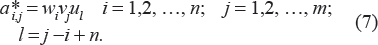
Let us present (3) in the following way:

\begin{array}{l} h_{i, j, l} (τ) = a_{i, j, l} h_{0} (τ) i = 1, 2, \dots, n; \\ j = 1, 2, \dots, m; l = j - i + n; \end{array}

(4)

where a_i,j,l designates the product of w_iv_ju_l and h₀(τ). Since l = j - i + n, grouping by three indexes i, j, and l can be reduced to the grouping by two indexes, i and j, and the system (4) can be presented as:

h_{i, j} (τ) = a_{i, j} h_{0} (τ) i = 1, 2, \dots, n; j = 1, 2, \dots, m;

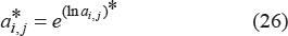
Now, using system (5) with observed survival data, one can assess each a_i,j and its standard error (SE), as well as h₀(τ). For this purpose, the Cox PH regression approach that uses maximum likelihood estimates can be utilized. The $a^{*}_{i, j}$ estimates (here and below the asterisks designate the estimates) need to be anchored to one of the coefficients to be estimated. This coefficient, say, $a^{*}_{i_{0}, j_{0}},$ is assumed to be equal to 1 and its SE is assumed to be equal to 0, (i.e. $a^{*}_{i_{0}, j_{0}} = 1$ and SE $(a^{*}_{i_{0}, j_{0}} = 0),$ where i₀ and j₀ are indexes of the anchored coefficient a_i,j).

Note: The Cox PH model, that is a particular case of the PH model, is usually written in terms of an exponential expression:

h_{i, j} (τ) = h_{0} (τ) e^{\ln a_{i, j}},

(6)

where parameters to be estimated are lna_i,j. This exponential form of the expression (6) provides non-negative estimates of a_i,j.¹

Step 2. Determination of coefficients for interrelated age at diagnosis, time period and birth cohort effects

The estimates $a *_{i, j},$ obtained on the previous step, can be used for estimating the w_i, v_j, and u_l, coefficients. For this purpose, three sets of estimates can be obtained from the system of i × j conditional equations

a *_{i, j} = w_{i} v_{j} u_{l} i = 1, 2, \dots, n; j = 1, 2, \dots, m; l = j - i + n .

(7)

These sets are: (i) estimates for the age at diagnosis coefficients $(w_{i}^{*})$ ; (ii) estimates for the time period coefficients $(v_{j}^{*})$ ; and (iii) estimates for the birth cohort effect coefficients $(u_{l}^{*})$ . However, due to the linear relationship (2) between indexes i, j and l, these three effects are interrelated. As a result, the identifiability problem with multiple estimators arises in system (7): different combinations of corresponding effect coefficients equally satisfy the observations of cancer survival. This problem is analogous to the problem of accounting for effects of age, period, and cohort on cancer incidence rates.^12,15–18

To solve the identifiability problem in APC analysis it is necessary to make additional assumptions.^12,15–18 For such an assumption, we hypothesize that the neighboring birth cohorts almost equally affect the cancer survival data. The rationale for this assumption is that, in practice, the adjacent cohorts are overlapping in time intervals and thus the values of the corresponding cohort effects should be close.¹⁴ Based on this assumption, we proposed a novel computing procedure for numerical estimation of interrelated age at diagnosis, time period and birth cohort coefficients on cancer survival and hazard functions.

Estimation of age at diagnosis effect coefficients

Let us consider the i × j matrix with $a_{i, j}^{*}$ elements presented in system (7). By dividing the corresponding elements of the neighboring rows (with indexes i and i + 1 or i + 1 and i) of this matrix, one can obtain two systems of equations (v_j coefficients are canceled out):

\begin{array}{l} \frac{a_{i, j}^{*}}{a_{i + 1, j}^{*}} = \frac{w_{i}}{w_{i + 1}} \frac{u_{l}}{u_{l - 1}}; i = 1, \dots, n - 1; \\ j = 1, \dots, m; l = j - i + n \end{array}

(8)

and

\begin{array}{l} \frac{a_{i, j}^{*}}{a_{i + 1, j}^{*}} = \frac{w_{i}}{w_{i + 1}} \frac{u_{l}}{u_{l - 1}}; i = 1, \dots, n - 1; \\ j = 1, \dots, m; l = j - i + n \end{array}

(9)

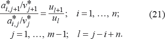
Note: (8) provides (n - 1) × m conditional equations for assessing n - 1 ratios of time period coefficients $(w_{i}^{/} w_{i + 1}, i = 1, \dots, n - 1)$ , and m – 1 + n - 1 ratios of the cohort effect coefficients $(u_{l}^{/} u_{l - 1}, l = 2, \dots, m - 1 + n)$ . Analogously, (9) provides (n - 1) × m conditional equations for assessing n – 1 ratios of time period coefficients $(w_{i + 1}^{/} w_{i,} i = 1, \dots, n - 1)$ , and m – 1 + n – 1 ratios of cohort effect coefficients $(u_{l - 1}^{/} u_{l}, 1 = 2, \dots, m - 1 + n)$ .

Assuming that any pair of the neighboring cohorts has a cohort effect coefficient ratio close to 1, the following pair of systems can be obtained:

\frac{a_{i, j}^{*}}{a_{i + 1, j}^{*}} = \frac{w_{i}}{w_{i + 1}}; i = 1, \dots, n - 1; j = 1, \dots m

(10)

and

\frac{a_{i, j}^{*}}{a_{i + 1, j}^{*}} = \frac{w_{i}}{w_{i + 1}}; i = 1, \dots, n - 1; j = 1, \dots, m

(11)

When coefficients of variation of estimates $a_{i, j}^{*}$ are small, SEs of the ratios $a_{i, j}^{*} / a_{i, j + 1}^{*}$ and $a_{i, j + 1}^{*} / a_{i, j}^{*}$ can be calculated by standard rules of error propagation.¹⁹ For estimation of $w_{i} / w_{i + 1}$ and $w_{i + 1} / w_{i},$ a least squares method can be applied and the most efficient estimates for these ratios are the weighted means of the values a_i,j^*/a_i,j+1^* and a_i,j+1^*/a_i,j^* averaged through index j, correspondingly (weights are given as reciprocals of the square of their standard errors). The SEs of the estimates ${(w_{i} / w_{i + 1})}^{*}$ ^* and ${(w_{i + 1} / w_{i})}^{*}$ ^* can be calculated in a standard way. In fact, after anchoring the age at diagnosis coefficient at index i₀, assuming $w_{i}_{_{0}} = 1$ and SE $(w_{i}_{_{0}} = 0)$ , one can obtain the following recurrent estimates of $w_{i}^{*}$ :

\begin{array}{l} w_{i_{0} + 1}^{*} = {(\frac{w_{i_{0} + 1}}{w_{i_{0}}})}^{*}, w_{i_{0} + 2}^{*} = {(\frac{w_{i_{0} + 2}}{w_{i_{0} + 1}})}^{*} w_{i_{0} + 1}^{*}, \dots, \\ w_{n}^{*} (\frac{w_{n}}{w_{n - 1}})^{^{^{^{*}}}} w_{n - 1}^{*} \end{array}

(12)

and

\begin{array}{l} w_{i_{0} - 1}^{*} = {(\frac{w_{i_{0} - 1}}{w_{i_{0}}})}^{*}, w_{i_{0} - 2}^{*} = {(\frac{w_{i_{0} - 2}}{w_{i_{0} - 1}})}^{*} w_{i_{0} - 1}^{*}, \dots, \\ w_{1}^{*} (\frac{w_{1}}{w_{2}})^{*} w_{2}^{*} . \end{array}

(13)

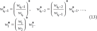
Note 1: Index i₀ is defined from the corresponding index of the anchored coefficient $a_{i_{0}, j_{0}}^{*} = 1.$ The SE of $w_{i}^{*}$ can be calculated by the standard rules of error propagation by means of the estimates ${(w_{_{i}} / w_{i + 1})}^{*}$ , ${(w_{i + 1} / w_{_{i}})}^{*}$ and their SEs.

Note 2: Analogous to our previous works for the APC analysis of cancer incidence rates,^10,11 one can show that errors of the estimates $w_{i}^{*}$ (as well as errors of $v_{j}^{*}$ and $u_{l}^{*}$ ) are distributed approximately normally. This was used to test the null hypotheses ( $w_{i} = w_{i_{0}}, v_{j} = v_{j_{_{0}}}$ , and $u_{l} = u_{l_{0}}$ ) by the standard z-test.

Estimation of time period effect coefficients

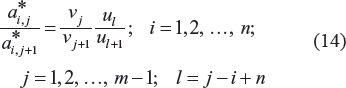
By dividing the corresponding elements of the neighboring columns (with indexes j and j + 1 or j + 1 and j) of the i × j matrix with $a_{i, j}^{*}$ elements, one can obtain the following two systems of equations (w_i coefficients are canceled out):>

\begin{array}{l} \frac{a_{i, j}^{*}}{a_{i, j + 1}^{*}} = \frac{v_{j}}{v_{j}_{+ 1}} \frac{u_{l}}{u_{l}_{+ 1}}; i = 1, 2, \dots, n; \\ j = 1, 2 \dots, m - 1; l = j - i + n \end{array}

(14)

and

\begin{array}{l} \frac{a_{i, j + 1}^{*}}{a_{i, j}^{*}} = \frac{v_{j}_{+ 1}}{v_{j}} \frac{u_{l}_{+ 1}}{u_{l}}; i = 1, 2, \dots, n; \\ j = 1, 2 \dots, m - 1; l = j - i + n . \end{array}

(15)

Note: (14) provides n × (m – 1) conditional equations for assessing m – 1 ratios of time period coefficients $(v_{j} / v_{j + 1}, j = 1, \dots, m - 1),$ and m – 1 + n – 1 ratios of cohort effect coefficients $(u_{l} / u_{l + 1}, l = 1, \dots, m - 1 + n - 1) .$ Analogously, (15) provides n × (m – 1) conditional equations for assessing m – 1 ratios of time period coefficients $(v_{j + 1} / v_{j}, j = 1, \dots, m - 1),$ and m – 1 + n – 1 ratios of cohort effect coefficients $(u_{l + 1} / u_{l}, l = 1, \dots, m - 1 + n - 1) .$ Assuming that for any pair of the neighboring cohorts, the ratio of their cohort effect coefficients is close to 1, one can obtain from (14) and (15) a pair of systems:

\frac{a_{i, j}^{*}}{a_{i, j + 1}^{*}} = \frac{v_{j}}{v_{j + 1}}; i = 1, 2, \dots, n; j = 1, 2, \dots, m - 1

(16)

and

\frac{a_{i, j + 1}^{*}}{a_{i, j}^{*}} = \frac{v_{j + 1}}{v_{j}}; i = 1, 2, \dots, n; j = 1, 2, \dots, m - 1.

(17)

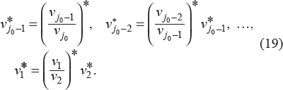
When coefficients of variation of estimates $a_{i, j}^{*}$ are small, SEs of the ratios $a_{i, j}^{*} / a_{i, j + 1}^{*}$ and $a_{i, j + 1}^{*} / a_{i, j}^{*}$ can be calculated by standard rules of error propagation.¹⁹ For estimation of $v_{j} / v_{j + 1}$ and $v_{j + 1} / v_{j}$ a least squares method can be applied and the most efficient estimates for these ratios are the weighted means of the values $a_{i, j}^{*} / a_{i, j + 1}^{*}$ and $a_{i, j + 1}^{*} / a_{i, j}^{*}$ averaged through index i, correspondingly (weights are given as reciprocals of the square of their standard errors). The SEs of the estimates ${(v_{j} / v_{j + 1})}^{*}$ and ${(v_{j + 1} / v_{j})}^{*}$ can be calculated in a standard way.

After anchoring the age at diagnosis coefficient at index j₀, assuming $v_{j_{0}} = 1$ and $S E (v_{j_{0}}) = 0,$ one can obtain the following recurrent estimates of $v_{j}^{*}$ :

\begin{array}{l} v_{j_{0} + 1}^{*} = {(\frac{v_{j_{0} + 1}}{v_{j_{0}}})}^{*}, v_{j_{0} + 2}^{*} = {(\frac{v_{j_{0} + 2}}{v_{j_{0} + 1}})}^{*} v_{j_{0} + 1}^{*}, \dots, \\ v_{m}^{*} = {(\frac{v_{m}}{v_{m - 1}})}^{*} v_{m - 1}^{*} \end{array}

(18)

and

\begin{array}{l} v_{j_{0} - 1}^{*} = {(\frac{v_{j_{0} - 1}}{v_{j_{0}}})}^{*}, v_{j_{0} - 2}^{*} = {(\frac{v_{j_{0} - 2}}{v_{j_{0} - 1}})}^{*} v_{j_{0} - 1}^{*}, \dots, \\ v_{1}^{*} = {(\frac{v_{1}}{v_{2}})}^{*} v_{2.}^{*} \end{array}

(19)

The SE of $v_{j}^{*}$ can be calculated by the standard rules of error propagation by means of the estimates ${(v_{j} / v_{j + 1})}^{*}$ and ${(v_{j + 1} / v_{j})}^{*}$ and their SEs.

Note 1: Index j₀ is defined by the anchored coefficient $a_{i_{0}, j_{0} = 1.}^{*}$

Note 2: The preceding method for estimation of time period effect coefficients is similar to the method for estimation of age at diagnosis effect coefficients. In the first case, the conditional equations are derived dividing the corresponding elements of the neighboring rows of i × j matrix with $a_{i, j}^{*}$ . In the second case, the conditional equations are derived dividing the corresponding elements of the neighboring columns.

Estimation of birth cohort effect coefficients

One way to assess u_l is as follows. After evaluating the time period effect coefficients, $v_{j}^{*}$ , one can correct the $a_{i, j} *$ coefficients for time period effects by dividing them by $v_{j}^{*}$ . From (7) and (14), the following two systems of conditional equations can be derived:

\begin{array}{l} \frac{a_{i, j}^{*} / v_{j}^{*}}{a_{i, j + 1}^{*} / v_{j + 1}^{*}} = \frac{u_{l}}{u_{l + 1}}; i = 1, \dots n; \\ j = 1, \dots, m - 1; l = j - 1 + n \end{array}

(20)

and

\begin{array}{l} \frac{a_{i, j + 1}^{*} / v_{j + 1}^{*}}{a_{i, j}^{*} / v_{j}^{*}} = \frac{u_{l + 1}}{u_{l}}; i = 1, \dots n; \\ j = 1, \dots, m - 1; l = j - 1 + n . \end{array}

(21)

By the standard rules of error propagation, one can obtain SEs of the ratios of the corrected coefficients $a_{i, j}^{*} / v_{j}^{*}$ and $a_{i, j + 1}^{*} / v_{j + 1}^{*}$ by means of the standard errors of $a_{i, j}^{*}, v_{j,}^{*} a_{i, j + 1}^{*}$ and $v_{j + 1}^{*}$ . Similar to the ratios of the time period coefficients, the ratios $u_{l} / u_{l + 1}$ and $u_{l + 1} / u_{l}$ can be estimated by the weighted means of values of the left sides of systems (20) and (21). Weights should be given according to the SEs of the corrected coefficients (reciprocal of squares of the SEs). The index of the cohort coefficient to be anchored can be simply obtained from the relationship (2) between the j, l, and i indexes.

By setting $u_{l_{0}} = 1$ and $(S E (u_{l_{0}}) = 0)$ , all cohort coefficients and their SEs can be estimated by a procedure analogous to one used for determination of time period coefficients:

\begin{array}{l} u_{l_{0} + 1}^{*} = {(\frac{u_{l_{0} + 1}}{u_{l_{0}}})}^{*}, u_{l_{0} + 2}^{*} = {(\frac{u_{l_{0} + 2}}{u_{l_{0} + 1}})}^{*} u_{l_{0} + 1}^{*}, \dots, \\ u_{k}^{*} = {(\frac{u_{k}}{u_{k - 1}})}^{*} u_{_{k - 1}}^{*}; k = m - 1 + n \end{array}

(22)

and

\begin{array}{l} u_{l_{0} - 1}^{*} = {(\frac{u_{l_{0} - 1}}{u_{l_{0}}})}^{*}, u_{l_{0} - 2}^{*} = {(\frac{u_{l_{0} - 2}}{u_{l_{0} - 1}})}^{*} u_{l_{0} - 1}^{*}, \dots, \\ u_{1}^{*} = {(\frac{u_{1}}{u_{2}})}^{*} u_{2}^{*} . \end{array}

(23)

Note: Index l₀, for anchoring the birth cohort coefficient is simply derived as: l₀ = j₀ – i₀ + n. The SE of $u_{l}^{*}$ can be calculated by the standard rules of error propagation by means of the estimates ${(u_{l} / u_{l + 1})}^{*}$ and ${(u_{l + 1} / u_{l})}^{*}$ , and their SEs.

Additional details of the proposed procedure are discussed below on the example of analysis of lung cancer (LC) survival data collected in the SEER database.

Potential limitations

The proposed extension of the Cox PH model has several potential limitations. First, this model can be utilized only if the parallelism of log-log survival curves is present. However, the problem of visual evaluation of the parallelism by graphical approaches is to decide “how parallel is parallel?” For a given data set, this decision can be quite subjective. Therefore, we utilized the recommendation of a conservative strategy proposed by Kleinbaum and Klein¹ suggesting that the PH assumption is satisfied if there is not strong evidence for the non-parallelism of considered log-log survival curves.

Second, to solve the identifiability problem, the proposed approach uses an assumption that neighboring birth cohorts almost equally affect the cancer survival data. Therefore, after estimating the birth cohort coefficients and their SEs, the validity of this assumption needs to be verified. If the obtained estimates of some neighboring birth cohort coefficients are statistically different (i.e. validity of this assumption will not be proved by obtained results of calculations), the results cannot be fully justifiable.

It could also be argued that the requirement for categorizing the age at diagnosis, time-period, and birth cohort by equally-sized time intervals reduces areas of possible application of the proposed procedure. By admitting this limitation, we suggest that in practice, the quantitative estimation of the age at diagnosis, time period and birth cohort effect coefficients mainly depends on the amount and quality of the collected data rather than on the use of the equally-sized time intervals. Indeed, according to common practice used in cancer epidemiology, to smooth out random fluctuations in cancer incidence rates, the age at diagnosis, time period and birth cohort intervals are grouped in 5-year time intervals.¹⁸ When the amount of analyzed data is large enough, these time intervals can be diminished to, say, 3 or 4 years that will result in improved accuracy of coefficients determination. However, when the collected data is relatively small, the length of these intervals can be enlarged up to 10 years.¹² The price of this, however, will be the lower accuracy in calculated coefficients.

In principle, the approach proposed in this work can be further extended for cases when the age at diagnosis and time period intervals have different durations. For this purpose, the technique proposed in the literature²⁰ can be utilized. However, it poses additional identifiability problems²⁴ and the use of this technique requires the development of a more complicated computational procedure, while benefits of its use are questionable. Therefore, we decided to keep such an extension out of the scope of this work.

Example

Estimation of APC effects in lung cancer survival analysis

The proposed procedure was used for estimation of the APC effects in LC survival of white men and women. Selections of LC cases and data preparation, as well as implementation of the proposed procedure and analysis of the obtained results, are presented below.

Selection of LC cases and data preparation

In this work, we used the SEER database that contains cancer follow-up survival data collected 1973 through 2004 in the SEER 9 Registries¹³ (Connecticut, Detroit, Hawaii, Iowa, New Mexico, San Francisco-Oakland, Utah, Atlanta (1975–2004), and Seattle-Puget Sound (1975–2004)). From this database, we selected cases for white men and white women aged 40–84 and diagnosed with LC in the 1975–1999 time period, for a total of 272,604 cases. By using the same data processing methodology as described in the SEER Survival Monograph²¹ and our previous study,²² we excluded 38,463 cases that were not first primary cancers; from the obtained subset, we excluded 5,006 cases that were diagnosed via death certificate or at autopsy only; then, we excluded 16,413 cases that were not microscopically confirmed by a pathologist, yielding a total of 212,722 cases (134,360 male and 78,362 female). Choosing the 1975–1999 time period allowed us to analyze the survival with a minimum of five years of follow-up data for LC patients diagnosed in 1999 or earlier. For the selected cases, the survival time was measured in months from the date of diagnosis until the date of death. Cases lost to follow-up were right-censored at the time of the last known follow-up, and patients alive at the end of our study period (December 31, 1999) were right-censored at this date.

The ages of LC patients at the time of diagnosis were divided in nine age at diagnosis intervals, denoted by index i:. i = 1 for 40–44; i = 2 for 45–49; …; i = 8 for 75–79; and i = 9 for 80–84. To get a sufficiently large sample size for statistical analysis, data for the age groups 40 years and over was used (in this case, the number of patients within each age at the diagnosis group exceeds 300). The considered 25-year range of observations (1975–1999) of LC patients was divided into five 5-year time period intervals denoted by index j: j = 1 for 1975–1979; j = 2 for 1980–1984; j = 3 for 1985–1989; j = 4 for 1990–1995; and j = 5 for 1995–1999. In addition, 13 birth cohorts corresponding to the aforementioned age at diagnosis and time periods were divided into 5-year intervals denoted by index l (l = j - i + 9): (l = 1) 1895–99; (l = 2) 1900–04; …; (l = 12) 1950–54; and (l = 13) 1955–59.

For the PH model, the hazard function of LC was presented as h_i,j,l(τ)=w_i,v_j,u_l,h_o(τ) which is a function of the age at diagnosis (w_i), time period (v_j) and birth cohort (u_l) coefficients, as well as the baseline hazard function, h₀(τ). For further convenience, we present this model in Table 1. In this table, hazard functions h_i,j,l(τ)=w_i,v_j,u_l,h_o(τ) are located in the following way: for a given age at diagnosis interval (i) along the row; for a given time period interval (j) along the column; and for a given birth cohort interval (l) along the diagonal. From this table, it is clear that indexes i, j and l are interrelated: any combination of two indexes simply defines the third index (for instance, the row and column defines the diagonal, etc.).

Validation of the PH model

To test the validity of the PH model given by formulas (1) and (2), we used a graphical approach using log-log plots.¹ According to this approach, for each (I,j) cell of Table 1 we plotted the survival curves, S^*, as a function of time τ determined by the method of Kaplan-Meier and then considered the ln(–ln S^*) curve.¹ The parallelism of the log-log survival plots for different cells (i,j) provides one with a graphical approach for assessing the PH assumption. In fact, from (1) and (3) it follows:

- \ln S (τ, w_{i,} v_{j,} u_{l}) = w_{i,} v_{j,} u_{l} \int_{0}^{τ} h_{0} (z) d z

(24)

and

\ln (- \ln S (τ, w_{i,} v_{j,} u_{l}) = \ln (w_{i,} v_{j,} u_{l}) + \ln [\int_{0}^{τ} h_{0} (z) d z] .

(25)

Table 1

Presentation of the hazard function h(τ, w_i, v_j, u_l) by age at diagnosis (w_i), time period (v_j) and birth cohort (u_l) effect coefficients, and the baseline hazard function, h₀(τ).

Notes: The abbreviation, “mp, t_i,” indicates the midpoint of the i-th age at diagnosis interval. Arrows show directions (along diagonals) of changing hazard functions of death from cancer for patients born in the given intervals of calendar years (birth cohort intervals).

When the PH assumption is valid, it follows from formulas (24) and (25) that ln(–ln S(τ,v_j,u_l,w_i) will represent the logarithm of the cumulative baseline hazard function of death from cancer, H_o(τ)=ln[ʃ_o^τh₀(z)dz], shifted along the ordinate axis by the value of ln(w_iv_ju_l). After inspecting the log-log survival plots for each cell of Table 1, we accepted the PH models for LC for both men and women (data not shown).

Results and Discussion

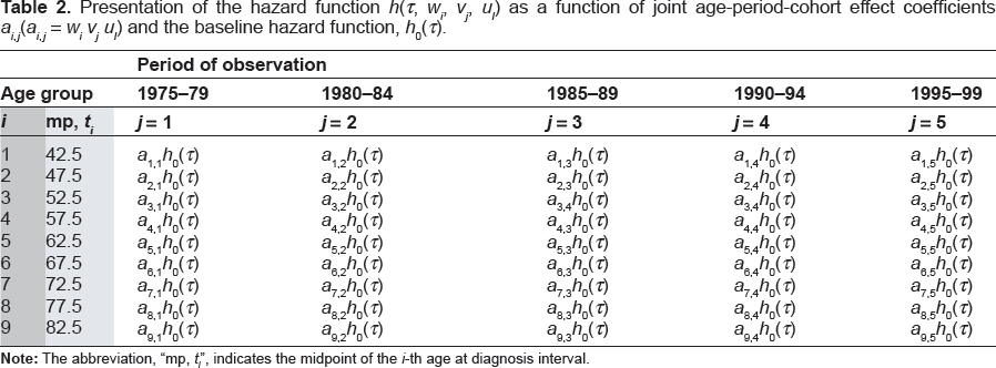
To estimate the joint APC effects in the frame of the Cox PH model, we used Table 2, where for each cell a_i,j = w_iv_ju_l (see the section Step 1, above).

Table 2

Presentation of the hazard function h(τ, w_i, v_j, u_l) as a function of joint age-period-cohort effect coefficients a_i,j(a_i,j = w_i v_j u_l) and the baseline hazard function, h₀(τ).

Period of observation
Age group		1975–79	1980–84	1985–89	1990–94	1995–99
i	mp, t_i	j = 1	j = 2	j = 3	j = 4	j = 5
1	42.5	a_{1, 1}h₀(τ)	a_{1, 2}h₀(τ)	a_{1, 3}h₀(τ)	a_{1, 4}h₀(τ)	a_{1, 5}h₀(τ)
2	47.5	a_{2, 1}h₀(τ)	a_{2, 2}h₀(τ)	a_{2, 3}h₀(τ)	a_{2, 4}h₀(τ)	a_{2, 5}h₀(τ)
3	52.5	a_{3, 1}h₀(τ)	a_{3, 2}h₀(τ)	a_{3, 4}h₀(τ)	a_{3, 4}h₀(τ)	a_{3, 5}h₀(τ)
4	57.5	a_{4, 1}h₀(τ)	a_{4, 2}h₀(τ)	a_{4, 3}h₀(τ)	a_{4, 4}h₀(τ)	a_{4, 5}h₀(τ)
5	62.5	a_{5, 1}h₀(τ)	a_{5, 2}h₀(τ)	a_{5, 3}h₀(τ)	a_{5, 4}h₀(τ)	a_{5, 5}h₀(τ)
6	67.5	a_{6, 1}h₀(τ)	a_{6, 2}h₀(τ)	a_{6, 3}h₀(τ)	a_{6, 4}h₀(τ)	a_{6, 5}h₀(τ)
7	72.5	a_{7, 1}h₀(τ)	a_{7, 2}h₀(τ)	a_{7, 3}h₀(τ)	a_{7, 4}h₀(τ)	a_{7, 5}h₀(τ)
8	77.5	a_{8, 1}h₀(τ)	a_{8, 2}h₀(τ)	a_{8, 3}h₀(τ)	a_{8, 4}h₀(τ)	a_{8, 5}h₀(τ)
9	82.5	a_{9, 1}h₀(τ)	a_{9, 2}h₀(τ)	a_{9, 3}h₀(τ)	a_{9, 4}h₀(τ)	a_{9, 5}h₀(τ)

Note: The abbreviation, “mp, t_i”, indicates the midpoint of the i-th age at diagnosis interval.

To estimate the a_i,j coefficients, we used the Cox PH model, written in terms of an exponential expression (6), and utilized the MATLAB function, “coxphfit”. (It should be noted that for this purpose, other programs for Cox PH regression analysis can also be used.) For each (i,j) cell (where i = 1,2, …, 9; j = 1,2, …, 5) two files were used as input for this function. The first file contained the survival time data, $τ_{i, j, ρ} = τ_{i, j, l, ρ},$ where l = j - i + 9, and ρ denotes the patient's identification index. The second file contained dichotomous values (0 or 1) for the censorship status of each patient. As output data, the coxphfit function provided the estimates (ln a_i,j)^* and SE[(ln a_i,j)^*], and the estimates of the cumulative baseline $H_{0}^{*} (τ)$ for $τ = τ_{i, j, ρ}$ .

We obtained the estimates $a_{i, j}^{*}$ and $S E (a_{i, j}^{*})$ by the formulas:

a_{i, j}^{*} = e^{{(\ln a_{i, j})}^{*}}

(26)

and

S E (a_{i, j}^{*}) = a_{i, j}^{*} S E [{(\ln a_{i, j})}^{*}] .

(27)

To obtain estimates of the age at diagnosis, time period and birth cohort effect coefficients ( $w_{i}^{*}, v_{j}^{*}$ and $u_{l}^{*}$ , correspondingly), we used our newly developed MATLAB computing program, called the “apcsur” function. This program implements algorithms described above (see the section Step 2) and uses the estimates $a_{i, j}^{*}$ and $(a_{i, j}^{*})$ , as well as indexes of the age at diagnosis, time period and birth cohort intervals to be anchored as input data. The coefficients for the anchored intervals were taken equal to 1 and their SE equal to 0. Values of other coefficients were estimated relative to the values of the anchored coefficients. The estimates of the $w_{i}^{*}, v_{i}^{*}$ and $u_{l}^{*}$ coefficients were obtained as output data of the “apcsur” function.

In this work, the age at diagnosis, time period, and birth cohort effect coefficients with median indexes of i = 5, j = 3 and l = 7 were chosen as anchors; values of these coefficients were taken as w₅ = 1, v₃ = 1 and u₇ = 1 and their SEs were taken equal to 0. The anchored coefficients were chosen based on our numerical experiments and showed (data not presented) that, in this case, the SEs of the majority of coefficients to be estimated were smaller than for any other combination.

Table 3 presents the estimates of the age at diagnosis effect coefficients, $w_{i}^{*}$ , and their SEs for white men and women with LC. Statistical differences between these coefficients and the coefficient for the anchored age interval, 60–64, with a value set to be equal to 1, were measured by P-values calculated using the standard z-test. The obtained P-values are shown in Table 3; P-values for the coefficients statistically distinguishable from 1 (with the significance level of 0.05) are shown in italics. Figure 1 shows the trends of the age at diagnosis effect coefficients in white men (A) and women (B). As can be seen, for both men and women, the estimates of age at diagnosis coefficients increase with age, i.e. the hazard of death from LC increases with age. Because, for a given τ, from formula (1) it follows that when the hazard function is increasing, the survival function is decreasing, we can conclude that LC survival rates decrease with age. This statement is consistent with the conclusion made in this work,²³ which is that the cancer survival rates decrease with age.

Table 3.

Estimated values of the age at diagnosis coefficients w_i^*, their standard errors (SE), and P-values characterizing the statistical difference between the estimated coefficient and the anchored coefficient.

Age interval index	White men		White women
Age interval index	$w_{i}^{*} \pm S E$	P-value	$w_{i}^{*} \pm S E$	P-value
1	0.77 ± 0.03	<0.0001	0.78 ± 0.04	<0.0001
2	0.85 ± 0.02	<0.0001	0.84 ± 0.03	<0.0001
3	0.88 ± 0.02	<0.0001	0.86 ± 0.02	<0.0001
4	0.95 ± 0.01	<0.0001	0.94 ± 0.02	<0.0001
5	1.00		1.00
6	1.08 ± 0.02	<0.0001	1.06 ± 0.02	<0.0001
7	1.20 ± 0.02	<0.0001	1.19 ± 0.02	<0.0001
8	1.34 ± 0.03	<0.0001	1.36 ± 0.04	<0.0001
9	1.33 ± 0.04	<0.0001	1.37 ± 0.05	<0.0001

Notes: The coefficient for age interval 5 is the anchored coefficient and is defined as 1.0. Italicized P-values denote coefficients statistically distinguishable from 1.0 (with significance level 0.05).

Figure 1

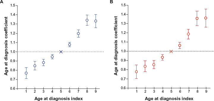
Variation of age at diagnosis coefficients, anchored at index 5, with time period index (i), in white men (A) and white women (B).

Table 4 presents for white men and women with LC estimates of the time period effect coefficients $v_{j}^{*}$ and their SEs, as well as P-values calculated using the standard z-test, for four time period effect coefficients compared to 1 (that is the anchored coefficient for the 1985–89 time period). Figure 2 shows that trends of these coefficients in white men (A) and women (B) demonstrate a slight decrease with time, i.e. the hazard of death from LC has somewhat decreased since the 1975–1999 time period. (More detailed analysis of improvement in LC survival over time is given below, see Table 6). This conclusion is different from the conclusion made by Bassily et al.²³ that states that the LC survival has not improved over three decades. One possible explanation of this discrepancy is the use of different approaches in analysis of the observed survival data: in this work²³ a single variable Kaplan-Meier approach that accounts only time to event (survival) data was used, while in our work we used a modified multivariate Cox regression approach that additionally accounts for interrelated APC effects on cancer survival.

Table 4

Estimated values of the time period coefficients $v_{j}^{*}$ , their standard errors (SE), and P-values characterizing the statistical difference between the estimated coefficient and the anchored coefficient.

Time period index	White men		White women
Time period index	$v_{j}^{*} \pm S E$	P-value	$v_{j}^{*} \pm S E$	P-value
1	1.06 ± 0.02	0.0003	1.04 ± 0.02	0.06
2	1.00 ± 0.01	0.62	1.02 ± 0.02	0.18
3	1.00		1.00
4	0.92 ± 0.01	<0.0001	0.95 ± 0.01	0.0003
5	0.91 ± 0.01	<0.0001	0.93 ± 0.02	<0.0001

Notes: The coefficient for time period index 3 is the anchored coefficient and is defined as 1.0. Italicized P-values denote coefficients statistically distinguishable from 1.0 (with significance level 0.05).

Figure 2

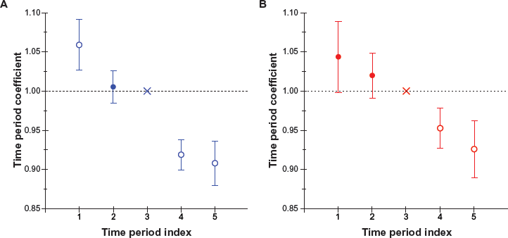
Variation of time period coefficients, anchored at index 3, with time period index (j), in white men (A) and white women (B).

Table 5 presents for white men and women with LC estimates of the birth cohort effect coefficients, $u_{l}^{*}$ , and their SEs, as well as P-values calculated using the standard z-test for twelve birth cohort effect coefficients compared to 1 (that is the anchored coefficient for the 1925–29 birth cohort). Figure 3 presents trends of these coefficients in white men (A) and women (B). As can be seen, for men three (from eight) birth cohort effect coefficients (namely, the coefficients for the 1895–99, 1945–49, and 1950–54 birth cohort periods) are statistically distinguishable from the coefficient of the anchored cohort, 1925–29. For women, only one birth cohort effect coefficient for 1895–99 is statistically distinguishable from the coefficient 1 of the anchored cohort, 1925–29. These data suggest that influence of the birth cohort effects on the hazard of death from LC should not be ignored in the LC survival analysis.

Figure 3

Variation of birth cohort coefficients, anchored at index 7, with birth cohort index (l), in white men (A) and white women (B).

Table 5

Estimated values of the birth cohort coefficients, $u_{l}^{*}$ , their standard errors (SE), and P-values characterizing the statistical difference between the estimated coefficient and the anchored coefficient.

Birth cohort index	White men		White women
Birth cohort index	$u_{l}^{*} \pm S E$	P-value	$u_{l}^{*} \pm S E$	P-value
1	1.20 ± 0.08	0.006	1.25 ± 0.12	0.04
2	0.94 ± 0.04	0.15	0.97 ± 0.06	0.56
3	1.04 ± 0.03	0.23	0.98 ± 0.04	0.72
4	0.99 ± 0.02	0.24	1.00 ± 0.04	1.00
5	1.04 ± 0.02	0.08	1.01 ± 0.03	0.73
6	1.01 ± 0.01	0.48	1.01 ± 0.02	0.61
7	1.00		1.00
8	1.02 ± 0.02	0.24	1.01 ± 0.02	0.71
9	1.04 ± 0.02	0.12	1.00 ± 0.03	0.93
10	1.06 ± 0.04	0.07	1.01 ± 0.04	0.76
11	1.13 ± 0.05	0.009	1.06 ± 0.06	0.33
12	1.19 ± 0.07	0.01	0.99 ± 0.07	0.85
13	1.14 + 0.11	0.23	0.99 ±0.16	0.95

Notes: The coefficient for birth cohort index 7 is the anchored coefficient and is defined as 1.0. Italicized P-values denote coefficients statistically distinguishable from 1.0 (with significance level 0.05).

Overall, our analysis suggests that for both white men and women diagnosed with LC during the 1975–1999 time period, the hazard for the death from LC depends not only on age at diagnosis (w_i) and time period (v_j) coefficients, but also on birth cohort (u_l) coefficients.

The obtained estimates of the joint (age at diagnosis, time period and birth cohort) effect coefficients, $a_{i, j}^{*}$ , and estimates of the cumulative hazard, $H_{0}^{*} (τ)$ , were used for estimates of survival functions S^*(τ,w_i,v_j,u_l). In the frame of the PH model, these estimates can be obtained by the following formula:

\begin{array}{l} S^{*} (τ, w_{i,} v_{j,} u_{l}) = e^{- a_{i, j}^{*} H_{0}^{*} (τ)} \\ i = 1, \dots, 9; j = 1, \dots, 5. \end{array}

(28)

As an example, Table 6 presents estimated probabilities (in %) of 12-, 36- and 60-month LC survival (τ = 12, τ = 36 and τ = 60, correspondingly) for the 60–64 age groups of white men and women. These data show that in men diagnosed with LC in the age interval of 60–64 years, 12-month survival probability has increased about 5%, 36-month survival probability about 4%, and 60-month survival probability about 4%. For women diagnosed with LC at the 60–64 age interval, 12-month survival probability has increased about 4%, 36-month survival probability about 4%, and 60-month survival probability about 3%. Analogous improvements of the LC survival for the time period of 1975–1999 were revealed for the majority of the considered age at diagnosis groups of white men and women.

Table 6

Estimated values (in %) of the LC survival function for white men and white women in the 60–64 age at diagnosis group.

Survival time	12 months		24 months		36 Months
Time periods	1975–1979	1995–1999	1975–1979	1995–1999	1975–1979	1995–1999
Men	37.2 ± 0.8	42.3 ± 0.8	16.2 ± 0.6	20.5 ± 0.7	11.4 ± 0.5	15.1 ± 0.6
Women	44.6 ± 1.1	48.6 ± 1.0	22.5 ± 1.0	26.4 ± 1.0	17.0 ± 0.9	20.5 ± 0.9

It should be noted that the estimates of survival functions for the observed data, indexed by (i,j), can also be obtained by the Kaplan-Meier method.³ Our calculations showed that the estimates obtained by the proposed approach were close to values of survival functions obtained by the Kaplan–Meier method (data not shown). However, the single variable Kaplan–Meier approach accounts only for time to event (survival) data, while our approach allows modeling survival functions and, in the frame of the PH model, estimating the joint, as well as separate influences of interrelated age at diagnosis, time period and birth cohort effects on the survival and hazard functions.

Conclusion

A novel, computationally effective two-step procedure for estimating APC effects for cancer survival in the frame of the PH model was developed. This procedure allows one to estimate joint APC effect coefficients, as well as interrelated age at diagnosis, time period and birth cohort effect coefficients.

A standard software package for Cox PH regression analysis was used to estimate joint APC effect coefficients. To obtain estimates of the interrelated age at diagnosis, time period and birth cohort effect coefficients, we assumed that the neighboring birth cohorts almost equally affect the hazard function for the death from cancer. It should be noted that this assumption is milder than assumptions utilized in APC analysis of cancer incidence rates by other authors (such as, for example, that cohort effects are absent,¹⁸ or trends of cohort effects can be presented as smooth functions,¹⁴ etc.). Our assumption allows one to solve the identifiability problem of estimating these coefficients. Using an anchoring technique, we developed simple algorithms to obtain estimates of the age at diagnosis, time period and birth cohort effect coefficients. These algorithms were coded into our newly developed MATLAB computing program, called the “apcsur” function.

As the proof-of-concept, the proposed approach was utilized for analyzing SEER data of LC survival for white men and women, observed within the following successive 5-year time periods: 1975–1979, 1980–1984, 1985–1989, 1990–1994, and 1995–1999. A graphical approach using log-log plots was applied to evaluate the PH assumption. The estimates of coefficients of age at diagnosis, time period and birth cohort effects were obtained. Analysis of trends of these estimates suggests that the hazard of death from LC for a given time passed after the cancer diagnosis: (i) decreases between 1975 and 1999; (ii) increases with increasing the age at diagnosis; and (iii) depends upon birth cohort effects. Our analysis, performed in the frame of the PH model, clearly suggests that there is a small but statistically significant improvement of the LC survival in the time period of 1975–1999. Biological and clinical insights of the obtained results need further analysis, which is out of the scope of this methodologically-oriented work.

Overall, we suggest that the proposed computing procedure could also be used for estimating APC effects in survival analysis of different types of cancer.

Disclosures

This manuscript has been read and approved by all authors. This paper is unique and is not under consideration by any other publication and has not been published elsewhere. The authors and peer reviewers of this paper report no conflicts of interest. The authors confirm that they have permission to reproduce any copyrighted material.

Footnotes

Acknowledgement

This work was partially supported by an R01 CA140940-01 A1 (NIH, SS the PI) grant.

References

Kleinbaum

D.G.

, Klein

Survival Analysis: A Self-Learning Text, 2nd ed. Springer Science + Business media, Inc; 2005: 590.

Klein

J.P.

, Moeschberger

ML.

Survival Analysis: Techniques for Censored and Truncated Data, 2nd ed. Springer Science+Business media, Inc; 2003: 536.

Kaplan

E.L.

, Meier

Nonparametric estimation from incomplete observations.

J Amer Statist Assn. 1958; 53: 457–81.

Brenner

Long-term survival rates of cancer patients achieved by the end of the 20th century: a period analysis.

The Lancet. 2002; 360: 1131–5.

Brenner

, Gefeller

, Hakulinen

A computer program for period analysis of survival.

European Journal of Cancer. 2002; 38: 690–5.

Brenner

, Arndt

, Gefeller

, Hakulinen

An alternative approach to age adjustment of cancer survival rates.

European Journal of Cancer. 2004; 40: 2317–22.

Brenner

, Gondos

, Arndt

Recent major progress in long-term cancer patient survival disclosed by modeled period analysis.

Journal of Clinical Oncology. 2007; 25: 3274–80.

Brenner

, Gondos

, Pulte

Survival expectations of patients diagnosed with Hodgkin's lymphoma in 2006–2010.

The Oncologist. 2009; 14: 806–13.

Fesinmeyer

M.D.

, Austin

M.A.

, Li

C.I.

, De Roos

A.J.

, Bowen

DJ.

Differences in survival by histologic type of pancreatic cancer.

Cancer Epidemiology, Biomarkers and Prevention. 2005; 14: 1766–73.

10.

Mdzinarishvili

, Gleason

M.X.

, Sherman

A novel approach for analysis of the log-linear age-period-cohort model: application to lung cancer incidence.

Cancer Inform. 2009; 7: 271–80.

11.

Mdzinarishvili

, Gleason

M.X.

, Sherman

Estimation of hazard functions in the log-linear age-period-cohort model: application to lung cancer risk associated with geographical area.

Cancer Inform. 2010; 9: 67–78.

12.

Holford

TR.

Age-period-cohort analysis. In: Armitage

, Colton

editors. Encyclopedia of Biostatistics, 2nd ed. John Wiley & Sons, Ltd.; 2005. p. 17–35.

13.

Surveillance, Epidemiology, and End Results (SEER) Program (www.seer.cancer.gov), National Cancer Institute, DCCPS, Surveillance Research Program, Cancer Statistics Branch. Registry Groupings for Analyses. Available at: http://seer.cancer.gov/registries/terms.html. Accessed December 3, 2010.

14.

WJ.

A smoothing cohort model in age-period-cohort analysis with applications to homicide arrest rates and lung cancer mortality rates.

Sociol Method Res. 2008; 36: 327–61.

15.

Clayton

, Schifflers

Models for temporal variation in cancer rates. I: age-period and age-cohort models.

Statistics in Medicine. 1987; 6: 449–67.

16.

Clayton

, Schifflers

Models for temporal variation in cancer rates. II: age-period-cohort models.

Statistics in Medicine. 1987; 6: 469–81.

17.

Holford

TR.

Understanding the effects of age, period, and cohort on incidence and mortality rates.

Annu Rev Public Health. 1991; 12: 425–57.

18.

Moolgavkar

S.H.

, Lee

J.A.H.

, Stevens

RG.

Analysis of vital statistical data. In: Rothman

, Greenland

editors. Modern Epidemiology, 2nd ed. Lippincott-Raven, PA; 1998. p. 482–97.

19.

Weisstein

EW.

Error Propagation.

MathWorld–A Wolfram Web Resource [last updated Nov 29 2010]. Available from http://mathworld.wolfram.com/ErrorPropagation.html.

20.

Holford

TR.

Approaches to fitting age-period-cohort models with unequal intervals.

Statistics in Medicine. 2006: 977–93.

21.

Ries

L.A.G.

, Young

J.L.

, Keel

G.E.

, editors. SEER Survival Monograph: Cancer Survival Among Adults: US SEER Program, 1988–2001, Patient and Tumor Characteristics. Bethesda, MD: National Cancer Institute; 2007. Available at: http://seer.cancer.gov/publications/survival/seer_survival_mono_highres.pdf. Accessed September 29, 2010.

22.

Mdzinarishvili

, Gleason

M.X.

, Kinarsky

, Sherman

A generalized beta model for age distribution of cancers: application to pancreatic and kidney cancer.

Cancer Inform. 2009; 7: 183–97.

23.

Bassily

M.N.

, Wilson

, Pompei

, Burmistrov

Cancer survival as a function of age at diagnosis: a study of the Surveillance, Epidemiology and End Results database.

Cancer Epidemiology. 2010; 34: 667–81.

24.

Holford

TR.

An alternative approach to statistical age-period-cohort analysis.

J Chron Dis. 1985; 38: 831–836.

Extension of Cox Proportional Hazard Model for Estimation of Interrelated Age-period-Cohort Effects on Cancer Survival

Abstract

Keywords

Introduction

Methodology

Statement of the problem

Computational procedure for solving the problem

Step 1. Determination of joint age-period-cohort effect coefficients

Step 2. Determination of coefficients for interrelated age at diagnosis, time period and birth cohort effects

Estimation of age at diagnosis effect coefficients

Estimation of time period effect coefficients

Estimation of birth cohort effect coefficients

Potential limitations

Example

Estimation of APC effects in lung cancer survival analysis

Selection of LC cases and data preparation

Validation of the PH model

Results and Discussion

Conclusion

Disclosures

Footnotes

Acknowledgement

References