Sage Journals: Discover world-class research

Abstract

The purpose of this investigation is to develop and evaluate a new Bayesian network (BN)-based patient survivorship prediction method. The central hypothesis is that the method predicts patient survivorship well, while having the capability to handle high-dimensional data and be incorporated into a clinical decision support system (CDSS). We have developed EBMC_Survivorship (EBMC_S), which predicts survivorship for each year individually. EBMC_S is based on the EBMC BN algorithm, which has been shown to handle high-dimensional data. BNs have excellent architecture for decision support systems. In this study, we evaluate EBMC_S using the Molecular Taxonomy of Breast Cancer International Consortium (METABRIC) dataset, which concerns breast tumors. A 5-fold cross-validation study indicates that EMBC_S performs better than the Cox proportional hazard model and is comparable to the random survival forest method. We show that EBMC_S provides additional information such as sensitivity analyses, which covariates predict each year, and yearly areas under the ROC curve (AUROCs). We conclude that our investigation supports the central hypothesis.

Keywords

Bayesian network survivorship prediction Cox proportional hazard model random survival forest breast cancer

Introduction

There remains uncertainty as to how to best treat many cancer patients. For example, consider breast cancer, which is the most common cancer among women. Various breast cancer subtypes have been defined which, along with the tumor stage, predict response to therapy and survival, albeit imperfectly. HER2-amplified breast cancer is a subtype with poor prognosis, and therapy with an antibody to HER2 (Herceptin) has vastly improved the survival of such patients. Although Herceptin is used in the therapy of all patients with HER2-amplified tumors, only some respond. Also, it is expensive and can cause cardiac toxicity.¹ Thus, it is important to give Herceptin only to patients benefiting from it.

A clinical decision support system (CDSS) is a computer program that is designed to assist healthcare professionals and patients in making decisions such as the Herceptin therapy decision. Researchers have recognized from the early days of computing that one of the important benefits computers can provide is to support physicians in making clinical decisions, by helping them “sift through the vast collection of possible diseases and symptoms”.² Thus, one of the earliest efforts in biomedical informatics was to develop computer decision support systems. Starting in the 1960s, numerous systems were developed. However, few are in routine use. Through a literature search, we identified 13 CDSSs that are implemented, but only 3 that are routinely used. Lack of clinical credibility and lack of evidence of accuracy, generality, and effectiveness are reasons identified for the failure of acceptance of prognostic models in medicine.³ Thus, there remains a vital need to further our research in CDSS.

Traditional clinical data are becoming increasingly available in an electronic form. Unprecedentedly, abundant genomic data are available to researchers as a result of advanced sequencing technologies such as the next generation sequencing. Studies show that thousands of genes are associated with subtype and prognosis of breast cancer, and particular allele combinations may usefully guide the selection of effective treatment.⁴ These sources of data provide significant opportunities for developing CDSSs that can achieve substantial progress over what is currently possible. However, the high dimensionality of these data (the number of variables is often in the millions) presents formidable computational and modeling challenges. A CDSS that can amass all this genomic information and combine it with clinical information holds promise to enhance accurate classification and treatment choices. We call such a CDSS a new generation CDSS.

Central to a new generation CDSS is a component that predicts patient survivorship. This survivorship component must be capable of handling high-dimensional data, and we must be able to seamlessly incorporate the information it provides into a system that analyzes all relevant patient data and recommends surgical therapy (in the case of breast cancer, breast conservation or not, axillary dissection or not, reconstruction or not); adjuvant systemic therapy (in the case of breast cancer, endocrine or chemotherapy therapy or both); and radiation therapy (in the case of breast cancer, yes or no). Although we illustrated the problem for breast cancer patients, it also clearly exists for every type of cancer and for other diseases.

The standard techniques for survival analysis such as the Cox proportional hazards model produce a survivorship function based on the values of covariates. However, they do not provide the other capabilities we mentioned. Thus, there remains a need for a survival prediction method that has such capabilities. Furthermore, the standard techniques are based on specialized assumptions, which we discuss next.

The Cox proportional hazards model⁵ is the standard technique used in survival analysis to model the relationship between survival time and covariates. However, several difficulties have been noted with the model. First, its proportional hazards assumption is not necessarily justified in all cases. Strategies for dealing with deviations from this assumption include the following:⁶ (1) using non-proportional covariates as stratification factors, (2) partitioning time into intervals so that the proportional hazard assumption holds in each interval, (3) using coefficients that depend on time, and (4) using Aalen's additive hazard model.⁷ Each of these methods embodies its own specialized assumptions. Another difficulty with the Cox model is that its purpose is more to identify covariates than to predict survival; the latter task is our main goal here. When our task is purely prediction, we may improve prediction performance in a particular application by making fewer parametric assumptions. That is, the regression linearity assumptions in the Cox model should be unjustified if we have interacting discrete variables.

As a result, several other methods have been developed for predicting survivorship. These include the use of regression trees,⁸ bagged survival trees,⁹ random survival forests,¹⁰ and a nearest neighbors approach.¹¹ These methods have been applied to predicting survivorship in breast cancer¹² and other cancers.^13,14 However, these methods all simply produce survivorship functions based on the values of covariates. They were not designed to handle high-dimensional data, and they do not result in a component that can readily be incorporated into a CDSS that the physician can utilize in the office to help with the decision as to how to best serve the patient.

A probabilistic CDSS does not reach certain conclusions or claim that a decision will result in a definite outcome. Rather, it informs us about the probability of events given evidence, and it can tell us the expected utility of a decision. A Bayesian network (BN)-based CDSS is probabilistic. Such CDSSs are most suitable in helping to solve medical-related problems such as diagnosis, prognosis, and treatment decisions, due to the uncertain nature of these problems. There are alternative approaches to developing CDSSs such as the rule-based approach and the artificial neural network (ANN) approach. In 1992, Heckerman et al.¹⁵ conducted studies comparing other approaches to the BN approach. They concluded that the BN approach is “the most descriptive method for managing uncertainty,” and that the BN approach “provided greater diagnosis accuracy” than other approaches employed in the study. By 2004, the value of BNs to biomedicine was well recognized.¹⁶ The use of BNs in medical applications has since thrived. A Medline search reveals that 1,662 papers contained the term Bayesian network (BN) from 2003 to 2012, while only 252 contained that term from 1993 to 2002.

In this paper, we develop a BN-based patient survival prediction method using a newly developed BN algorithm called EBMC. The EBMC algorithm was designed to handle high-dimensional data, and research has supported that it has this capability.¹⁷ Even if we have sparse information about a particular patient, the method enables us to perform predictions and investigate the results of interventions based on that information. Furthermore, the method can handle high-dimensional data since it is based on EBMC, and it can be seamlessly incorporated into a complete CDSS because EBMC is a BN algorithm. We compare the prediction performance of our method to that of the standard Cox proportional hazards model and the random survival forest method (RSF)¹⁰ using the Molecular Taxonomy of Breast Cancer International Consortium (METABRIC) dataset,¹⁸ which concerns primary breast tumors. We show that our method substantially outperforms the Cox model and performs comparable to the RSF.

The central hypothesis is that our method can predict patient survivorship well, while having the capability to handle high-dimensional data and be readily incorporated into a comprehensive CDSS. Our results support this hypothesis.

Method

As our method uses BNs, we first review BNs.

BNs and Influence Diagrams (IDs).

BNs^19–23 are increasingly being used for uncertain reasoning and machine learning in many domains including biomedical informatics.^24–29 A BN consists of a directed acyclic graph (DAG) G = (V, E), whose nodeset V contains random variables and whose edges E represent relationships among the random variables, and a conditional probability distribution of each node X ∊ V, given each combination of values of its parents. Often the DAG is a causal DAG, which is a DAG containing the edge X ↠ Y only if X is a direct cause of Y.¹⁹

Figure 1 shows a causal BN modeling the relationships among a small subset of variables related to respiratory diseases. The value h₁ indicates that the patient has a smoking history and the value h₂ indicates the patient does not. The other values have similar meaning.

Figure 1.

A BN modeling the relationships among a small subset of variables related to respiratory diseases.

Using a BN, we can determine conditional probabilities of interest with a BN inference algorithm.¹⁹ For example, using the BN in Figure 1, if a patient has a smoking history (h₁), a positive chest X-ray (x₁), and fatigue (f₁), we can determine the probability of the individual having lung cancer. That is, we can compute P(l₁ |h₁ x₁, f₁). Algorithms for exact inference in BNs have been developed.¹⁹ However, the problem of deriving inference in BNs is non-deterministic polynomial (NP)-hard.³⁰ Thus, approximation algorithms are often employed.¹⁹

The task of learning a BN from data concerns learning both the parameters in a BN and the structure (called a DAG model). Specifically, a DAG model consists of a DAG G = (V, E), where V is a set of random variables, and a parameter set θ, whose members determine conditional probability distributions for G, but without specific numerical assignments to the parameters. The task of learning a unique DAG model from data is called model selection. As an example, if we have data on a large number of individuals and the values of the variables in Figure 1, we might be able to learn the DAG in Figure 1 from the data.

In the score-based structure learning approach, we assign a score to a DAG based on how well the DAG fits the data. Cooper and Herskovits³¹ developed the Bayesian score, which is the probability of the data given the DAG. This score uses a Dirichlet distribution to represent prior belief for each conditional probability distribution in the network and contains hyperparameters representing these beliefs. It is standard to use this distribution to represent belief about a relative frequency not only because it has an intuitive appeal as discussed in Ref. 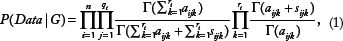29 but also because Zabell³² proved that if we make certain assumptions about an individual's beliefs, then that individual must use the Dirichlet density function to quantify any prior beliefs about a relative frequency. In the case of discrete distributions, the Bayesian score is as follows:

P (D a t a | G) = \prod_{i = 1}^{n} \prod_{j = 1}^{q_{t}} \frac{Γ (\sum_{k = 1}^{r_{t}} a_{i j k})}{Γ (\sum_{k = 1}^{r_{t}} a_{i j k} + \sum_{k = 1}^{r_{t}} s_{i j k})} \prod_{k = 1}^{r_{t}} \frac{Γ (a_{i j k} + s_{i j k})}{Γ (a_{i j k})},

(1) where r_i is the number of states of X_i, q_i is the number of different instantiations of the parents of X_i, a_ijk is the ascertained prior belief concerning the number of times X_i took its kth value when the parents of X_i had their jth instantiation, and s_ijk is the number of times in the data that X_i took its kth value when the parents of X_i had their jth instantiation. The parameters a_ijk are known as hyperparameters. When using the Bayesian score we often determine the values of the hyperparameters a_ijk from a single parameter α called the prior equivalent sample size.³³ If we want to use a prior equivalent sample size α and represent a prior uniform distribution for each variable in the network, for all i, j, and k, we set a_ijk = α / r_iq_i. In this case, the Bayesian score is called the Bayesian Dirichlet uniform equivalent (BDeu) score.

To learn a DAG from the data, we can score all DAGs using the BDeu score and then choose the highest scoring DAG. However, if the number of variables is not small, the number of candidate DAGs is forbiddingly large. Furthermore, the BN model selection problem has been shown to be NP-hard.³⁴ Thus, heuristic algorithms have been developed to search over the space of DAGs during learning.¹⁹

An ID is a BN augmented with decision nodes and a utility node. An ID not only provides us with probabilities of variables of interest but also recommends decisions based on the patient's preferences. Figure 2 shows an ID modeling the decision of whether to be treated with a thoracotomy for a non-small-cell carcinoma of the lung, taken from Ref. 35. The circular nodes are chance nodes, as in BNs. An edge into a chance node is called a relevance edge. The rectangular nodes are decision nodes. An edge into a decision node is an information edge and represents what is known when the decision is made. The diamond-shaped node is a utility node, and represents the utility of the outcomes to the patient. Edges into this node represent features that directly affect this utility.

Figure 2.

An ID modeling the decision of whether to be treated with a thoracotomy for a non-small-cell carcinoma of the lung.

Algorithms for solving IDs determine the decision that maximizes expected utility.¹⁹ The ID in Figure 2 is solved and the expected utility of the first decision (CT scan) is shown in that node.

EBMC

Next, we introduce the BN-based EBMC algorithm used by our survival prediction method.

EBMC Algorithm.

Ideally, if we want to use causes to predict an effect such as survival status, we would want to make all the causes parents of the effect in a BN, and use that network for our predictions. However, unless there are few causes, we do not have the data to learn such a network. For example, if all variables are binary and we have only 10 variables, there are 1024 combinations of values of the causes. An approach often taken to circumvent this dilemma is to make the causes children of the effect. Such a network is called a naive Bayesian network (naive BN),²³ and has sometimes been shown to have good results.³⁶ However, there is a problem with this approach. That is, it makes the wrong conditional independency assumptions. That is, it assumes the causes are conditionally independent given the effect, whereas in actuality, they are conditionally dependent given the effect (due to what psychologists call discounting). As a result, naive BNs have sometimes yielded very poor results.³⁷

EBMC¹⁷ builds on the naive BN approach, but ameliorates the difficulty just mentioned. We discuss how EBMC scores candidate models after illustrating its search algorithm using an example. Figure 3 shows an example of the search. The algorithm starts by scoring all DAG models in which a single predictor is the parent of the target node T The model containing the highest scoring predictor is our initial model as shown in Figure 3(a), where we have labeled the predictor C₁ We then determine which predictor, when added as a parent of T to this 1-predictor model, yields the highest scoring 2-predictor model. If that 2-predictor model has a higher score than our 1-predictor model, our new model becomes the 2-predictor model as depicted in Figure 3(b). We keep adding predictors to the model as long as we can increase the score. When no predictor increases the score further, we search for a predictor that on deletion increases the score, and delete the predictor whose deletion increases the score the most. We continue deleting predictors until no predictor deletion further increases the score. Note that in theory, we could skip the forward search and start the backward search with the complete DAG (one with an edge between every pair of nodes). The problem in starting from the complete model is that for most realistic domains, the number of parameters in the model will be prohibitively large. The hope is that the forward search will identify a model that is as simple as possible.

Figure 3.

An example illustrating the EBMC search.

Suppose our final model is the one in Figure 3(b). We then make the predictors in the model children of T and create edges between them. The edges can go in any direction as long as we do not create a cycle. The result is the model in Figure 3(c). By doing so, we have not introduced any new conditional independencies. Thus, the model in Figure 3(c) can represent all the probability distributions that can be represented by the model in Figure 3(b). This means both models will make the same predictions concerning T.

Next, the search continues in the same manner identifying additional predictors. That is, we first identify the single predictor that when added as a parent of T to the model in Figure 3(c) increases the score of that model the most. We again proceed with forward and backward search. Suppose the search yields one additional predictor. We then have the model in Figure 3(d). In the same way as before, we make the new predictors children of T and create edges between them. The result appears in Figure 3(e). The search repeatedly continues in this manner until we cannot increase the score further. The final model learned is used to perform inference. The network produced by EBMC is called an augmented naive BN³⁸ because there can be edges between the children.

EBMC scores models using the BDeu score in conjunction with the supervised (prequential) scoring method described in Ref. 39. This scoring method evaluates how well the predictor variables (both parents and children) predict the target variable rather than focusing on learning an overall most probable model.

Note that even if all the predictors are fully observed, EBMC does not make the same prediction as the naive BN model. For example, suppose we have the network in Figure 3(c) and we are computing 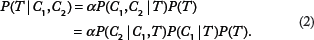P(T| C₁, C₂). This computation would be done using Bayes’ theorem as follows:

\begin{matrix} P (T | C_{1}, C_{2}) = α P (C_{1}, C_{2} | T) P (T) \\ = α P (C_{2} | C_{1}, T) P (C_{1} | T) P (T) . \end{matrix}

(2) where α is a normalizing constant. The naive BN model would estimate P(C₂ | C₁, T) by P(C₂ |T), whereas EBMC does not.

Time Complexity of EBMC.

The time complexity of the EBMC search is O(rs² mn), where r is the total number of rules learned for the model (two in the example above), s is the maximum number of parents of node D in any rule in the model (two in the example), n is the total number of potential predictors, and m is the number of records in the dataset. Ordinarily, r and s values are small compared to m and n; thus the run time is dominated by the size of the dataset, which is mn. Any algorithm that considers all the data would require time that is at least proportional to mn.

EBMC Handles High-Dimensional Data.

The EBMC algorithm has been shown to be capable of handing high-dimensional datasets. In Ref. 17, it was used to predict late onset Alzheimer's disease (LOAD) using a genome wide association study (GWAS) dataset containing 312,316 single nucleotide polymorphisms (SNPs).⁴⁰ In a 5-fold cross-validation analysis, EBMC predicted LOAD risk with an area under the ROC curve (AUROC) equal to 0.728.

Predicting Survivorship Using EBMC.

We model survivorship by discretizing the survival time into whole years. We then use EBMC to learn a separate prediction model for each year. We call the resultant method for predicting survivorship EBMC_Survivorship (EBMC_S). Predicting survivorship by treating each year as a separate prediction problem is a new strategy and, as we shall see in the Results section, has advantages in the patient survival prediction problem.

We evaluated EBMC_S using the METABRIC dataset,¹⁸ which concerns primary breast tumors. There are 981 patients included in this dataset. We first transformed the METABRIC dataset using a combination of domain knowledge and equal distribution discretization strategy. We discuss that transformation next.

Transforming the Dataset.

Table 1 shows the variables and their values used in our analysis. We discuss only the variables whose values we transformed from their original METABRIC values.

Table 1.

The variables used to predict survival.

VARIABLE	DESCRIPTION	VALUES
Age_at_diagnosis	Age at diagnosis of the disease	0–39
		39–54
		54–69
		69–84
		84–100
Size	Size of tumor in cm	0–20
		20–50
		50–180
Lymph_nodes_positive	Number of positive lymph nodes	0
		1
		2–3
		4–5
		6–9
		≥ 10
Grade	Grade of disease	1
		2
		3
Histological	Tumor histology	IDC
		IDC + ILC
		IDC - TUB
		IDC - MUC
		IDC - MED
		Mixed NST and a special type other
		Other invasive
		Invasive tumor
ER_IHC_status	ER status	+
ER_IHC_status	ER status	-
ER_Expr	Estrogen receptor expression	+
ER_Expr	Estrogen receptor expression	-
PR_Expr	Progesterone receptor expression	+
PR_Expr	Progesterone receptor expression	-
HER2_IHC_status	HER2 status	1
		2
		3
HER2_SNP6_state	HER2 copy number gain or loss	Neut
		Gain
		Loss
HER2_Expr	HER2 expression	+
HER2_Expr	HER2 expression	-
RT	Treatment	None
		HT
		RT
		CT
		HT/RT
		HT/CT
		RT/CT
		HT/RT/CT
Inf_men_status	Inferred menopausal status	Pre Post
Group	Characterizes patients by lymph node status and chemo- and hormonal therapy	1
		2
		3
		4
		Other
Stage	Composite of size and number of positive lymph nodes	Numeric
Lymph_nodes_removed	Number of lymph nodes removed	Numeric
NPI	Nottingham Prognostic Index, a composite of tumor size, number of positive lymph nodes, and grade	Numeric
Cellularity	Cells seen on histopathology	High
		Low
		Moderate
P53_mutation_status	Whether P53 is mutated	MUT
P53_mutation_status	Whether P53 is mutated	WT
P53_mutation_type	Type of P53 mutation	Frameshift
		Missense
		Missense: truncating
		Truncating
Pam50_subtype	subtype inferred from expression data	Basal
		Her2
		LumA
		LumB
		NC
		Normal
Int_clust_memb	Cluster membership according to METABRIC	1
		2
		3
		4
		5
		6
		7
		8
		9
		10
Site	Collection site information specific to METABRIC	1
		2
		3
		4
		5
Genefu	A composite of other variables used by METABRIC	ER+/HER2-
		High prolif
		Low prolif
		ER-/HER2-
		HER2+

age_at_diagnosis: we discretized this variable to the ranges shown based on a combination of the equal distribution discretization technique and breast cancer expert knowledge.

size: we discretized this variable to the three standard ranges shown.

lymph_nodes_positive: we grouped this variable into the shown six ranges.

Furthermore, the dataset has the following two fields:

day: this field denotes the number of days.

status: this field's value is dead if the patient died day number of days after the initial consultation, and its value is aliveif the patient was last seen day number of days after initial consultation (and therefore was known to be alive at that time).

Any patient whose status field contains the value alive is right censored. We created a table as shown in Table 2. Patient 2 was found to be dead in Year₂. Thus Year₂ and all subsequent years in Table 2 have value dead. Patient 3 was last seen in Year₂, and was alive. Thus we do not know the status of Patient 3 in the subsequent years, and this patient is right censored.

Table 2.

A table developed from the METABRIC dataset.

PATIENT X₁ X₂ … X₂₄	YEAR₁	YEAR₂	YEAR₃	… YEAR₁₄	YEAR₁₅
1	Alive	Alive	Alive	Alive	Alive
2	Alive	Dead	Dead	Dead	Dead
3	Alive	Alive	-	-	-
…

Evaluation Methodology.

We compared the prediction performance of EBMC_S to that of the standard Cox proportional hazards model⁵ and the RSF¹⁰ method using the METABRIC dataset.¹⁸ We chose the RSF method because it was recently shown to significantly outperform both the Cox model and a newly develop k-nearest neighbors method.¹¹ We used multivariate imputation by chained equations (MICE)⁴¹to impute missing values. Using 5-fold cross-validation, we evaluated models that look 5, 10, and 15 years into the future.

Results

Table 3 shows the concordance indices with 95% confidence intervals for EBMC_S, the Cox proportional hazards model, and the RSF method. Table 4 shows the results of significance testing for EBMC_S versus those for the other two methods. EMBC_S performed significantly better than the Cox model in all the 3 years investigated, with the difference more noteworthy when we looked 5 or 10 years into the future. EBMC_S significantly outperformed the RSF method at 15 years, while the RSF method significantly outperformed EBMC_S at 5 years. Although EBMC_S outperformed the RSF method at 10 years, the result was not significant at the 0.05 level.

Table 3.

Concordance indices with 95% confidence intervals for EBMC_S, the Cox proportional hazards model, and the RSF method.

METHOD	5 YEAR	10 YEAR	15 YEAR
EBMC_S	0.666	0.688	0.688
EBMC_S	(0.637, 0.696)	(0.660, 0.717)	(0.658, 0.718)
Cox	0.620	0.647	0.671
Cox	(0.576, 0.665)	(0.603, 0.692)	(0.625, 0.717)
RSF	0.687	0.686	0.663
RSF	(0.658, 0.717)	(0.657, 0.714)	(0.633, 0.693)

Table 4.

Significance testing results for EBMC_S versus the Cox proportional hazards model and the RSF method.

METHOD	5 YEAR	10 YEAR	15 YEAR
Cox	EBMC_S > Cox; P < 0.05	EBMC_S > Cox; P < 0.05	EBMC_S > Cox; P < 0.05
RSF	EBMC_S < RSF; P < 0.05	EBMC_S > RSF; P = 0.078	EBMC_S > RSF; P < 0.05

The superior performance of EBMC_S relative to the Cox model is likely due to a number of factors including the following: (1) EBMC_S does not make linearity assumptions, but rather naturally models non-linear interactions. For example, survival risk is higher for young and old patients than it is for the middle-aged patients. EBMC_S can capture this with its non-linear modeling. (2) EBMC_S does not make a proportional hazard assumption, but rather looks at each year separately. EBMC_S only performed slightly better than the Cox model when we looked 15 years into the future. However, its performance was still as good as its 10 year prediction performance. On the other hand, the RSF method exhibited its worst performance when we looked 15 years into the future.

Figure 4 shows the ROC curves for EBMC_S for predictions at 1, 5, 10, and 15 years; and Figure 5 shows the AUROCs for all 15 years plotted as a function of the year. We see that, in general, prediction improves as the number of years into the future increases. The result is initially unintuitive because ordinarily we would expect to be able to predict closer events better than more distant events. However, in the case of breast cancer survival, it seems that we can predict whether the person will survive the cancer (15 year prediction) fairly well, but we cannot as readily predict how long those who do not survive the cancer will live.

Figure 4.

ROC curves for 1, 5, 10, and 15 year predictions.

Figure 5.

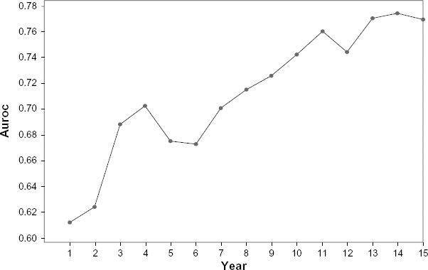
AUROCs plotted as a function of year.

Figure 6 shows the models studied by EBMC_S for 1, 5, 10, and 15 year predictions, when using the entire dataset to study the model. We see that the predictors for the various years are similar but not identical. It is notable that age is a predictor only for long-term survival. It is not surprising that age predicts the long-term survival since we are modeling all-cause mortality; however, it is interesting that age does not seem to predict short-term survival. These results indicate obtaining a separate prediction model for each year individually has advantages in the patient survival prediction problem over models that ascertain a global prediction model for all years.

Figure 6.

Models learned by EBMC_S for 1, 5, 10, and 15 year predictions.

Discussion

We have obtained results indicating that the BN-based EMBC_S algorithm predicts patient survivorship better than the Cox proportional hazard model and comparable to the RSF method. EBMC significantly outperformed the Cox model but did not significantly outperform the RSF method. However, the fact that it performed as well as one of the best current prediction methods is important for several reasons.

First, because EBMC can handle high-dimensional data (as discussed at the end of the EBMC section), EBMC_S can be extended to predict patient survivorship based not only on clinical features but also on high-dimensional genomic dataset. Second, because EBMC_S is BN based, it can readily be incorporated into a complete CDSS that recommends decisions for patients based on their preferences. These two capabilities enable us to make EBMC_S a key component of new generation CDSSs.

EBMC_S has other capabilities not found in many survivorship prediction methods. First, we can perform a sensitivity analysis²⁰ concerning each predictor in the BN learned by EBMC. For example, considering the BN in Figure 6(a), we can determine how sensitive P(Year₁) is, for example, toHER2_Expr by computing the following using a BN inference algorithm:

\frac{P (Y e a r_{1} = d e a d | H E R 2_E x p r = +)}{P (Y e a r_{1} = d e a d)}

(3)

\frac{P (Y e a r_{1} = d e a d | H E R 2_E x p r = -)}{P (Y e a r_{1} = d e a d)} .

(4)

If we have current Evidence about a given patient but do not know the value of HER2_Expr, we can estimate the impact of obtaining this information by computing the following:

\frac{P (Y e a r_{1} = d e a d | H E R 2_E x p r = +, E v i d e n c e)}{P (Y e a r_{1} = d e a d | E v i d e n c e)}

(5)

\frac{P (Y e a r_{1} = d e a d | H E R 2_E x p r = -, E v i d e n c e)}{P (Y e a r_{1} = d e a d | E v i d e n c e)} .

(6)

Second, we can learn which covariates predict survival for a given year. They are not identical for all years.

Third, we can obtain an AUROC for each individual year. Future research can investigate how these AUROCs can be combined with the sample size to predict the measure of confidence in the prediction for each year.

A purpose of this investigation was to make progress toward the development of new generation CDSSs that can make predictions from whatever data are available for a particular patient, inform the physician as to the probable outcomes of treatment options, and make decisions based on the patient's preferences. Next, we plan to expand the breast survival prediction component to include genomic data using the Cancer Genome Atlas (TCGA) database. TCGA is a comprehensive and coordinated effort to accelerate our understanding of the molecular basis of cancer through the application of genome analysis technologies, including large-scale genome sequencing. TCGA makes available breast cancer data from 899 patient tumor samples and 920 matched normal samples, and includes 95 clinical features, 1,561,140 SNPs, 27,578 methylation features, 17,815 gene expression features, 239,323 RNA sequence features, and 1046 miRNA sequence features. Clinical data include demographic features, such as the age at initial pathological diagnosis; diagnostic features, such as diagnosis subtype, histological subtype, tumor size, tumor stage, tumor focality, cellularity, metastasis status, neoplasm disease lymph node status, and HER2/neu positive status; treatment features, such as surgery; and patient outcomes, such as survival. Our resultant prediction system could be used to make survival predictions based on whatever data are available, whether it is clinical data, genomic data, or both. Furthermore, the system could be used to predict how treatment interventions could affect survival status. Eventually, we plan to extend the BN model to an ID model, which not only makes predictions but recommends decisions based on the preferences of the patient.

Conclusion

We conclude that our study supports that EBMC_S can predict patient survivorship better than the Cox proportional hazard model as well as the RSF method. Furthermore, EBMC_S can be extended to predict patient survivorship based not only on clinical features but also on the high-dimensional genomic dataset, and can be readily incorporated into a new generation CDSS that recommends decisions for patients based on their preferences.

Author Contributions

XJ conceived and designed the experiments. DX analyzed the data. RN wrote the first draft of the manuscript. XJ contributed to the writing of the manuscript. AB and SK agreed with the manuscript results and conclusions. RN and XJ jointly developed the structure and arguments for the paper. AB and SK made critical revisions and approved the final version. All authors reviewed and approved the final manuscript.

Disclosures and Ethics

As a requirement of publication the authors have provided signed confirmation of their compliance with ethical and legal obligations including but not limited to compliance with ICMJE authorship and competing interests guidelines, that the article is neither under consideration for publication nor published elsewhere, of their compliance with legal and ethical guidelines concerning human and animal research participants (if applicable), and that permission has been obtained for reproduction of any copyrighted material. This article was subject to blind, independent, expert peer review. The reviewers reported no competing interests.

References

Koboldt

D.C.

, Fulton

R.S.

, McLellan

M.D.

. Comprehensive molecular portraits of human breast tumors. Nature. 2012; 490(7418): 61–70.

Musen

M.A.

, Shahar

, Shortliffe

E.H.

Clinical decision-support systems. In: Shortliffe

E.H.

, Cimino

, eds. Computer Applications in Health Care and Biomedi-cine. New York, NY: Springer; 2006: 698–736.

Wyatt

, Altman

Commentary: prognostic models: clinically useful or quickly forgotten.

Br Med J. 1995; 311: 1539–41.

Nev

, Chin

, Fridlyand

. A collection of breast cancer cell lines for the study of functionally distinct cancer subtypes. Cancer Cell. 2007; 10: 515–27.

Cox

D.R.

Regression models and life-tables.

J R Stat Soc B. 1972; 34(2): 187–220.

Therneau

T.M.

, Grambsch

P.M.

Modeling Survival Data: Extending the Cox Model. New York, NY: Springer; 2000.

Aalen

O.O.

A linear regression model for the analysis of life times.

Stat Med. 1989; 8: 907–25.

Bou-Hamad

, Larocque

, Ben-Ameur

A review of survival trees.

Stat Surv. 2011; 5: 44–71.

Hothorn

, Lausen

, Benner

, Radespiel-Troger

Bagging survival trees.

Stat Surv. 2011; 5: 44–71.

10.

Ishwaran

, Kogalur

U.B.

, Blackstone

E.H.

, Lauer

M.S.

Random survival trees.

Ann Appl Stat. 2008; 2(3): 77–91.

11.

Lowsky

D.J.

, Ding

, Lee

D.K.K.

. A k-nearest neighbors survival probability prediction system. Stat Med. 2012; 32(12): 2062–9.

12.

Ludin

, Lundin

, Burke

H.B.

. Artificial neural networks applied to survival prediction in breast cancer. Oncology. 1999; 57(4): 281–6.

13.

Jayasurya

, Fung

, Yu

, Dehing-Oberije

. Comparison of Bayesian network and support vector machine models for two-year survival prediction in lung cancer patients treated with radiotherapy. Med Phys. 2010; 37(4): 1401–7.

14.

Sierra

, Larrañaga

Predicting survival in malignant skin melanoma using Bayesian networks automatically induced by genetic algorithms. An empirical comparison between different approaches.

Artif Intell Med. 1998; 14(1-2): 215–30.

15.

Heckerman

, Horvitz

, Nathwani

Toward normative expert systems: Part I. The Pathfinder project.

Methods Inf Med. 1992; 31: 90–105.

16.

Lucas

P.J.

, van der Gaag

L.C.

, Abu-Hanna

Bayesian networks in biomedicine and health-care.

Artif Intell Med. 2004; 30(3): 201–14.

17.

Cooper

G.F.

, Yeomans

P.H.

, Visweswaren

, Barmada

An efficient Bayesian method for predicting clinical outcomes from genome-wide data.

In: Proceedings of the AMIA 2010; Washington, D.C.

18.

Curtis

, Shah

S.P.

, Chin

S.F.

. The genomic and transcriptomic architecture of 2,000 breast tumours reveals novel subgroup. Nature. 2012; 486: 346–52.

19.

Neapolitan

R.E.

Learning Bayesian Networks. Upper Saddle River, NJ: Prentice Hall; 2003.

20.

Pearl

Probabilistic Reasoning in Intelligent Systems. Burlington, MA: Morgan Kaufmann; 1988.

21.

Neapolitan

R.E.

Probabilistic Reasoning in Expert Systems. New York, NY: Wiley; 1989.

22.

Korb

, Nicholson

A.E.

Bayesian Artificial Intelligence. Boca Raton, FL: Chapman & Hall/CRC; 2003.

23.

Kjaerulff

U.B.

, Madsen

A.L.

Bayesian Networks and Influence Diagrams. New York, NY: Springer; 2010.

24.

Neapolitan

R.E.

Probabilistic Reasoning in Bioinformatics. Burlington, MA: Morgan Kaufmann; 2009.

25.

Segal

, Pe'er

, Regev

, Koller

, Friedman

Learning module networks.

J Mach Learn Res. 2006; 6: 557–88.

26.

Friedman

, Linial

, Nachman

, Pe'er

Using Bayesian networks to analyze expression data.

J Comput Biol. 2000; 7(3-4): 601–20.

27.

Friedman

, Koller

Being Bayesian about network structure: a Bayesian approach to structure discovery in Bayesian networks.

Mach Learn. 2003; 50: 95–125.

28.

Fishelson

, Geiger

Optimizing exact genetic linkage computation.

J Comput Biol. 2004; 11: 114–21.

29.

Jiang

, Neapolitan

R.E.

Mining strict epistatic interactions from high-dimensional datasets: ameliorating the curse of dimensionality.

PLoS ONE. 2012; 7(10): e46771. doi: 10.1371/journal.pone.0046771.

30.

Cooper

G.F.

The computational complexity of probabilistic inference using Bayesian belief networks.

J Artif Intell. 1990; 42(2-3): 393–405.

31.

Cooper

G.F.

, Herskovits

A Bayesian method for the induction of probabilistic networks from data.

Mach Learn. 1992; 9: 309–47.

32.

Zabell

S.L.

W.E. Johnson's ‘sufficientness postulate.’

Ann Stat. 1982; 10(4): 1090–9.

33.

Heckerman

, Geiger

, Chickering

Learning Bayesian networks: the combination of knowledge and statistical data. Technical Report MSR-TR-94-09 1995: Microsoft Research.

34.

Chickering

Learning Bayesian networks is NP-complete. In: Fisher

, Lenz

, eds. Learning from Data: Lecture Notes in Statistics. New York, NY: Springer; 1996: 121–30.

35.

Nease

R.F.

Jr , Owens

D.K.

Use of influence diagrams to structure medical decisions.

Med Decis Making. 1997; 7(3): 263–75.

36.

Sun

, Shenoy

Using Bayesian networks for bankruptcy prediction: some methodological issues.

Eur J Oper Res. 2007; 180(2): 738–53.

37.

Mandel

, Culotta

, Boulahanis

, Stark

, Lewis

, Rodrigue

A demographic analysis of online sentiment during hurricane Irene.

Proceedings of the Second Workshop on Language in Social Media 2012. Montreal, Canada.

38.

Friedman

, Geiger

, Goldszmidt

Bayesian network classifiers.

Machine Learning. 1997; 29: 131–63.

39.

Kontkanen

, Myllymaki

, Silander

, Tirri

On supervised selection of Bayesian networks.

In: Proceedings of the Fifteenth Conference on Uncertainty in Artificial Intelligence; 1999; Stockholm, Sweden.

40.

Reiman

E.M.

, Webster

J.A.

, Myers

A.J.

. GAB2 alleles modify Alzheimer's risk in APOE carriers. Neuron. 2007; 54: 713–20.

41.

van Buuren

, Oudshoorn

Multivariate imputation by chained equations: MICE V1.0 User's manual.

TNO Prevention and Health 2000; PG/VGZ/00.038.

A New Method for Predicting Patient Survivorship Using Efficient Bayesian Network Learning

Abstract

Keywords

Introduction

Method

BNs and Influence Diagrams (IDs).

EBMC

EBMC Algorithm.

Time Complexity of EBMC.

EBMC Handles High-Dimensional Data.

Predicting Survivorship Using EBMC.

Transforming the Dataset.

Evaluation Methodology.

Results

Discussion

Conclusion

Author Contributions

Disclosures and Ethics

References