
Abstract
Background:
Due to the substantial increase in the number of glaucoma cases within the next several decades, glaucoma is a significant public health issue. The main objective of this study was to investigate the determinant factors of intraocular pressure and time to blindness of glaucoma patients under treatment at Felege Hiwot Referral Hospital, Bahir Dar, Ethiopia.
Methods:
A retrospective study design was conducted on 328 randomly selected glaucoma patients using simple random sampling based on the identification number of patients in an ophthalmology clinic at the hospital under the follow-up period from January 2014 to December 2018. A linear mixed effects model for intraocular pressure data, a semi-parametric survival model for the time-to-blindness data and joint modeling of the 2 responses were used for data analysis. However, the primary outcome was survival time of glaucoma patients.
Results:
The comparison of joint and separate models revealed that joint model was more adequate and efficient inferences because of its smaller standard errors in parameter estimations. This was also approved using AIC, BIC, and based on a significant likelihood ratio test as well. The estimated association parameter (α) in the joint model was .0160 and statistically significant (P-value = .0349). This indicated that there was strong evidence for positive association between the effects of intraocular pressure and the risk of blindness. The result indicated that the higher value of intraocular pressure was associated with the higher risk of blindness. Age, hypertension, type of medication, cup-disk ratio significantly affects both average intraocular pressure and survival time of glaucoma patients (P-value < .05).
Conclusion:
The predictors; age, hypertension, type of medication, and cup-disk ratio were significantly associated with the 2 responses of glaucoma patients. Health professionals give more attention to patients who have blood pressure and cup-disk ratio greater than 0.7 during the follow-up time to reduce the risk of blindness of glaucoma patients.
Keywords
Background
Glaucoma is a leading cause of irreversible blindness worldwide and associated with characteristic damage to the optic nerve and patterns of visual field loss due to retinal ganglion cell degeneration. 1 Glaucoma encompasses a group of ophthalmic diseases that are believed to share the common pathophysiology of elevated intraocular pressure and causes irreversible visual loss. 2
IOP is the fluid pressure inside the eye and eye care professionals’ uses tonometer to determine this. Most tonometers are calibrated to measure pressure in millimeters of mercury (mmHg). 3 Ocular hypertension refers to a situation in which the pressure inside the eye is higher than 21 mmHg. Normal eye pressure ranges from 10 to 21 mmHg. 4
Due to the substantial increase in the projected number of glaucoma cases within the next several decades, glaucoma is a significant public health issue. The visual outcome is the major concern of glaucoma patients. 5 At diagnosis, 34% of glaucoma patients are worried about the probability of becoming blind in the future; even if this percentage decreases to 11% at follow-up times. 6 Some studies have been conducted related to glaucoma to determine factors affecting the survival time and longitudinal outcomes separately. 7 A study conducted to determine factors that affect the longitudinal change of IOP using linear mixed model. 8 However, the linear mixed model of longitudinal data and the Cox proportional hazards model for time-to-event data, conducted separately do not consider dependencies or interrelationships between these 2 different data types of responses. 9 Hence, an alternative approach of joint modeling of these 2 types of responses was proposed by several researchers.9-13
Joint models of longitudinal and survival data can incorporate all information simultaneously and provide valid and efficient inferences for the given data. 14 There is scarcity of research conducted previously about joint models of longitudinal variation of IOP and time to blindness of glaucoma patients in the study area. Therefore, this study was aimed to investigate joint determinants of change of IOP and time to blindness of glaucoma patients under treatment at Felege Hiwot Referral Hospital, North-West Ethiopia. The result obtained in this investigation helps glaucoma patients and health professionals as well to reduce the number of people being blind because of glaucoma and related diseases.
Materials and Methods
Description of study area and design
This study was conducted at Felege Hiwot Referral Hospital, Bahir Dar, North West Ethiopia. The area is located 563 km far from Addis Ababa, capital city of the country. This hospital also serves as a referral hospital for the people who are referred from different districts. A retrospective study design was carried out to retrieve relevant information from the medical records of glaucoma patients to address the objective of current investigation.
Source of population and data
The glaucoma patients were the source of population for this study. The data was collected from the medical chart of glaucoma patients in the ophthalmology clinic at the hospital whose follow-ups were January 2014 to December 2018. Both the longitudinal and survival data were extracted from the patient’s chart which contains socio-demographic and clinical information of all glaucoma patients under follow-ups. Hence, the data for current investigation was secondary.
Data collection procedures
Ophthalmologic clinic staff and clinical nurses participated in collecting secondary data from cards of patients and a public health expert was assigned as a supervisor and orientation was given for data collectors about the variables included in the investigation.
Quality of data measurement
The data collection tool was pre-tested before the actual data collection to maintain data quality. The completeness and consistency of questions related to secondary data were checked and pre-tested on 45 sample data and proper amendments were included after getting feedback from the pilot test. Data cleaning was conducted on a daily basis and timely feedback was communicated to the data collectors.
Sample size and sampling procedures
Taking Bahir Dar referral hospital, the division of ophthalmology in eye treatment, the target population for this study was recorded eye patients confirmed at Bahir Dar referral hospital. At the time when data was collected, there were more eye patients which were recorded in the hospital during January 2014 to December 2018. For each patient, blindness from glaucoma of at least 1 eye occurring during the time of observation was considered as an event. A simple random sampling method was employed for selecting a representative sample in which each of the patients had an equal chance of being selected to be part of the study. Using a single proportion formula by taking blindness prevalence 0.41 as the estimate of population proportion (P) from the previous study in Ethiopia, Menelik II Hospital, 15 95% confidence interval, 5% margin of error, and adding 10% considering the possible missing records to compensate. Finally, the total sample size was 328.
Variables in the Study
Response variables
The 2 response variables were measures of IOP in mmHg and the survival time of glaucoma patients. The IOP was measured in millimeters of mercury (mmHg) which was measured every 6 months irrespective of patient visits to the ophthalmology clinic of the hospital and a patient with full follow ups had 11 visits including baseline. The survival time of glaucoma patients is the length of time from follow-up start date until the date of blindness (or censor). Glaucoma patients who stayed alive during study time, lost follow-up, or died by other causes were considered as censored. Therefore, survival time of glaucoma is assumed to be the outcome of interest in the analysis. The survival response, survival time in months, is created by subtracting the date of the entry from the date of the last visit.
Independent variables
The independent variables for this study were gender (Female = 0 and Male = 1), Place of residence (Rural = 0 and Urban = 1), age in years, hypertension (No = 0 and Yes = 1), diabetic disease (No = 0 and Yes = 1), type of medication (Timolol = 0, Timolol with Pilocarpine = 1, Timolol with Diamox = 2, and Timolol with Diamox with Pilocarpine = 3), duration of treatment (Short = 0, Medium = 1, and long = 2), stage of glaucoma (Early = 0, Moderate = 1, and Advanced = 2), cup-disk ratio (≤ 0.7 = 0 and >0.7 = 1).
Data processing and analysis
In this study, R 3.5.3 version software was considered for data analysis. Statistical decision was made at 5% of level of significance.
Statistical Models
Linear mixed effect model
A linear mixed model is a parametric linear model for longitudinal or repeated measures data that quantifies the relationships between a continuous dependent variable and various predictor variables. It extends from the classical linear regression model that takes into account both fixed effect and random effect. The random effect contains subject specific effects and the fixed effect contains the set of predictors that are fixed across the subjects or the same for all subjects. The fixed effect parameters describe the relationships of the predictors to the dependent variable for an entire population and random effects are specific to subjects within a population. Consequently, random effects are directly used in modeling the random variation in the dependent variable. 16 The random effects are not only determining the correlation structure between observations on the same subject but also take account of heterogeneity among subjects, due to unobserved characteristics.
The general linear mixed effects model defined as

Where,
✓ yi is the (
✓ β is a
✓ Xi is a
✓ bi is a
✓ Zi is a
✓ εi is the (
The corresponding assumptions for model are
Survival model
Survival analysis is a collection of statistical procedures for data analysis for which the outcome a variable of interest is time until an event occurs. The term survival analysis applies to techniques in which the data being analyzed is the time the process takes for a certain event of interest to occur. It is most important when there is censoring data as opposed to the use of different statistical methods. It involves the modeling and analysis of data that has a principal end point the time until an event occurs (time-to-event data). By time, it is to mean years, months, weeks, or days from the beginning of follow-up of an individual until an event occurs. To summarize survival data there are 2 functions of central interest namely the survivor function and the hazard function.
Survivor function (S(t))
Let “T” be a random variable associated with the survival times (t), survival times (t) be the realization of the random variable T and f(t) be the underlying probability density function of the survival time t. Then the cumulative distribution function F(t), which represents the probability that a subject selected at random will have a survival time less than some stated value t. The distribution function of T is given by:
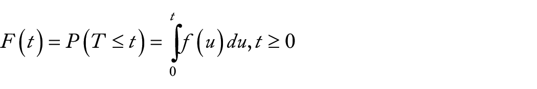
where, F(t) = the probability that a patient gets blind before time t.
The survivor function (S(t)) is defined to be the probability that the survival time of a randomly the selected subject survives beyond some specified time t and so.

Hazard function (h(t))
The hazard function is widely used to express the risk of hazard of death at time t. It is obtained from the probability that an individual dies at time t, given that the individual has survived up to time t. It is also known as the conditional failure rate in reliability, the force of mortality in demography, the intensity function in stochastic process, the age specific failure rate in epidemiology, the inverse of the Mill’s ratio in economics or simply the hazard rate (Hosmer and Lemeshow, 1999). It gives the instantaneous potential per unit time for the event to occur, given that the individual has survived up to time t. The hazard function (h(t)) is given as:

By applying the theory of conditional probability and the relationship in equation, the hazard function can be expressed in terms of the underlying probability density function and the survival function as follows.

A related quantity is the cumulative hazard function H(t) which is defined by:
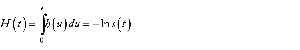
Thus,

Kaplan-Meier (KM)
The Kaplan-Meier (KM) estimator, or Product Limit estimator, is the standard non-parametric estimator of the survival function S(t). It incorporates information from all of the observations available, both censored and uncensored, by considering any point in time as a series of steps defined by the observed survival and censored times. When there is no censoring, the estimator is simply the sample proportion of observations with event times greater than t. The technique becomes a little more complicated, but still manageable when censored times are included.
Suppose
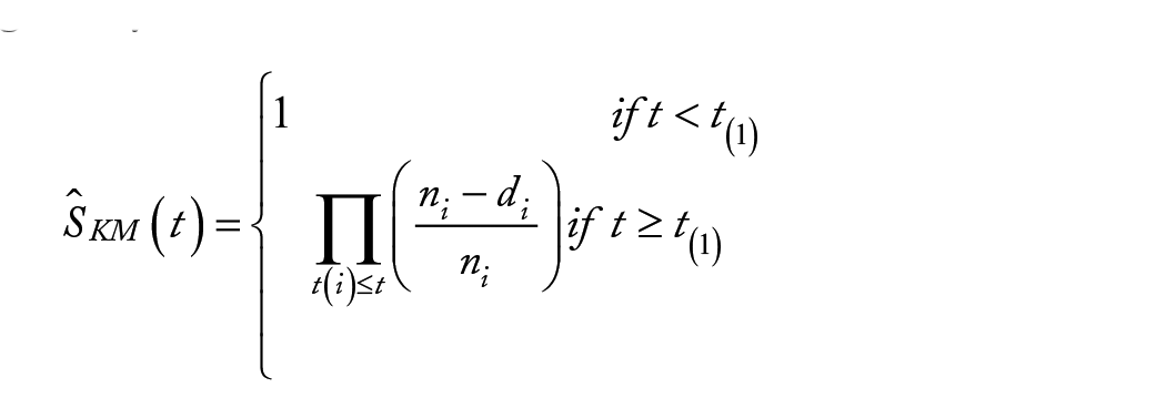
Where,
Log-rank test
The log-rank test, sometimes called the Cox-Mantel test, is the most well-known and widely used test statistic. This test statistic is based on weights equal to 1, that is,
The log rank test was used to compare 2 or more independent survival curves and useful for non-overlapping survival curves. The log rank test statistic for comparing 2 groups is given by:

Cox proportional hazard model
One of the most popular types of regression models used in survival analysis is the Cox proportional hazard model. Although the model is based on the assumption of proportional hazards, no particular form of probability distribution is assumed for the survival times. The model is therefore referred to as a semi-parametric model. The Cox model, a regression method for survival data, provides an estimate of the hazard ratio which is always non-negative and its confidence interval. The hazard ratio is an estimate of the ratio of the hazard rate based on comparison of event rates. The hazard function
Cox (1972) was the first to propose
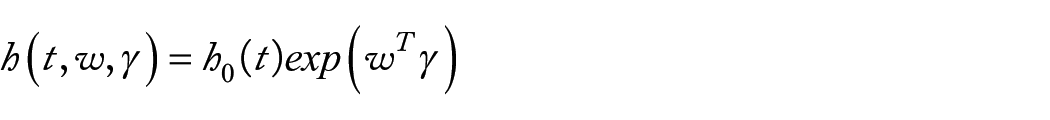
Where,
The ratio of the hazard functions for 2 subjects with covariate values denoted

Therefore, the hazard ratio (
Joint modeling for longitudinal and survival data
In clinical trials, it is common to see repeated measures with time to event which generate both longitudinal data and survival data. One of the natural strategies considering in the joint analysis of longitudinal and survival data is to incorporate the longitudinal measures directly into the Cox PH model as time-varying covariates and then proceed with the Cox proportional hazard model analysis. 17 The intuitive idea behind these models is to couple the survival model, which is of primary interest, with a suitable model for the repeated measurements of the endogenous covariates that will account for its special features. In this situation, a linear mixed effect sub-model was used to model time-varying covariate to address measurement errors (to describe the evolution of the marker in time for each patient) and a Cox proportional hazard sub-model to model the survival data.
Therefore, to examine the impact of the longitudinal outcome to the hazard for an event, an estimate of


where
Results
The patient characteristics of current investigation indicates that among the participants, 108 (32.9%) were females, 146 (45.5%) were from rural area, 98 (29.9%) had hypertension, and 48 (14.6%) were diabetic patients, 65(19.8%), 82(25.0%), 111(33.8%), and 70(21.3%) patients were treated by Timolol, Timolol with Pilocarpine, Timolol with Diamox, and Timolol with Pilocarpine with Diamox respectively. One hundred thirty-five (41.2%), 106 (32.3%), and 87 (26.5%) patients had short treatment duration, medium treatment duration and long treatment duration respectively. One hundred twenty-one (36.9%), 52 (15.9%), and 155(47.3%) had early-stage glaucoma, moderate stage glaucoma, and advanced stage glaucoma respectively. Similarly, 173 (52.7%) of the patients had a maximum of 0.7 cup-disk ratio and the rest 155 (47.3%) of the patients had at least 0.7 cup-disk ratio. Among the total of 328 glaucoma patients, 106 (32.3%) were blind whereas 222 (67.7%) were censored. Among the blind patients, 28 (8.5%) female patients were blind, 74 (22.6%) hypertensive patients were blind, 33 (10.1%) diabetic patients were blind. Similarly, 47 (14.3%) patients who had short term treatment were blind, 45 (13.7%) patients who had medium term treatment were blind, and only 14(4.3%) patients who had long treatment duration were blind. The mean IOP of females and males were 28.29 and 29.92 respectively. The mean age of glaucoma patients at enrollment of ophthalmology clinic was 55.9 years with a standard deviation of 17.4, the youngest patient was 6 years old and the eldest was 89 years old (Table 1).
Characteristics of categorical variables of glaucoma patients.

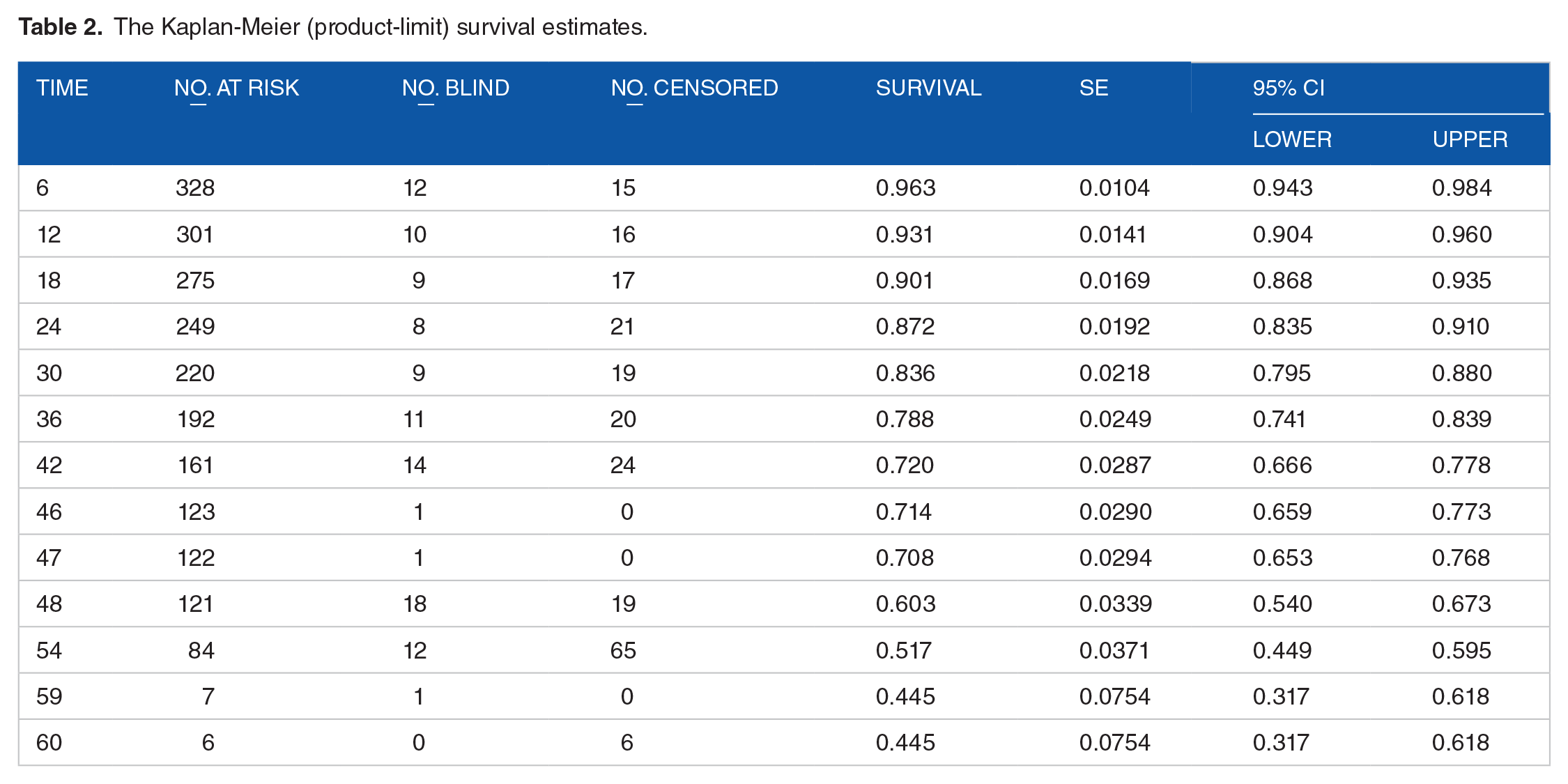
The Kaplan-Meier estimate shows that the median survival time of glaucoma patient was 59 months (Table 2).
The Kaplan-Meier (product-limit) survival estimates.
The Kaplan-Meier survival curves for each study variable provide an initial insight for the shape of survival function. The Kaplan-Meier survival curves to see whether there is a difference in time to blindness between different categories of the covariates. The overall survival curve of glaucoma patients was decreased when the time in months increased (Figure 1).
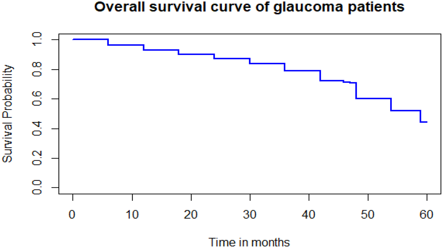
The overall estimate of Kaplan-Meier survival curve of glaucoma patients.
The variables hypertension, diabetic disease, type of medication, duration of treatment, stage of glaucoma, and cup-disk ratio were statistically significant differences between the survival experience (time to blindness) of different groups of glaucoma patients. However, gender and residence there were no survival experience differences between the groups at 5% of level of significance (Table 3).
Results of the log-rank test for each categorical variable of glaucoma patients.
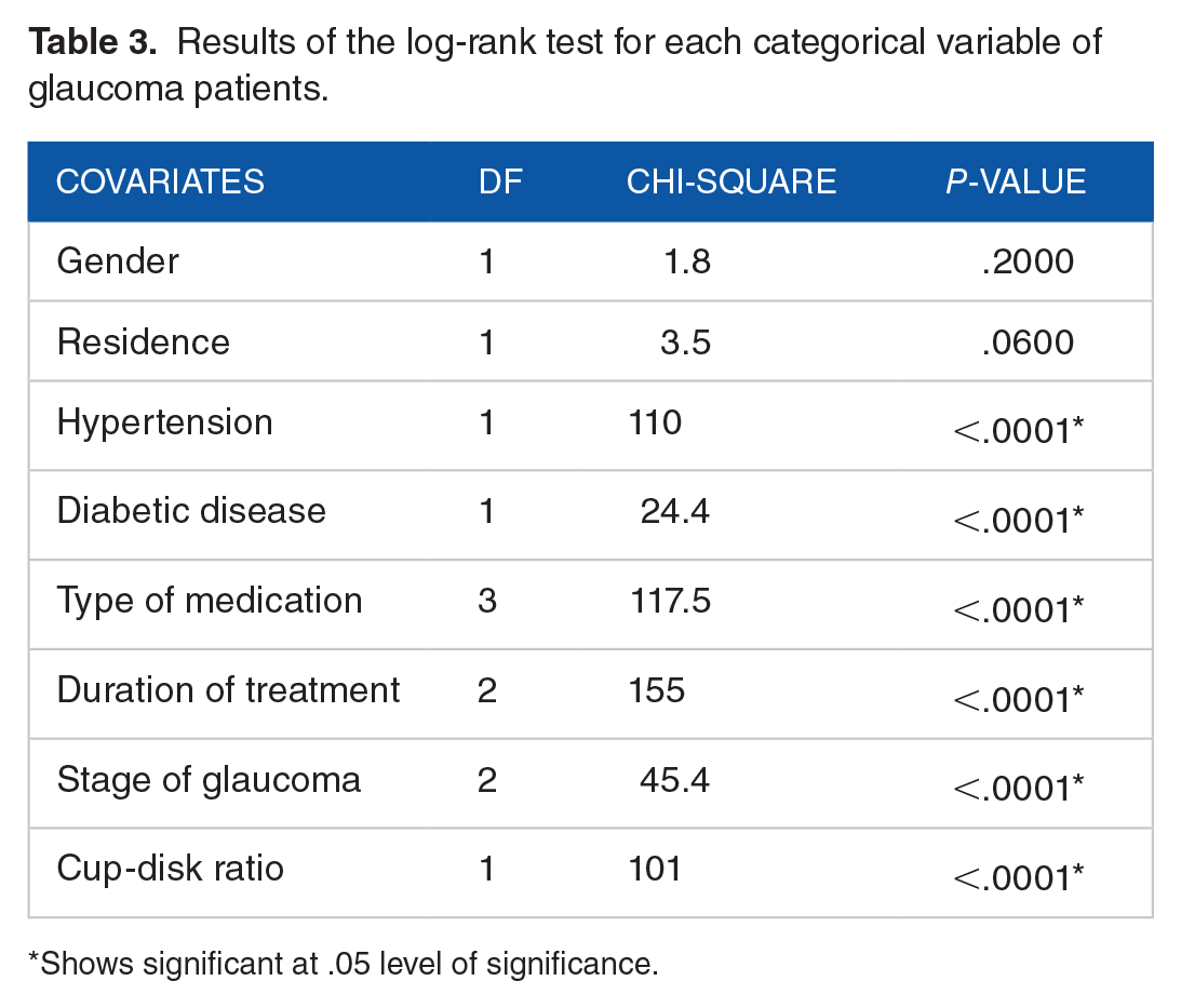
Shows significant at .05 level of significance.
The model with the smallest AIC and BIC value of covariance structure. Therefore, first order autoregressive (AR (1)) covariance structure was selected due to the smallest AIC and BIC compared to the remaining covariance structures (Table 4).
Comparison of covariance structure for linear mixed-effects model.

Bold shows smaller AIC and BIC.
The random intercept and slope model allow the intercept and coefficient to vary randomly among individuals. That means, individual IOP of glaucoma patients vary from visit to visit randomly. Therefore, the random intercept and slope model more parsimonious model for the linear mixed effects model on the basis of its lower values of AIC and BIC (Table 5).
Selection of random effects to be included in the LMM.

Bold shows smaller AIC and BIC.
Univariable analysis for linear mixed model
A univariable analysis was performed in order to see the effect of each covariate on intraocular pressure by using purposeful variable selection in linear mixed effect model analysis and to select variables to be included in the multivariable analysis. Based on univariable analysis all predictors were a candidate variable for multivariable analysis of linear mixed models at 25% level of significance.
Multivariable analysis for linear mixed model
Multivariable analysis of linear mixed model was done by considering all significant covariates at univariable analysis. The result showed that the predictors, age, place of residence, hypertension, type of medication, cup-disk ratio, and visits were significantly associated with the average IOP at 5% of level of significance. Under the random effects result, the estimated subject-specific variability was statistically significant at 5% level of significance (Table 6).
Result of the final linear mixed model for glaucoma patients.

Abbreviation: Ref, reference category.
Shows significant at .05 level of significance.
Univariable analysis for Cox proportional hazard model
The variables which were significant at the P-values less than .25 at univariable analysis were included in the multivariable analysis. The result of the univariable analysis indicated that all predictors were statistically significant at 25% level of significance for Cox proportional hazard model and taken as candidate variables for multivariable analysis.
Multivariable analysis for Cox proportional hazard model
The multivariable analysis of Cox proportional hazard model indicates that the predictors; age, hypertension, diabetic disease, duration of treatment, and cup-disk ratio were significantly associated with time to blindness of glaucoma patients at 5% of level of significance (Table 7).
Result of the final Cox proportional hazards model for glaucoma patients.

Abbreviation: Ref, reference category.
Shows significant at .05 level of significance.
In the longitudinal sub model, the estimated coefficient of fixed effect intercept was 25.1515, indicates that the average IOP of the patients was 25.1515 mmHg at baseline time by excluding all covariates in the model (P-value < .0001). For a unit increased in age, the average IOP of the patients was significantly increased by 0.0726 mmHg (P-value < .0001). The average IOP of the patient who lived urban was significantly lower by 1.8443 mmHg (P-value = .0005) compared to the patient who lived in the rural area.
The average IOP of the patient who had hypertension was significantly higher by 4.5076 mmHg (P-value < .0001) compared to the patient who had no hypertension. The average IOP of the patient who take pilocarpine medication were significantly lower by 3.3413 mmHg (P-value = .0041) compared to the patient who take timolol medication and the average IOP of the patient who take timolol with Diamox medication were significantly higher by 2.3838 mmHg (P-value = .0051) compared to the patient who take timolol medication. The average IOP of the patient who had greater than 0.7 cup-disk ratio was significantly higher by 2.9238 mmHg (P-value < .0001) compared to the patient who had less than or equal to 0.7 cup-disk ratio. For a unit increased in the visits (follow-up time), the average IOP of glaucoma patients was significantly decreased by 0.3489 mmHg (P-value < .0001) keeping all other variables constant.
In the survival sub model, for a unit increased in age, the hazard of blindness of glaucoma patients was significantly increased by 2% (P-value = .0020). The risk of blindness of the glaucoma patient who had hypertension was 2.129 (P-value = .0042) times the risk of blindness of the patient who had no hypertension. The risk of blindness of the glaucoma patient who had diabetic disease was 1.564 (P-value = .0478) times the risk of blindness of the patient who had no diabetic disease. The risk of blindness of the glaucoma patient who took pilocarpine medication was 0.645 (P-value = .0110) times the risk of blindness of the patient who took timolol medication. The risk of blindness of the glaucoma patient who had medium duration of treatment and long duration of treatment were 0.036 (P-value < .0001) and 0.0014 (P-value < .0001) times the risk of blindness of the patient who had short duration of treatment respectively keeping all other variables constant. The risk of blindness of the glaucoma patient who had greater than 0.7 cup-disk ratio was 3.732 (P-value < .0001) times the risk of blindness of the patient who had less than or equal to 0.7 cup-disk ratio keeping all other variables constant. The estimate of the association parameter was α = .0160 (P-value = .0349), indicating that there is a positive association between IOP and time to blindness of glaucoma patients. The result indicates that the higher value of IOP was associated with the higher risk of blindness (Table 8).
Result of joint model of longitudinal IOP and time to blindness of glaucoma patients.

Abbreviation: Ref, reference category.
Shows significant at .05 level of significance.
Comparison of separate and joint model
The estimates of the parameters of the separate and joint models are quite similar to each other but not identical. To compare separate and joint models based on standard error computed in the 2 models for significant predictors. The model with smaller standard error is the better fit for the data. When evaluating the overall performance of both the separate and joint models in terms of model parsimony and goodness of fit, the joint model was performed better based on its lower AIC, BIC and based on a significant likelihood ratio test as well. The association parameter being significant was also evidence that the joint model was better fit than the separate models in this study. The residual variability was smaller in joint model analysis as compared to separate model analysis which indicates that the standard errors were adjusted for the correlation between the 2 responses in the joint model.
Discussion
In this study, 3 different models were explored, the linear mixed effects model for longitudinal IOP, Cox proportional hazards model for survival time of glaucoma patients independently, and jointly modeling of the 2 outcomes together.
In this study, the association parameter was statistically significant in the joint model, indicates that the 2 responses were correlated and shows that the joint model is better fit to the data than the separate models. This finding was consistent with another study. 19
Age is an important socio-demographic predictor of IOP and time to blindness implies that the average IOP and risk of blindness increases with increase in age. This result was in line with other studies,20,21 the result shows that higher age was a significant risk factor for blindness of glaucoma patients. This might be older people who live with ocular hypertension due to this reason increase IOP in older age.
The average IOP was found evolving differently between patients who had hypertension and patients who had no hypertension based on the result of separate and joint models. The average IOP is higher for patients who had hypertension compared to patients who had no hypertension. This result was consistent with other studies.8,22
The glaucoma patients treated with a combination of different medications are exposed to increase of IOP and this further leads to blindness as compared to patients treated with only 1 type of medication. The potential reason for this might be the interaction effect of different medication and management problems of such combined treatment by patients. This finding was consistent with another study, 23 the result showed that the use of a single class of glaucoma medication as simple to manage to reduced hazard of blindness and this is due to lack of knowledge by patients about glaucoma disease to take the medication and patients might be careless for managing combine medication due to the disease nature (the disease most of the time is painless). However, the result obtained in the current investigation contradicts with another study. 23 This contradiction might be the difference of knowledge, attitude, and practice of glaucoma patients who took the medication.
The risk of blindness of patients who had a cup-disk ratio greater than 0.7 is higher compared to patients who had a cup-disk ratio less than or equal to 0.7. This finding was consistent with another study, 24 the result showed that increased the incidence of blindness in a larger cup-disc ratio >0.7. The result associated with cup disc-ratio with size of IOP and hardness of being blindness is consistent with previous studies.9,25 The probable explanation is when a cup-disk ratio increased, IOP also increased due to the nature of the disease.
The result shows the significance of the shared parameter that links the 2 processes together in a joint model while also taking into account the association between them and the reduction in the standard error of the parameter estimates and more efficient inferences when compared to separate model estimates. Therefore, the joint model analysis fits the data better compared to the separate models in current investigation. However, the betterment of the joint model in current investigation may not be true in any other studies because of the nature of data collected from the field.
Conclusion
A joint model and the corresponding separate sub models were built using a retrospective data obtained from an ophthalmology clinic of glaucoma patients under the follow-up 2014 to 2018 at Felege Hiwot Referral Hospital, Bahir Dar, Ethiopia. This study addressed the relationship between the repeated measures IOP and time to blindness of glaucoma patients using joint modeling with a linear mixed effects sub model and a Cox proportional hazards survival sub model.
In conclusion, the results of both separate and joint analyses were quite similar but not identical. However, the use of a joint model analysis compared to separate model analysis adjusted for the correlation between the 2 responses indicates that reducing the standard error and efficient inferences can be made using joint model estimates. In the current investigation the predictors; age, blood pressure, type of medication, cup-disk ratio, and visits were jointly and significantly associated with the 2 response variables namely the change of IOP and time to blindness.
Footnotes
Acknowledgements
The authors would like to thank the Amhara Region Health Bureau, Bahir Dar referral hospital, and Ophthalmic clinic staff members at Felege Hiwot Referral Hospital for supporting the study by granting them access to their medical records. They would also like to extend their gratitude to the Bahir Dar University, College of Science and the Department of Statistics for carrying out the research.
Funding:
The author(s) received no financial support for the research, authorship, and/or publication of this article.
Declaration of conflicting interests:
The author(s) declared no potential conflicts of interest with respect to the research, authorship, and/or publication of this article.
Author Contributions
MWM has led the overall activities of the research process such as drafted the proposal, did the analysis, wrote the results, and prepared the manuscript. AST participated on editing, analysis, and critically revised the manuscript for its scientific content. Both authors read and approved the final manuscript.
Ethics Consideration
The authors got an ethical approval certificate from Bahir Dar University Ethical approval committee, Bahir Dar, Ethiopia with Ref≠BDU/55/2018 to use the secondary data related to patients. The Ethical approval certificate obtained in this committee can be attached up on request. Since the data used in the current investigation was secondary, there was no verbal or written consent from the participants.
Availability of Data and Materials
Data are available on reasonable request.