Sage Journals: Discover world-class research

Abstract

In clinical settings, the diagnosis of medical conditions is often aided by measurement of various serum biomarkers through the use of laboratory tests. These biomarkers provide information about different aspects of a patient's health and overall function of multiple organ systems. We have developed a statistical procedure that condenses the information from a variety of health biomarkers into a composite index, which could be used as a risk score for predicting all-cause mortality. It could also be viewed as a holistic measure of overall physiological health status. This health status metric is computed as a function of standardized values of each biomarker measurement, weighted according to their empirically determined relative strength of association with mortality. The underlying risk model was developed using the biomonitoring and mortality data of a large sample of US residents obtained from the National Health and Nutrition Examination Survey (NHANES) and the National Death Index (NDI). Biomarker concentration levels were standardized using spline-based Cox regression models, and optimization algorithms were used to estimate the weights. The predictive accuracy of the tool was optimized by bootstrap aggregation. We also demonstrate how stacked generalization, a machine learning technique, can be used for further enhancement of the prediction power. The index was shown to be highly predictive of all-cause mortality and long-term outcomes for specific health conditions. It also exhibited a robust association with concurrent chronic conditions, recent hospital utilization, and current health status as assessed by self-rated health.

Keywords

Predictive tool for composite endpoint composite endpoint prediction model clinical prediction model risk prediction model

Introduction

Risk scores for the prediction of health outcomes have become useful and indispensable tools for clinical diagnosis. Most of these risk prediction tools are developed to predict outcomes for a specific condition or population and therefore have limited usefulness outside the scope of their intended target. Some, for example, focus on prediction of risk for particular conditions, eg, cardiovascular disease (Framingham Risk Score,¹ Reynolds Risk Score,² QRISK2,³ etc), kidney disease (QKidney⁴), diabetes (ADA Diabetes Questionnaires⁵), and liver disease (MELD,⁶ RWI_c⁷). Others focus on prediction of health outcomes for specific cohorts, eg, pediatric patients (PRISM) and intensive care patients (APACHE,⁸ SAPS II⁹).

Recent work^10,11 has led to the development of risk scores with a more general scope of applicability. These are primarily intended to predict all-cause mortality for the general population, as opposed to specific cohorts. One such instrument is the Intermountain Risk Score (IMRS).¹¹ The IMRS includes test results from the complete blood count (CBC) and the basic metabolic profile (BMP), a panel of tests for assessing metabolic health. It also includes age in its risk model, which is known to be perhaps the strongest predictor of mortality. Therefore it is possible that the predictive power of this risk-assessment tool may, in large part, be due to the inclusion of age as a component of the risk model.

We have developed a statistical tool for producing a holistic measure of overall health. This health status metric (HSM) covers a wider range of tests than the IMRS. It includes results from the CBC, the lipid panel, and the comprehensive metabolic panel (CMP). The latter is an expanded version of the basic metabolic panel, which includes tests of liver function and provides a broader and more extensive assessment of the body's chemical balance and metabolism. The lipid panel provides, among other things, assessment of cardiac risk, which is one of the most prevalent causes of mortality in the United States.¹² In addition, HSM also includes serum biomarkers such as hemoglobin A1c (a measure of blood glucose concentration), phosphorus, and C-reactive protein, which are known to be prognostic indicators of multiple health conditions.^13–16 The HSM also does not use demographic risk predictors (instead, adjusting for them) and, with the exception of blood pressure, is composed entirely of serum biomarkers from common laboratory tests. And with just serum biomarkers, this index demonstrates strong predictive ability for all-cause mortality and multiple endpoint-specific causes of mortality (liver disease, kidney disease, diabetes).

This makes it potentially useful as a tool for prediction of general risk (with mortality as an endpoint). The HSM also correlates strongly with current health status as assessed by self-rated health, concurrent chronic conditions, and recent hospital utilization. It could therefore be used also as a holistic measure of current health status. Because of the HSM's utilization of a wide range of biomarkers spanning multiple organ systems, it may serve as a particularly effective clinical tool for early identification of at-risk individuals who may be asymptomatic at the time of measurement.

Methods

Data source and risk score components

The HSM was developed using the National Health and Nutrition Examination Survey (NHANES) 1999-2002 dataset (n = 3406)¹⁷ and validated using the NHANES 2003-2008 (n = 4670)¹⁸ and NHANES III 1988-1994 (n = 10592)¹⁹ datasets. Survival data used to develop and test the HSM was obtained from the NHANES 1999-2002 and NHANES III Linked Mortality Files. These files are the result of efforts by the NCHS to conduct a mortality linkage of NHANES data to death certificate data found in the National Death Index (NDI). These files provide information about the death status and survival times (up to December 31, 2006) of NHANES 1999-2002 and NHANES III participants. In addition, information about the underlying cause of death (coded under variable UCOD_113) is available in the Linked Mortality Files. Questionnaire data from the continuous NHANES 2003-2008 data was used to examine the relationship between the HSM and a number of self-reported variables: health status, hospital utilization, and diagnoses of diabetes, heart, kidney, and liver disease.

A total of 24 biomarkers were used to develop the HSM. With the exception of blood pressure, all the biomarkers used are blood/serum measurements, most of which come from the CMP, the lipid panel, and the CBC, batteries of blood tests that are commonly performed in clinical settings for diagnostic purposes. Below is a list of the biomarkers classified by type.

•

Blood pressure

•

Comprehensive metabolic panel

—

Waste products [blood urea nitrogen (BUN), creatinine]

—

Electrolytes (sodium, potassium, chloride, bicarbonate, calcium)

—

Proteins (albumin, globulin)

—

Enzymes [bilirubin, alkaline phosphatase (ALP), aspartate aminotransferase (AST), alanine aminotransferase (ALT)]

•

Lipid panel

—

Triglycerides, HDL : total cholesterol ratio

•

Complete blood count

—

White blood cell, red blood cell, and platelet count

—

Hemoglobin, hematocrit

•

Miscellaneous

—

Hemoglobin A1c

—

Phosphorus

—

C-reactive protein

Standardization

Because the biomarkers are measured in a variety of units, they exist on different scales. In order to combine biomarkers of varying units into one unidimensional index, each biomarker's range of measurements is transformed into a relative hazard scale. Cox proportional hazards regression models with smoothing splines²⁰ were used to plot the relationship between each biomarker's levels and mortality (quantified as relative hazard) after adjusting for age, gender, race, income, and body mass index (BMI) (Fig. 1A–C). These plots allow the range of raw measurements for each biomarker to be mapped onto the relative hazard scale. This scale is then divided into 10 equal-sized intervals (strata), representing discrete levels of risk. The lowest stratum is assigned a value of 0 (indicating the lowest risk level) and the highest a value of 9 (highest risk level). This standardization procedure therefore facilitates the transformation of a set of raw biomarker measurements (with a variety of units) into a uniform, ordinal scale of 0-9. These standardized ordinal values have an intuitive appeal because higher values indicate less desirable biomarker levels and lower values indicate healthier biomarker levels. For example, a bicarbonate level of 10 mmol/L (or below) falls into the highest relative hazard stratum and thus gets assigned a standardized value of 9, representing the highest level of risk relative to the population baseline (Fig. 1A). Note that the training dataset (NHANES 1999-2002) was used to fit the smoothing spline-based Cox proportional hazards models described above. The population in this training dataset is large and diverse enough that the relative hazard plots generated may be considered robust approximations of the true relationship between each biomarker's levels and mortality in the general population.

Figure 1.

(A-C) Examples of relative hazard plots used for transformation of raw biomarker measurements onto the relative hazard scale. Each plot represents the multivariate adjusted, spline-smoothed relative hazard estimates as a function of biomarker level.

Health status metric construction

After all the biomarkers have been standardized, the next step involves using the standardized values to construct the HSM. We follow the weighted quantile sum (WQS) methodology outlined by Carrico (2013)²¹ and Gennings (2013).²² The WQS method is a penalized regression technique for high-dimensional, multicollinear data. Briefly, it involves creating a weighted sum of all variables of interest (standardized onto the same scale) and using the resulting composite as a single variable in a regression model. The weights are unknown model parameters that are constrained to be between 0 and 1 and to sum to 1. Using the WQS approach, the HSM is constructed as follows:

H S M = \sum_{i} w_{i} r_{i} (\sum_{i} w_{i} = 1, 0 \leq w_{i} \leq 1)

(1)

In Equation 1), r_i denote the standardized (on the stratified relative hazard scale) values for the biomarkers, and ω_i are the weights associated with each biomarker. The magnitude of the weight associated with a particular biomarker may be seen as an indicator of the strength of its association with mortality (in the presence of the other biomarkers and after adjusting for demographic variables). This association is defined in a Weibull accelerated failure time model as follows:

\log T_{k} = μ + \sum_{i} a_{j} z_{i} + β \sum_{i} w_{i} r_{i} + σ ψ_{k}

(2)

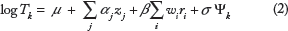
In Equation 2), T_k denotes a random variable associated with the survival time of the kth individual, β is the unknown coefficient of the HSM composite, z_j represent the demographic covariates (age, gender, race, etc), α_jare the unknown coefficients of the z_j, and μ and σ are parameters of the Weibull distribution. Details on how this model is fitted (and the weights estimated) will be discussed in the next section.

Because the standardized biomarker values range from 0 to 9 and the weights add up to 1 and are constrained between 0 and 1, the HSM has the range 0-9. Thus an individual with an HSM score equal to 0 is one who falls into the lowest risk (“healthiest”) stratum on all biomarker measurements, and an individual with an HSM score equal to 9 is one who falls within the highest risk stratum on all biomarkers measured. HSM scores greater than 0 but less than 9 indicate health risk levels falling between these two extremes, with higher scores indicating greater mortality risk.

Estimation of weights

To estimate the weights, the model given in Equation 2) is fitted with data from the NHANES 1999-2002 linked mortality files (training set). In Equation 2), Ψ_k is a random variable used to model the random deviation of log T _k from its expected value according to the model.²³ The equation can be solved to produce an expression for the realization Ψ _k of this random variable:

ψ_{k} = (\log t_{k} - μ - \sum_{j} a_{j} z_{j} - β \sum_{i} w_{i} r_{i}) / σ

The log-likelihood for the Weibull AFT model can then be expressed in terms of Ψ _k :

\log L = \sum_{k} δ_{k} (ψ_{k} - \log σ) - e^{ψ_{k}},

where δ _k is a censoring indicator for the kth individual (0 = assumed alive, 1 = deceased). This log-likelihood function is maximized to obtain estimates for the parameters:

\begin{matrix} \max \log L (σ, μ, {a_{j}}, β, {w_{i}}) \\ [constraints: \sum_{i} w_{i} = 1, 0 \leq w_{i} \leq 1] \end{matrix}

The maximization of this log-likelihood function (subject to the specified constraints) is essentially a constrained nonlinear optimization problem, which was solved numerically using the nonlinear programming procedure (PROC NLP²⁴) in SAS 9.3 (SAS Institute, Cary, NC). The trust region algorithm^25,26 was used with initial values for the weights corresponding to a uniform distribution across all 24 biomarkers used in the analysis (ie, ωi = 1/24, for all i).

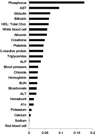
To guarantee stable estimates of the weights, a bootstrap aggregation (“bagging”) technique introduced in Carrico (2013)²¹ was used. A large number (B = 1000) of bootstrap samples (selected with replacement) were generated from the training data, and for each sample b the model defined above was fit to obtain a set of weight estimates ${{\overset{⌢}{ω}}_{i} (b)}_{i = 1}^{24}$ . The weights from all the bootstrap samples b = 1-B were averaged (Fig. 2). These weight estimates were then used to compute the HSM score for any individual with measurements available for all 24 biomarkers:

Figure 2.

Bootstrap-averaged weights used to construct the HSM.

H S M = \sum_{i = 1}^{24} \bar{w_{i}} r_{i}, w h e r e \bar{w} = \frac{1}{B} \sum_{b = 1}^{B} {\hat{w}}_{i} (b)

(3)

Validation

The NHANES III dataset was used as a test/ validation set to assess the predictive strength of the HSM composite. The population in this dataset shares no overlap with the NHANES 1999-2002 population (training set) used to generate the weights for the HSM. These weights were used to compute HSM scores for individuals in the NHANES III dataset. The standardization of the biomarker measurements for NHANES III individuals was carried out using the relative hazard functions computed for the NHANES 1999-2002 population (examples of which are plotted in Figs. 1A–C), rather than recomputing new relative hazard functions specifically for the NHANES III dataset. The rationale behind reusing the NHANES 1999-2002 relative hazard functions is that the eventual goal of this project is to be able to compute the HSM for individual patients without requiring any information about the distribution of biomarker measurements in the populations they belong to. As discussed earlier, due to the large sample size and diversity of the NHANES 1999-2002 dataset, the relative hazard functions computed using this population are robust estimates of the true underlying biomarker-mortality relationships, and are thus suitable for use in the standardization of biomarker measurements of individuals in other datasets.

To test the predictive effect of HSM on survival time in the NHANES III dataset, two methods were utilized. In the first, a Weibull AFT (accelerated failure time) model was used with adjustment for the potentially confounding variables age, gender, race, BMI, and poverty income ratio (PIR). In this validation model, the statistical significance and sign of the HSM coefficient would be indicators of the strength and accuracy of the HSM variable as a predictor for survival time. In particular, since HSM is constructed in such a way that higher values signify worse survival outcomes, a negative and statistically significant HSM coefficient in the validation model would imply that the HSM is a strong predictor of mortality in the test/validation dataset.

The second validation method involved the use of Harrell's C-statistic.²⁷ This statistic can be loosely thought of as the extension of the concept of AUC (area under the ROC curve) to right-censored survival outcomes. Let H be a predictor for a survival outcome, which, for an individual i, assigns a score b _i based on this individual's covariates (x_i). Further, let b _i be such that higher values signify a worse outcome/prognosis. For a pair of individuals (i, j), define this pair as informative if it is possible to know which individual survived longer. Then Harrell's C-statistic is the proportion of informative pairs exhibiting concordance between their prediction scores (b_i;b_j) and their observed survival times (T_i, T_j), where concordance is defined as the case wherein the individual with the higher (worse) score has the shorter survival time, and vice versa. Like AUC, Harrell's C-statistic has a range 0-1, with 0.5 indicating a predictor with no discriminative power and higher values indicating better discriminative power.

As mentioned earlier, the NHANES III Linked Mortality Files also contain information about the cause of death (stored in variable UCOD_113). This information was used to test the ability of the HSM to predict mortality arising from specific chronic illnesses such as cardiovascular disease (codes 053-075), liver disease (codes 093-095), kidney disease (codes 097-101), and diabetes (code 046). Logistic regression (with Firth's bias correction²⁸ for low-prevalence outcomes) was used to test the predictive power of HSM for mortality due to each of these conditions. Age, gender, race, PIR and BMI were adjusted for.

Questionnaire data from participants in NHANES between 2003 and 2008 was used to test the relationship between HSM score and the following self-reported variables: health status, hospital utilization, and diagnoses of diabetes, heart, kidney, and liver disease. Table 1 summarizes the questionnaire items used. Note that the items corresponding to self-reported diagnosis of various heart conditions (items MCQ160B-MCQ160F) were condensed into one variable indicating whether or not a respondent had been notified by their doctor of at least one of these conditions. For the questionnaire variables with binary (Yes/ No) responses, logistic regression was used to model each variable's relationship with HSM while adjusting for age, gender, race, PIR, and BMI. Analysis of the relationship between HSM and questionnaire variables with more than two response categories was carried out using either linear or Poisson regression (see Table 1 for summary), depending on which provided a better fit to the model (as determined by the Akaike information criterion).

Table 1

NHANES 2003-2008 selected questionnaire items and regression techniques used to model their relationship with HSM.

VARIABLE NAME	QUESTIONNAIRE ITEM	NO. OF RESPONSE CATEGORIES	ANALYSIS TECHNIQUE
HUQ010	Self-rated health	5	Linear regression
HUQ050	No. of times healthcare received over past year	6	Poisson regression
HUQ080	No. of times over past year respondent was overnight hospital patient	6	Poisson regression
DIQ010	Doctor ever told respondent they have diabetes?	2 (Yes/No)	Logistic regression
MCQ160L	Doctor ever told respondent they have liver condition?	2 (Yes/No)	Logistic regression
KIQ020	Doctor ever told respondent they have weak/failing kidneys?	2 (Yes/No)	Logistic regression
MCQ160B-MCQ160F	Doctor ever told respondent they have congestive heart failure, coronary heart disease, angina, heart attack, stroke	2 (Yes/No)	Logistic regression

Results

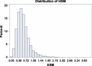
Figure 3 shows the distribution of HSM scores in the NHANES III test/validation population. The HSM demonstrated strong predictive ability (P < 0.0001, ${\hat{β}}_{H S M}$ negative) for all-cause mortality in this validation set. The Harrell's C-measure for the HSM was 0.7.

Figure 3.

Distribution of HSM in NHANES III population.

Figures 4A–F shows a series of Kaplan-Meier curves (adjusted for age and gender) plotted for different HSM ranges. A log-rank test indicates significant difference (P < 0.0001) in survival trends among the strata.

Figure 4.

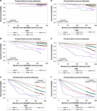
(A) Age, 18-39; gender, female. (B) Age, 40-64; gender, female. (C) Age, ≥65; gender, female. (D) Age, 18-39; gender, male. (E) Age, 40-64; gender, male. (F) Age, ≥65; gender, male.

The HSM also demonstrated high predictive validity for cause-specific mortality (Table 2). The cause-of-death analyses indicated that a 1-unit increase in HSM increases risk of death from liver disease by a factor of ~4, kidney disease by a factor of 2.3, and diabetes by a factor of 2.2.

Table 2

Predictive Validity of HSM (as measured by P-value and odds Ratios [covariate-adjusted]) for death caused by a variety of chronic ailments.

CAUSE OF DEATH	P-VALUE	ODDS RATIO (95% CI)
cardiovascular disease	0.5	0.9 (0.8-1.1)
Liver disease	< 0.0001	3.7 (2.3-6.0)
Kidney disease	0.004	2.2 (1.3-3.7)
Diabetes	<0.0001	2.3 (1.6-3.4)

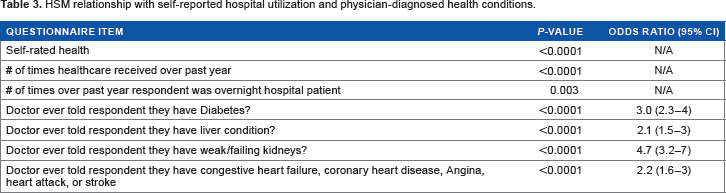
The analysis of items in the NHANES 2003-2008 questionnaire data reveals a robust association between an individual's HSM score and his/her current health status as assessed by self-rated health, self-reported hospital utilization (in the months prior to NHANES participation), and the following self-reported physician-diagnosed health conditions: heart disease, liver disease, kidney disease, and diabetes (Table 3). The results indicate that higher HSM scores are associated with lower self-rated health and more frequent hospital visits. The odds ratio estimates suggest that a 1-unit increase in an individual's HSM score is associated with a 2.6-fold increase in the odds of having been diagnosed with diabetes, a 2.3-fold increase in the odds of having been diagnosed with a liver condition, a 4.5-fold increase in the odds of having been diagnosed with weak/failing kidneys, and 2.3-fold increase in the odds of having been diagnosed with one or more of the following cardiovascular diseases: congestive heart failure, coronary heart disease, angina, heart attack, or stroke. These results should be interpreted with caution. It is tempting to interpret them to mean that increased HSM in any individual is indicative of elevated risk of diabetes, liver, kidney, and cardiovascular disease. However, this would be an incorrect interpretation of the results since they are simply statistical associations observed at the population level. In other words, a particular individual with a relatively high HSM score may not necessarily be at elevated risk for all the aforementioned conditions. The specific conditions (if any) that an individual is at risk of due to relatively high HSM score would depend on their particular biomarker profile. The HSM score should be seen as a predictor of general mortality, not as a predictor of particular illnesses and health conditions.

Table 3

HSM relationship with self-reported hospital utilization and physician-diagnosed health conditions.

QUESTIONNAIRE ITEM	P-VALUE	ODDS RATIO (95% CI)
Self-rated health	<0.0001	N/A
# of times healthcare received over past year	<0.0001	N/A
# of times over past year respondent was overnight hospital patient	0.003	N/A
Doctor ever told respondent they have Diabetes?	<0.0001	3.0 (2.3-4)
Doctor ever told respondent they have liver condition?	<0.0001	2.1 (1.5-3)
Doctor ever told respondent they have weak/failing kidneys?	<0.0001	4.7 (3.2-7)
Doctor ever told respondent they have congestive heart failure, coronary heart disease, Angina, heart attack, or stroke	<0.0001	2.2 (1.6-3)

Table 4

Sample sizes and outcome summaries for datasets used in this study.

DATASET	SAMPLE SIZE	OUTCOME (MORTALITY)
		PERCENTAGE OF CONFIRMED DEATHS	MEDIAN SURVIVAL TIME (MONTHS)
NHANES 1999-2002	3406	4.86%	68
NHANES III (1988-1994)	10592	22.06%	166
NHANES 2003-2008	4670	N/A	N/A

Interpretation of HSM score

HSM scores can be directly translated into projected mortality risk at certain time points in the future. The plots in Figures 5A and B illustrate the relationship between HSM score and probability of mortality 5 years and 10 years, respectively, after HSM score determination. These plots are adjusted for age group and gender, so they can be used to determine an individual's age- and gender-adjusted 5- and 10-year life expectancy based on their present HSM score. Mortality risk at alternate time points can also be easily computed for specific HSM scores.

Figure 5.

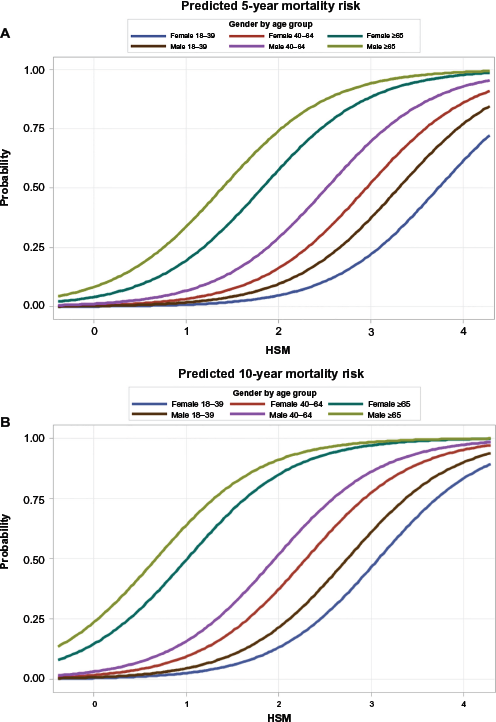
(A) Age- and gender-adjusted relationship between HSM score and 5-year mortality risk. (B) Age- and gender-adjusted relationship between HSM score and 10-year mortality risk.

Predictive power of HSM score

We have demonstrated that the HSM successfully predicts mortality. Its predictive power was assessed using the Harrell's C-statistic and it was found to be of moderate prediction accuracy (C = 0.7). In the construction of the HSM, bagging was used in order to improve the stability of the weight estimates. Bagging is a common data mining technique that is used for improving the performance of predictors.²⁹ It falls under the umbrella of ensemble learning, an approach involving the generation and combination of a large and diverse set of models to produce an “aggregate” model with, among other properties, superior prediction accuracy. While bagging is a powerful technique in its own right, several other ensemble learning techniques exist, and we utilized a particular one (stacked generalization) in an attempt to improve the prediction accuracy of the HSM. Stacked generalization (“stacking”) was originally introduced and characterized in Wolpert,³⁰ and its effectiveness was demonstrated on a neural network. The first documented use of the technique in statistical literature is in Breiman,^31,33 where it was applied to combining regression trees and ridge regression predictors.

In the current study, we applied stacking in order to improve prediction accuracy of the HSM. Like the bagging approach we originally used (described in the Methods section), the first step of stacking involves the generation of a large number of bootstrap samples from the data. To explain subsequent steps of the stacking technique, we begin by reproducing Equation 3) from the Methods section:

H S M = \sum_{i = 1}^{24} \bar{w_{i}} r_{i}, w h e r e \bar{w_{i}} = \frac{1}{B} \sum_{b = 1}^{B} {\hat{w}}_{i (b)}

(3)

Plugging the second expression into the first, we can reformulate the HSM as

H S M = \frac{1}{B} \sum_{b = 1}^{B} H_{b} (r), w h e r e H_{b} (r) = \sum_{i = 1}^{24} {\hat{w}}_{i {(b)}^{r_{i}}}

(4)

H_b(r) above is the particular HSM predictor generated from the bth bootstrap sample. From the reformulation above, it is clear that bagging essentially involves averaging the B HSM predictors ${H_{b} (\cdot)}_{b = 1}^{B}$ that were generated from the B bootstrap samples. The resulting ensemble predictor is called a bagged predictor, which is more stable and often has better predictive performance than that of any of the individual predictors H_b(r). For insights into why bagging, in principle, increases predictive performance, see Ref. 29.

In the stacking technique, the ensemble predictor is created not by averaging the B predictors but by treating them as variables in a model/learning algorithm that estimates the optimal weighting parameters to use to combine them. In stacking terminology, this model is referred to as a meta-model:

\log T_{k} = \sum_{b = 1}^{B} n_{b} H_{b} (r_{k}) + ε

(5)

Here, {n_b} are unknown coefficients, which are estimated by the meta-model; the estimates are the values that best relate the variables ${H_{b} (\cdot)}_{b = 1}^{B}$ to the targeted outcome/response. The end result would be a stacked predictor, ie, the stacking-based HSM:

H S M = \sum_{b = 1}^{B} \hat{n_{b}} H_{b} (r)

(6)

The meta-model defined in Equation 5) is merely for instructive purposes and is actually a somewhat naïve formulation of stacked generalization. In practice, the model as defined in its current form will be ineffective for a number of reasons, the key one being that since the predictors H_b(·) were all constructed from bootstrap samples obtained from the same data, it is reasonable to expect significant correlation among them. Standard regression models such as the one in Equation 5) generally handle multicollinearity poorly. There are a number of well-known modeling techniques for handling multicollinearity (see Bello³² for a discussion of the application of these techniques to stacked generalization). But in the present study, we compared only two: weighted quantile sum (WQS) regression, and partial least squares. We found that WQS performed better, and increased the predictive accuracy (Harrell's C) of the HSM to 0.75. Future studies will focus on improving the prediction power even further.

Conclusion

Using biomarker and survival data, we have developed and validated a composite score that serves a dual purpose as a fairly comprehensive measure of overall health and a prognostic tool capable of predicting mortality risk for the general population.

Validation analysis of the HSM demonstrated that it is both a reasonably accurate gage of current health status and a reliable predictor of life expectancy. Higher HSM scores tend to be linked with lower self-rated health, higher frequency of hospitalization, higher likelihood of chronic health conditions (at present and in the future), and decreased life expectancy.

Nearly all the biomarkers used in constructing the index can be obtained from common laboratory tests (CMP, lipid panel, CBC) performed on patients as part of the diagnosis process or routine checkups. The HSM provides a straightforward way to combine all these markers of various aspects of health into a single score, which serves as a numerical estimate of current overall health and future mortality risk.

Therefore the HSM could potentially be a useful tool in clinical settings for accurately quantifying mortality risk (life expectancy) in individuals with known health issues. HSM would provide clinicians who use it with an evidence-based/ data-driven assessment of general mortality risk that could be used to supplement or substitute the subjective assessments that are sometimes made in clinical practice. And unlike some risk scores that predict mortality only for individuals with a particular disease, the HSM is a general-purpose risk score that could be used to predict mortality for individuals with a wide range of conditions.

HSM could also be used as a measure for tracking a patient's general health over time. Certain longitudinal clinical studies that follow overall health status over time may benefit from the use of a validated, general-purpose risk score such as the HSM.

In healthcare quality assessment studies, HSM could be adapted for use as a metric for comparing patient overall health among different healthcare providers. As an example of such an application, the HSM could be used to obtain estimates of age- and gender-adjusted 5-year life expectancy for patients seen by individual or institutional healthcare providers. These estimates provide a way to make standardized comparisons of patient health outcomes among multiple healthcare providers.

Study limitations

A limitation of the current method of computing HSM is the reliance on a large number of biomarkers (24). While these biomarkers are routinely measured in clinical settings, individual patient health records might be missing one or more components. At this point in time, the computation of the HSM for a patient requires that all 24 biomarkers be available. Future work will focus on developing an adaptive method for computing the HSM in instances when one or more of the biomarkers are missing.

Finally, while the HSM incorporates a wide range of biomarkers spanning multiple organ systems, this range is by no means exhaustive. Certain aspects of overall health (eg, reproductive health, mental health, gastrointestinal health, endocrine function) are not evaluated in a direct manner by the HSM.

Author Contributions

Conceived and designed the experiments: GAB, CG. Analyzed the data: GAB, GGD. Wrote the first draft of the manuscript: GAB. Contributed to the writing of the manuscript: CG, GGD. Agree with manuscript results and conclusions: GAB, GD, CG. Jointly developed the structure and arguments for the paper: GAB, CG. Made critical revisions and approved final version: GAB, CG, GGD. All authors reviewed and approved of the final manuscript.

References

Wilson

P.W.

, D'Agostino

R.B.

, Levy

, Belanger

A.M.

, Silbershatz

, Kannel

W.B.

Prediction of coronary heart disease using risk factor categories. Circulation. 1998; 97: 1837–47.

Ridker

P.M.

, Buring

J.E.

, Rifai

, Cook

N.R.

Development and validation of improved algorithms for the assessment of global cardiovascular risk in women: the reynolds risk score. JAMA. 2007; 297: 611–9.

Hippisley-Cox

, Coupland

, Vinogradova

. Predicting cardiovascular risk in England and Wales: prospective derivation and validation of QRISK2. BMJ. 2008; 336: 1475–82.

Hippisley-Cox

, Coupland

Predicting the risk of chronic kidney disease in men and women in England and Wales: prospective derivation and external validation of the QKidney scores. BMC Fam Pract. 2010; 11: 49–61.

Heikes

K.E.

, Eddy

D.M.

, Arondekar

, Schlessinger

Diabetes risk calculator: a simple tool for detecting undiagnosed diabetes and pre-diabetes. Diabetes Care. 2008; 31: 1040–5.

Kamath

P.S.

, Wiesner

R.H.

, Malinchoc

. A model to predict survival in patients with end-stage liver disease. Hepatology. 2001; 33: 464–70.

Gennings

, Heuman

, Fulton

, Sanyal

A.J.

Use of desirability functions to evaluate health status in patients with cirrhosis. J Hepatol. 2010; 52: 665–71.

Knaus

W.A.

, Wagner

D.P.

, Draper

E.A.

. The APACHE III prognostic system. Risk prediction of hospital mortality for critically ill hospitalized adults. Chest. 1991; 100: 1619–36.

Le Gall

J.R.

, Lemeshow

, Saulnier

A new simplified acute physiology score (SAPS II) based on a European/North American multicenter study. JAMA. 1993; 270: 2957–63.

10.

Gennings

, Ellis

, Ritter

J.K.

Linking empirical estimates of body burden of environmental chemicals and wellness using NHANES data. Environ Int. 2012; 39: 56–65.

11.

Horne

B.D.

, May

H.T.

, Muhlestein

J.B.

. Exceptional mortality prediction by risk scores from common laboratory tests. Am J Med. 2009; 122: 550–8.

12.

Hoyert

D.L.

, Xu

J.Q.

Deaths: preliminary data for 2011. National Vital Statistics Reports. Vol 61. Hyattsville, MD: National Center for Health Statistics; 2012: 6.

13.

Black

, Kushner

, Samols

C-reactive protein. J Biol Chem. 2004; 279: 48487–90.

14.

Goldman

, Schafer

A.I.

Goldman's Cecil Medicine, Chapter 121. 24th ed. Pennsylvania: Saunders Elsevier; 2011.

15.

Luk

A.O.

, Ma

R.C.

, Lau

E.S.

. Risk association of HbA1c variability with chronic kidney disease and cardiovascular disease in type 2 diabetes: prospective analysis of the Hong Kong diabetes registry. Diabetes Metab Res Rev. 2013; 29: 384–90.

16.

Matsushita

, Blecker

, Pazin-Filho

. The association of hemoglobin A1c with incident heart failure among people without diabetes: the atherosclerosis risk in communities study. Diabetes. 2010; 59: 2020–6.

17.

Centers for Disease Control and Prevention (CDC), National Center for Health Statistics (NCHS). National Health and Nutrition Examination Survey Data. Hyattsville, MD: U.S. Department of Health and Human Services, Centers for Disease Control and Prevention; 2002. Available from: http://wwwn.cdc.gov/nchs/nhanes/search/nhanes01_02.aspx.

18.

Centers for Disease Control and Prevention (CDC), National Center for Health Statistics (NCHS). National Health and Nutrition Examination Survey Questionnaire. Hyattsville, MD: U.S. Department of Health and Human Services, Centers for Disease Control and Prevention; 2008. Available from: http://wwwn.cdc.gov/nchs/nhanes/search/datapage.aspx?Component=Questionnaire&CycleBeginYear=2007.

19.

Centers for Disease Control and Prevention (CDC), National Center for Health Statistics (NCHS). National Health and Nutrition Examination Survey Data. Hyattsville, MD: U.S. Department of Health and Human Services, Centers for Disease Control and Prevention; 1994. Available from: http://www.cdc.gov/nchs/nhanes/nh3data.htm.

20.

Therneau

, Grambsch

Modeling Survival Data: Extending the Cox Model. New York: Springer-Verlag; 2000.

21.

Carrico

C.K.

Characterization of a Weighted Quantile Score Approach for Highly Correlated Data in Risk Analysis Scenarios. [Ph.D. Dissertation]. Richmond, Virginia: Virginia Commonwealth University, Department of Biostatistics; 2013.

22.

Gennings

, Carrico

C.K.

, Factor-Litvak

, Krigbaum

, Cirillo

P.M.

, Cohn

B.A.A.

Cohort study evaluation of maternal PCB exposure related to time to pregnancy in daughters. Environ Health. 2013; 12: 66–77.

23.

Collett

Modelling Survival Data in Medical Research. 2nd ed. Boca Raton: CRC Press; 2003.

24.

Institute Inc

S.A.S.

Chapter 7: the NLP procedure. SAS/OR(R) 9.3 Users’ Guide; 2008.

25.

Celis

M.R.

, Dennis

J.E.

, Tapia

R.A.

A trust region strategy for nonlinear equality constrained optimization. Editors: Boggs

P.T.

, Byrd

R.H.

, Schnabel

R.B.

Numerical Optimization 1984. Philadelphia: SIAM; 1985: 71–82.

26.

Moré

J.J.

, Sorensen

D.C.

Computing a trust-region step. SIAM J Sci Stat Comput. 1983; 4: 553–72.

27.

Harrell

F.E.

, Califf

R.M.

, Pryor

D.B.

, Lee

K.L.

, Rosati

R.A.

Evaluating the yield of medical tests. JAMA. 1982; 247(18): 2543–6.

28.

Firth

Bias reduction of maximum likelihood estimates. Biometrika. 1993; 80: 27–38.

29.

Breiman

Bagging predictors. Mach Learn. 1996; 24(2): 123–40.

30.

Wolpert

Stacked generalization. Neural Netω. 1992; 5(2): 241–59.

31.

Breiman

Stacked Regression. Technical Report. Berkeley, CA: Statistics Department, UC Berkeley; 1993.

32.

Bello

G.A.

Application and Extension of Weighted Quantile Sum Regression for the Development of a Clinical Risk Prediction Tool. [Ph.D. Dissertation]. Richmond, Virginia: Virginia Commonwealth University, Department of Biostatistics; 2014.

33.

Breiman

Stacked regressions. Mach Learn. 1996; 24: 49–64.

Development and Validation of a Clinical Risk-Assessment Tool Predictive of All-Cause Mortality

Abstract

Keywords

Introduction

Methods

Data source and risk score components

Standardization

Health status metric construction

Estimation of weights

Validation

Results

Interpretation of HSM score

Predictive power of HSM score

Conclusion

Study limitations

Author Contributions

References