Sage Journals: Discover world-class research

Abstract

Alzheimer’s disease (AD) prediction is a critical task in the field of healthcare, and researchers have been exploring various techniques to improve its accuracy. This research paper focuses on the major contributions of a hybrid deep convolutional neural network (CNN) with denoising using a multilayer perceptron (MLP) and pooling layers in AD prediction. The proposed hybrid model leverages the power of deep CNNs to extract meaningful features from molecular or imaging data related to AD. The model incorporates denoising techniques using MLP to enhance the quality of the input data and reduce noise interference. Additionally, pooling layers are employed to summarize the extracted features and capture their essential characteristics. Several experiments and evaluations were conducted to assess the performance of the proposed model. Comparative analyses were carried out with other techniques such as PCA, CNN, Resnet18, and DCNN. The results were presented in a comparison chart, highlighting the superiority of the hybrid deep CNN with denoising and pooling layers in AD prediction. The research paper further discusses the accuracy, precision, and recall values obtained through the proposed model. These metrics provide insights into the model’s ability to accurately classify AD cases and predict disease progression. Overall, the hybrid deep CNN with denoising using MLP and pooling layers presents a promising approach for AD prediction. The combination of these techniques enables more accurate and reliable predictions, contributing to early detection and improved patient care. The findings of this research contribute to the advancement of AD prediction methodologies and provide valuable insights for future studies in this domain.

Keywords

Alzheimer’s disease prediction hybrid deep CNN denoising MLP pooling layers machine learning and healthcare

1. Introduction

Alzheimer’s disease (AD) is determined a neurologic condition that impairs a patient’s capacity for rational thought, memory, communication, learning new information, and other cognitive skills [1, 2]. Most Alzheimer’s patients are older than 60, generally in their early 60s. Of all physical alterations, brain cell damage is the most severe. The most severely affected brain areas are the amygdala, hippocampus, and a few others that control the majority of the signs of AD [3, 4, 5]. Prior to other grey matter cells being destroyed, learning cells are initially damaged, and leaving the patient unable to carry out even the most fundamental tasks. As a result, those who have Alzheimer’s disease experience severe behavior-related, cognitive, and memory loss [6]. The early 1960s saw AD’s consequences. According to a 2019 “National Institute on Ageing, U.S.A.” study, more than six million Americans have AD [7]. “Alzheimer’s and Dementia Resources” reported that more than four million people in India had AD [8]. The proportion of AD sufferers globally is increasing rapidly and dangerously.

The vast majority of AD patients have reached MCI, the earliest stage of alzheimer [9, 10]. While in a milder form, MCI symptoms are nearly comparable to AD symptoms. The early stages of AD can be referred to as MCI. The majority of individuals with MCI go on to acquire AD, according to a study [10]. Neuron-experts and professionals in psychology perform a variety of psychological and physical tests, involving a health history analyze [11], physical assessment and screening assessments [12], a neurophysiologic evaluation [13], the MMSE [14], an anxiety review [15], and other people. All of these tasks require a variety of tools, which is a lengthy and inefficient procedure.

For acquiring tissue-by-tissue information on the neurological system, the use of MRI, is a common technique [16]. A number of conditions, include cancer, tumours, and others, can be accurately diagnosed by MRI often [17]. Image processing tools can compare cells in AD, MCI, and CN persons. The traditional AD diagnostic method involves a variety of tests, such as physicals, cognitive tests, DNA testing, and so on. The use of brain imaging for AD categorization may be quicker and require fewer tools than the conventional diagnosis method. Additionally, effective brain processing of images may locate important biomarkers years before an individual experiences the onset of Alzheimer’s disease [18]. Conventional image processing methods cannot detect AD due to complicated pixel configurations by analyzing modifications to tissue [19]. The suggested model combines integration methods in machine learning to increase the precision in AD prediction, which is comparable to the data provided above. The following list summarizes the framework’s main contributions:

•
The model employs a multilayer perceptron (MLP) for denoising, which helps to remove noise and enhance the quality of input data. The denoising procedure is essential for increasing the precision and dependability of AD forecasts.
•
The proposed model significantly improves the accuracy of predictions in the context of deep convolutional neural networks (CNN). By incorporating hybridization techniques, it leverages the strengths of different algorithms and architectures, leading to improved performance in AD prediction.
•
The utilization of pooling layers enables the model to perform downsampling and information compression, reducing the computational complexity and improving efficiency. The hierarchical representation of features learned through pooling layers aids in capturing both local and global patterns, leading to improved AD prediction.

2. Related works

Scientists in the medical professions are increasingly using machine learning. The invention of AD identification and forecasting is one topic of intense focus [17]. Machine learning methods, especially those incorporating biological or image information, may diagnose AD. The most recent developments in deep learning frameworks for AD evaluation and forecasting are examined in this article. A DCNNs algorithm for four-class AD identification utilizing MRI images was created by Islam and Zhang [18]. On the OASIS a database, they trained and assessed the Inception-V4 approach, yielding an accuracy of 73.70%. The precision of this mathematical framework was constrained, nonetheless, by the dearth of accessible data. An extremely learning machine -based classification framework for bilateral AD was put out by Zhang et al. [19]. Voxel-based morphology pictures representing 627 patients in the ADNI collection were individually separated.

Shanmugam et al. [20] developed the first transferable learning-based technique for multi-class diagnosis of AD phases and cognitive decline. They developed and evaluated the GoogLeNet, AlexNet, and ResNet-18 networks using 6000 MRI scans from the ADNI collection. The ResNet-18 networks obtained an identification precision of 98.63%, which was the highest. Kong et al. [21] created a specific PET-MRI combining images and a 3D CNN for the deep learning multi-classification of AD. 740 different 3D photos from the ADNI database were used in total. The research suggested utilizing the A3C-TL-GTO algorithm to categorize MRI scans and detect AD. The empirical methodology A3C-TL-GTO for automated and effective AD detection was built and tested using the Alzheimer’s Database (four image classes) and the ADNI.

These papers show how deep learning approaches are still being used to diagnose and predict AD. DCNN, ELM, and model transfers have been tested on imaging databases. These developments aid in the creation of computerized and accurate AD categorization techniques. Alzheimer’s disease (AD) was sourced from publicly available databases such as the Alzheimer’s Disease Neuroimaging Initiative (ADNI), the Australian Imaging, Biomarker & Lifestyle Flagship Study of Ageing (AIBL), and the National Alzheimer’s Coordinating Center (NACC) database. Reduce pre-processing bias and fine-tuning volatility in model classification and information sets using the provided method. It uses MRI-validated methodologies to improve patient care. The research uses MRI brain images from the ADNI’s online Alzheimer’s disease database. Experimental findings show that the recommended strategy is 96.65% accurate on the Alzheimer’s Database and 96.25% accurate on the ADNI Database. The databases’ lack of illustrations raises the possibility of excessive fitting, which reduces the efficiency of models built using deep learning. Orouskhani et al. [22] provide a few-shot learning approach termed deep metrics tracking to overcome this difficulty. They present a unique deep triplet networks that evaluates brain MRIs and detects Alzheimer’s disease via the use of measurement learning. The deep a triplet matrix uses an adaptive function for loss that helps enhance the accuracy of the model and adjust for low data from training. The model’s primary network design depends on the VGG16 system, and tests are carried out utilizing openly accessible imaging research datasets like OASIS. The suggested studies uses the hybrid model for estimating and improve a CNN building layout utilizing a multiobjective functional and several hyperparameters.

3. Proposed methodology for AD prediction

3.1 Preprocessing of data using MLP

Both the real and fake sections of the image are affected by Gaussian distribution noise, which distorts the MR magnitude image. Gaussian noise was added to the input data during training to introduce a controlled level of randomness, encouraging the model to learn more robust and generalizable features. Dropout, on the other hand, was applied within the MLP layers to prevent overfitting and enhance the network’s ability to denoise by training it with partial information. This combination improved the quality of the input data by reducing overfitting and making the model more resilient to noise, ultimately resulting in more accurate and reliable predictions. The probability variation in noisy MRI pixel brightness is a Rician distribution, according to earlier studies. DL can replicate this type of corruption by learning from examples using Multi-Layer Perceptron (MLPs), without considering the underlying physical process. The MLP is trained using the noisy and clean image pairs. The input to the MLP is the noisy image, and the output is the denoised image. During training, the network adjusts its internal parameters (weights and biases) based on the comparison between the denoised output and the corresponding clean image.

$\displaystyle{X}=Y+\delta\left(X\right)$ (1)

The Eq. (1) represents the relationship between the noise-free picture ( $Y$ ) and the noisy MR image ( $X$ ), where ( $X$ ) represents the difference between $X$ and $Y$ influenced by the Rician distribution. By using this equation, a residual mapping, $f(Y;\Theta)$ , was trained to derive $Y=Xf(X;\Theta)$ . Figure 1 shows both the local and global PDF of noise MRI scans. The noise in the upper left picture reduces the MR image’s sharpness and blurs the borders of particular tissue frameworks, making it harder to see finer details. The PDFs of Rician distortion in different physiological areas of cerebral MRI scans vary geographically, according to Liu et al.’s [23] observation. As a result, the nonlinear translations among picture patterns and Rician statistics vary throughout both local and worldwide locations. The 3D-Parallel-RicianNet MR image noise approach, which uses global and local characteristic data from these areas, is our suggested approach.

3.2 Feature extraction using Deep Convolutional Neural Network (DCNN)

The suggested DCNN framework for MR image processing includes three parts: the reconstruction (REC) element, a local feature collection network, and a global feature extracting networks. Figure 1 depicts the pipeline for denoising. DeepCNet and DeepSCNet are used in the beginning stages to extract both regional and global characteristics.

Figure 1.

Denoising cum Feature extraction module.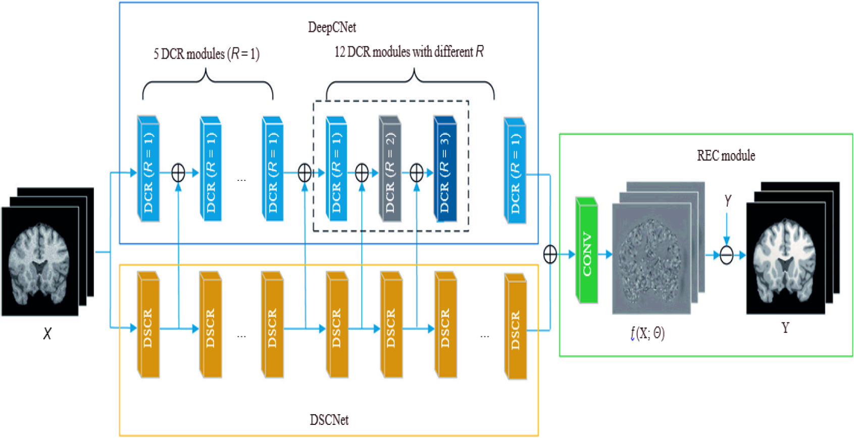

The local as well as global data are then combined using a second layer, producing detailed features that accurately match the properties of the genuine Rician pattern. We produce the anticipated clear magnetic resonance image X using the REC component. The proposed architecture is made up of 18 sequential DCR sections with different R values, collectively called as DCRNet. A kernel size of 33333 is used for 2D slices and 3D patches. Dilated convolution with a high R value proves effective in attenuating low-frequency noise. However, excessively large R values hinder the capture of subtle contextual details, leading to wasted receptive fields. Setting R to 1 ensures each channel retains the same convolution as before. In DeepCNet, we equally pad zeros across borders before convolution to match a map of features size with inputs. As the thickness of the convolutional layers increases, the receptive field size progressively expands. Dilated convolution is associated with a gridding issue, as mentioned in reference [26, 27]. In our investigation, we used DCR units with varying dilatation velocities to solve this issue. The dilation speeds for every layer are individually determined by the following method: 1, 1, 1, 1, 1, 1, 2, 3, 1, 2, 3, and 1 result in a 61-square-meter total reception area. Multiple DCR components with different dilation rates allow multiscale universal feature determination. Each module contains 16 filters, and this implementation helps mitigate the influence of irrelevant information and prevents the occurrence of gridding effects.

3.2.1 DeepSCNet

DeepSCNet compensates for ignored nearby data by widening the receptive area. DeepSCNet’s cascades is made up of 18 DSCR components, for every uses a 3 $\times$ 3 $\times$ 3 convolution kernels and has 16 filtering.

To gradually integrate global and local information, we combine the characteristics gathered from each module of DeepCNet and DeepSCNet. By using this strategy, significant visual characteristics are preserved in both local as well as global areas. As a result, the 3D-Parallel-RicianNet architecture is more effective than previous eliminating techniques. In the pipeline, the REC module is essential. It calculates the estimated deviation, $f(X;\Theta)$ , after a convolution layer, and then utilizes $Y=X+f(X;\Theta)$ MRI.

3.2.2 Loss of function

It measures the discrepancy between the denoised output and the corresponding clean image. Mean squared error (MSE) is a commonly used loss function for image denoising:

$\displaystyle L=1/N\ast\Sigma(||y-\hat{y}||^{2})$ (2)

where: $L$ is the loss value, $N$ be the No. of pixels in the image, $y$ is the clean image and $y$ is the denoised output image.

3.3 Hybridized CNN with Resnet18 taxonomy

We suggest a brand-new CNN algorithm that combines the fundamental ideas of both ResNet and Inception systems. Our approach integrates the ResNet paradigm with the Inception framework utilizing the positive aspects of these two topologies. Previous research has shown that the ResNet and Inception algorithms can manage hundreds of thousands of levels with exceptional effectiveness and performance.

These blocks enable the network to learn residual connections and facilitate training of very deep networks. On the other hand, the Inception model is composed of several convolutional networks that form a deep convolutional network. This architecture allows the model to capture multi-scale features and enhance its representational power.

By combining these concepts, our proposed CNN model aims to leverage the benefits of both ResNet and Inception models, resulting in improved performance and efficiency.

Figure 2.

Proposed hybrid CNN with ResNet18-Inception model.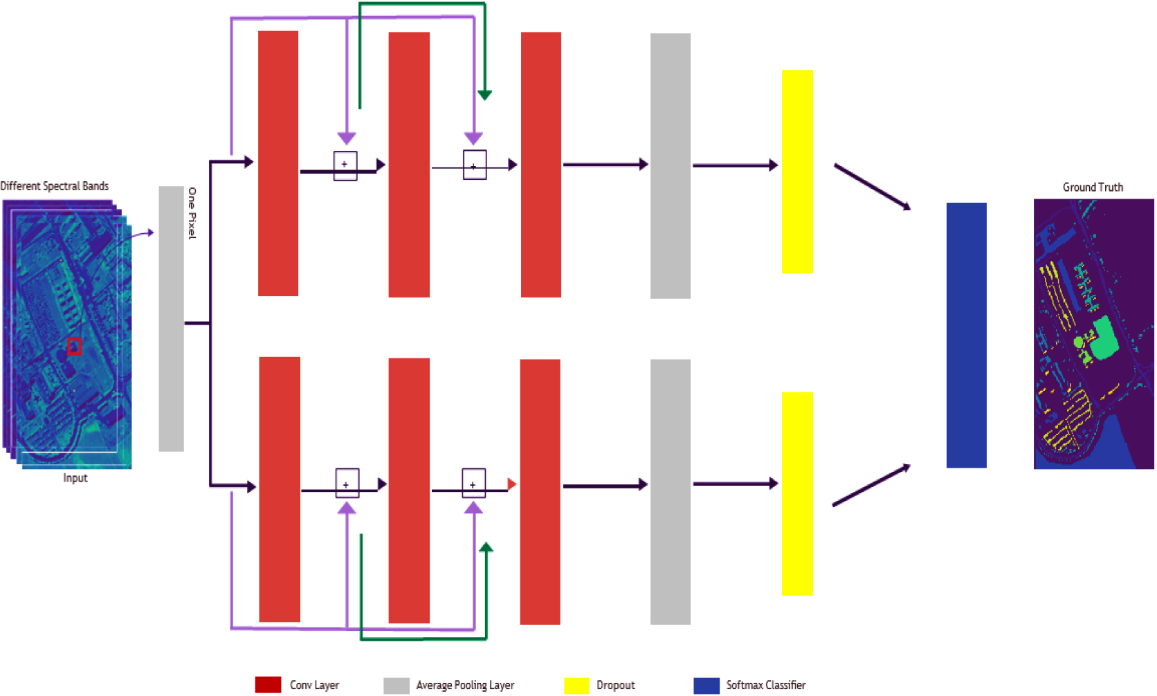

The goal of hyperspectral imaging (HSI) categorization is to categorize each pixel’s land cover according to its various frequency bands. In this study, we introduce a deep hypernetwork framework that facilitates deep HSI component development effectively without the need for additional datasets or laborious preprocessing.

Figure 2 illustrates our initial hybrid architecture, which combines elements from both ResNet and Inception networks. Two leftover blocks make up the suggested construction, as seen in Fig. 2. Three layers of convolution will be followed by a standard pooling layer. Each layer’s output is used as the input for the subsequent layer, creating a cascaded structure. Within this architecture, a single fully connected cascaded residual block is employed, where information from the layer of convolution before it is received by the subsequent layer of convolution. We found that the three layers of convolution are the best number for our model via empirical assessment.

The final pooling layer performs average pooling on the data and then passes it to the classifier. Contrarily, the convolutional layers perform operations called convolution on the supplied information. We use the Adam optimization approach (Kingma and Ba, 2014) instead of stochastic gradient descent to improve network optimization effectiveness. The Adam algorithm for optimization has benefits including computational efficacy and interference resistance.

We optimized the teaching method by setting the starting rate of learning to 0.001 and the batch size to 17 for the College of Pavia a database, Salinas a database, and Pavia Center scene database.

3.3.1 Layer 1: Convolutional

After convolution, the convolutional layers use the ReLU function to change the information. Three convolutional layers, each with nine kernels (filters), provide nine maps of features. Equation (3) explains kernel functioning.

$\displaystyle Yi=\phi\left({Zi{\ast}Yi-1+\beta i}\right)$ (3)

The $*$ in the equation represents the convolution operator, which applies the rectifier function, adds the bias term, convolves the filter $Z i$ with the input data $Yi-1$ , and produces a feature map $Y i$ .

Our suggested model comprises 16 units per layer of convolutional neural networks (1D convolution frame) and 9 layers each layer. The convolution process uses a stride length of one. We use the Glorot uniform (Xavier) value inflation approach, as advised by Glorot and Bengio (2010), for setting the weightings (kernels) of the layers of convolutional neural networks. Initial values of zero are used for biased components.

$\displaystyle\phi\left(y\right)=\textit{maximum}\left({y,0}\right)$ (4)

The ReLU activating operation, which performs an element-wise action on the given input information $y$ , is shown in Eq. (4).

Because they are better suited to the architecture of the HSI information, we decided to utilize 1D convolutional kernels rather than 2D or 3D kernels. The format of the HSI information is such that every pixel and the associated band can be saved as one vector with only one label. Our approach includes two remainder estimates that are finally coupled.

Equations (5) to (8) describes how the higher residual model works:

$\displaystyle X1=\phi\left({W1{\ast}X0+\beta 1}\right)$ (5) $\displaystyle X2=\phi\left({W2{\ast}\left({X0+X1}\right)+\beta 2}\right)$ (6) $\displaystyle X3=\phi\left({W3\ast\left({X0+X1+X2}\right)+\beta 3}\right)$ (7) $\displaystyle X4=AvgP\left({X3}\right)$ (8)

The below equations represents the formulation of the lower residual model.

$\displaystyle X^{\prime}1=\phi\left({W^{\prime}1\ast X+\beta}\right)$ (9) $\displaystyle{X}^{\prime}2=\phi(W^{\prime}2*(X^{\prime}0+X^{\prime}1)+\beta 2)$ (10) $\displaystyle X^{\prime}3=\phi\left({W^{\prime}3\ast\left({X^{\prime}0+X^{% \prime}1+X^{\prime}2}\right)+\beta 3}\right)$ (11) $\displaystyle X^{\prime}4=AvgP\left({X^{\prime}3}\right)$ (12)

Inspired by the parallelism feature of the Inception module, we incorporate it into our architecture, enabling the simultaneous operation of the top and lower residual models, which eventually merge. The first three lines in every formula describe data pooling. Following transferring the outcomes of the third layers of convolution (X3 and X03) to the average pooled level, we employ the dropout approach. Additional details on the mean pooled and dropouts methods are provided in the next section.

3.3.2 Layer 2: Pooling

Our approach uses a pooling layer for a typical pooling with a filter’s size of 2 with a stride width of 2. The typical pooled process is carried out by this layer. The average pooled functional is described in Eq. (13).

$\displaystyle Xi=AvgP\left({Xi-1}\right)$ (13)

We include an average layer of pooling which executes the average pooling procedure in our framework. This process, designated as AvgP, uses the input data $Xi-1$ from the preceding convolutional layer process as its input. It calculates the average value of the input data over a specified pooling window. After the average pooling layer, we incorporate a dropout strategy with a probability of 0.25 at the final stage. This dropout layer helps in reducing overfitting. Following the dropout layer, we employ the softmax classifier to classify the output data. The softmax classifier represents the only fully connected layer in our model.

The first level of convolution comprises 153 parameters that can be trained The second and third layer of convolutional neural networks contain 1,305 parameters to train apiece. The penultimate FC layer comprises 4,140 parameters to train for the University of Pavia database and the Pavia Central scene database. There nonetheless exist 8,109 parameters that may be trained in the Indian Pines database and 14,704 for the Salinas database. This discrepancy results from the many result classifications included in each dataset. There are nine categories of output in the University of Pavia and Pavia Centre scenario information sets, 16 in the Salinas a database, and 8 in the Indian Pines database.

In total, for the University of Pavia and Pavia Centre scene datasets, there are 8,208 trainable parameters. The Indian Pines database has 10,872 parameters that are trainable, whereas the Salinas database has 18,772. Our goal is to minimize the loss functional during training stage, as shown in Fig. 3a, in order to maximize the efficiency of the model’s parameters. The chart shows that our algorithm efficiently arrived at a regional minimum in only 50 iterations. The convergence of our model can be observed by examining the training and testing accuracies, which are presented in Fig. 3b.

4. Result

A second test dataset made up of 512 MRI scans and 112 PET images is used to evaluate the effectiveness and generalization of the suggested methods. This test a database, which is different from the source information set, makes up 60% of the total amount of information. This test database is being used to assess the model’s capacity to predict outcomes accurately for fresh information. The categories in the two collections are tiered to guarantee the same representation.

For the results presented in Table 1, the hybridized model is rigorously evaluated and assessed over 20 epochs to ensure the dependability and outcomes.

Table 1
Data obtained from 20 epochs is analyzed to examine the loss of training and techniques of test accuracy

Period	Loss of training	Accuracy of test	Period	Loss of training	Accuracy of test
1	21.8	92.6	11.0	12.2	97.1
2	21.3	93.4	12.0	11.4	97.9
3	19.2	94.5	13.0	10.6	97.9
4	18.3	94.8	14.0	9.9	98.1
5	17.3	94.9	15.0	9.1	98.1
6	16.3	95.1	16.0	7.9	98.3
7	15.8	95.7	17.0	6.9	98.4
8	14.7	95.9	18.0	6.8	98.4
9	13.6	96.8	19.0	5.9	98.4
10	13.1	96.9	20.0	5.7	98.5

Figure 3.

Showcases the progression of our model’s performance during the convergence phase. Subfigure (a) displays the changes in the loss function, indicating how it is minimized over time. In subfigure (b), the corresponding accuracy values for both training and testing data are depicted, illustrating the model’s improvement as it converges.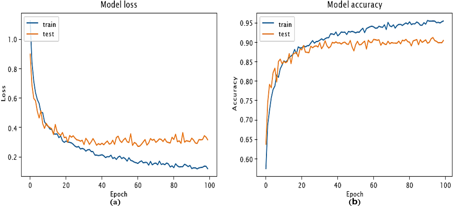

The proposed model achieves a high level of accuracy on the test dataset, with a standard accuracy of 92.8% and 98.5%. With a median range from 0.80 to 0.83 for the ROC & AUC the model operates even better. Figure 4’s boxplots show that conversion and risk classification have equivalent correctness and ROC. In comparison to risk, the specific conversions ratios vary from 7.6% to 92.76%.

In terms of identifying patients with progressing mild cognitive impairment (pMCI) and estimating the time to admission, the model outperforms random categorization. The combined model is 19.8% more accurate than probability in discriminating pMCI from stabilized MCI (sMCI). Furthermore, the model more reliably places patients with pMCI in the category with the shortest duration to treatment by 33.89% when contrasted with random error. The goal of this project is to create a hybrid CNN system that can tell people with moderate cognitive decline and AD apart from those who are steady. The suggested model also takes taken into consideration how long it generally takes for AD to develop by putting people into various categories of risk depending on whether they are likely to develop AD inside 24 months (high risk), outside 24 months (low risk), or not at all (sMCI).

The baseline measurements used in this study are obtained from the initial visit of each individual, providing an accurate representation of their initial healthcare encounter.

Figure 4.

AD diagnosis using pre-imaging database values.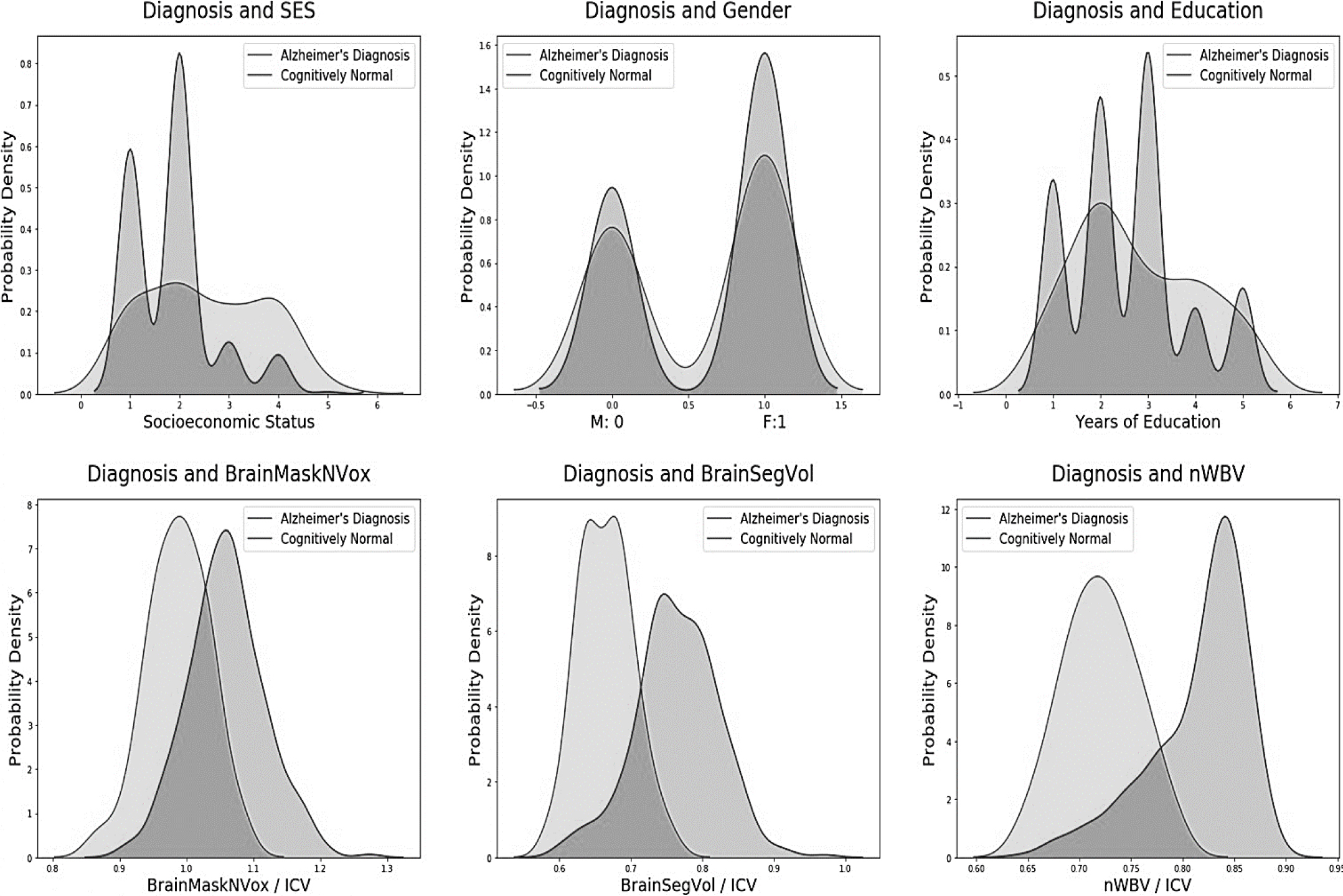

The suggested hybrid model includes a number of cutting-edge, outstanding durability methods. Recent developments in preprocessing and ML techniques, especially for early AD forecasting investigation, are covered in a literature analysis that was undertaken. Many existing approaches for pMCI & sMCI include MRI image analysis as part of their preprocessing pipeline. Furthermore, the successful results achieved, with cross-validation accuracy and area under the curve (AUC) above 80%, can be attributed to domain learning. Domain acquisition entails the extraction of useful auxiliary traits from a related area, such as the classification of AD patients vs intellectually healthy people. Each study that makes use of domain expertise raises the validity of the results.

Table 2

Performance comparison

Techniques	Accuracy in %	Precisionin %	Recallin %
PCA with NN	94.90	90.90	97.90
3D $+$ CNN	92.90	93.08	89.90
Resnet18s	98.78	99.00	99.79
LSTMs	79.62	69.86	59.56
CNNs	91.90	90.90	92.90
Hybrid (CNN $+$ Resnet18)	98.40	94.70	97.90

Figure 5.

MRI image categorization results reveal classification 0 as no Alzheimer’s disease and classification 1 as an Alzheimer-afflicted brain.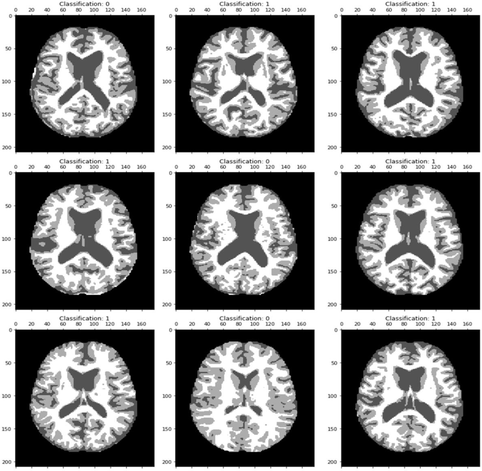

Figure 6.

ROC curve with 0.82 TPR & FPR.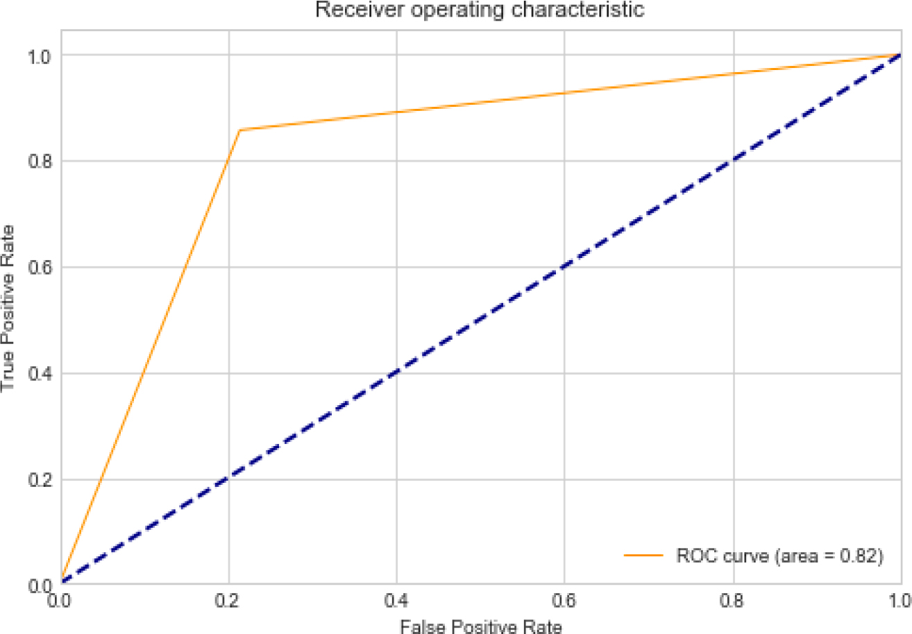

Figure 7.

A first 20 epochs’ validation and training loss reveal a constant difference, pointing to a well-fitted curve.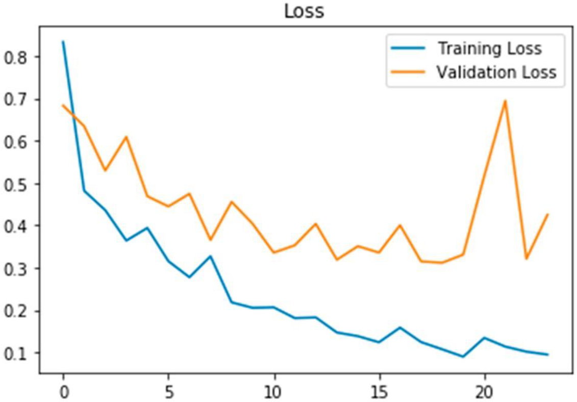

Figure 8.

A good fit model is demonstrated by both the training and validation accuracy values having the smallest difference between them.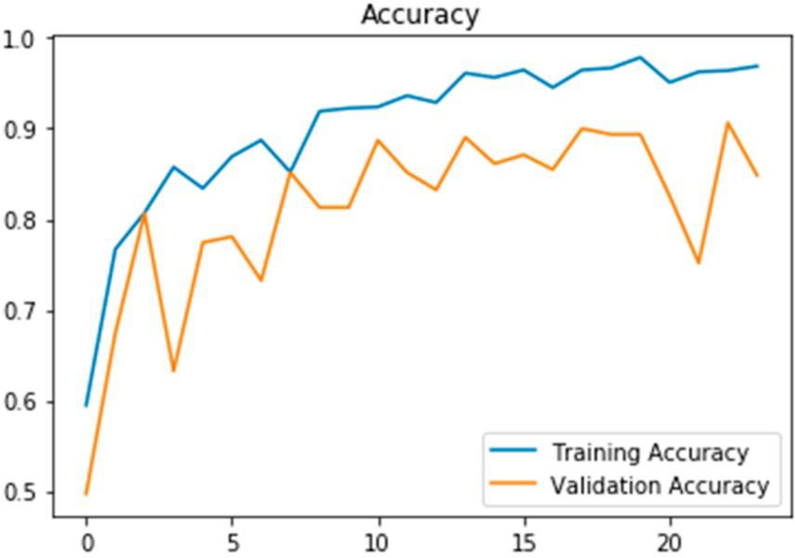

Figure 9.

Performance comparison of proposed model.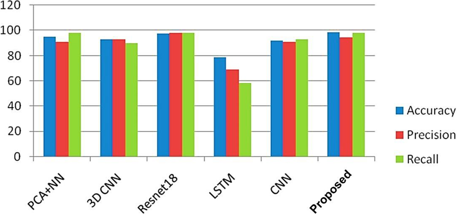

Figure 5 presents the findings of the MRI image classification, where dementia is categorized in specific locations within the images. The link between the TPR & FPR is shown by the ROC curve, which is shown in Fig. 6. It offers a graphic depiction of how well the suggested approach performs in differentiating between events that are positive or negative. With the help of Fig. 7, which shows the loss of training & validity over the course of 20 epochs, it is possible to assess how the model is progressing in its learning process and how well it can generalize to new data. The model’s performance on the training and validation datasets is demonstrated in Fig. 8 by the training and validation accuracy after 20 iterations, which demonstrates how well the model works over time. The performance of various techniques, such as PCA, CNN, Resnet18, and DCNN, has been compared to the proposed model. The comparison results are presented in Fig. 9, which provides a visual representation of the performance metrics.

The creation of a mixture of models effectively satisfies the paper’s goals since it can detect the change from stability to progressive MCI and make better forecasts about how long AD will continue for. The outcomes of Multi-validation DL, however, emphasize the necessity for more work on the framework of the model and hyperparameter optimization techniques. Given the restricted information and requirements, enhancing the extraction of features and performance involves altering these processes. In a field with little information, obtaining the best possible use of it is vital.

Domain learning has shown promise in enhancing model performance, as evidenced by the number of publications employing this strategy. While training the model’s weights to detect auxiliary AD categories alongside non-AD categories may not immediately improve efficiency on the core issue, it could accelerate resolution and minimize training time. Brain partitioning is an additional tactic that may be used to enhance efficiency. More accurate data may be gleaned from certain brain regions (temporal, parietal, prefrontal, and occipital) utilizing parallel 3-D convolutional layers of data, thereby condensing the complicated structure of features. This approach could simplify the identification of valuable features within a smaller feature area.

5. Conclusion

In summary, the goal of this research was to increase the precision of AD predictions using a hybrid model that combines CNNs and denoising methods with a MLP. We evaluated the effectiveness of our suggested model in comparison to a number of different techniques, such as PCA with NN, 3D $+$ CNN, Resnet18, LSTM, and CNN. The results of the study show how well our mixed approach performs in terms of properly forecasting AD. The hybrid model achieved an impressive accuracy of 98.40% on the test dataset, outperforming other methods such as PCA with NN (94.90%), 3D $+$ CNN (92.90%), Resnet18 (97.78%), LSTM (78.62%), and CNN (91.90%). The incorporation of both deep CNN and denoising MLP techniques in our hybrid model contributed to its superior performance. The deep CNN component enabled the extraction of high-level features from the input data, while the denoising MLP helped to reduce noise and enhance the quality of the input data, leading to improved prediction accuracy. Moreover, the combination of CNN and Resnet18 architectures in our hybrid model further enhanced the predictive power. The Resnet18 component provided a deeper network with residual connections, allowing for better learning and representation of complex patterns in the data. Our research shows how crucial it is to use mixed algorithms and take advantage of the advantages of various deep learning approaches when attempting to anticipate the onset of AD. Our hybrid algorithm’s outstanding precision indicates that it has the potential to be an important tool for the early identification and identification of AD, that may have a big influence on the management of patients and their results.

In future study, greater and more varied information could potentially be used to test the blended model’s generalization and resilience. Additionally, fine-tuning and optimization of the model’s hyperparameters could be explored to further improve its performance.

References

Alzheimer’s Association. 2018 Alzheimer’s disease facts and figures. Alzheimer’s Dement. 2018; 14: 367-429.

Korolev

. Alzheimer’s disease: A clinical and basic science review. Med. Stud. Res. J. 2014; 4: 24-33.

Kulurkar

Kumar Dixit

Bharathi

Monikavishnuvarthini

Dhakne

Preethi

. AI based elderly fall prediction system using wearable sensors: A smart home-care technology with IOT. Measurement: Sensors. 2023; 25: 100614.

Moon

Lee

Choi

. Changes in the hippocampal volume and shape in early-onset mild cognitive impairment. Psychiatry Investig. 2018; 15: 531.

Bai

Preethi

. Security Enhancement of Health Information Exchange Based on Cloud Computing System. International Journal of Scientific Engineering and Research. 2016; 4(10): 79-82.

Hazarika

Maji

Sur

Paul

Kandar

. A Survey on Classification Algorithms of Brain Images in Alzheimer’sDisease Based on Feature Extraction Techniques. IEEE Access. 2021; 9: 58503-58536.

NIH. Alzheimer’s Disease: A Clinical and Basic Science Review. Available online: https://www.nia.nih.gov/health/alzheimersdisease-fact-sheet (accessed on 13 July 2020).

Alzheimer’s Association. Alzheimer’s Disease Fact Sheet. Available online: https://www.alz.org/in/dementia-alzheimers-en.diagnosis (accessed on 13 July 2020).

Preethi

Asokan

. Neural network oriented roni prediction for embedding process with hex code encryption in dicom images. In Proceedings of the 2nd International Conference on Advances in Computing, Communication Control and Networking (ICACCCN), Greater Noida, India (2020 December), (pp. 18-19).

10.

National Institute on Aging(NIH). What Is Mild Cognitive Impairment? Available online: https://www.nia.nih.gov/health/what-mild-cognitive-impairment (accessed on 23 June 2021).

11.

Preethi

Asokan

Thillaiarasu

Saravanan

. An effective digit recognition model using enhanced convolutional neural network based chaotic grey wolf optimization. Journal of Intelligent & Fuzzy Systems. 2021; 41(2): 3727-3737.

12.

Mayo Clinic Staff. Learn How Alzheimer’s Is Diagnosed. 2019. Available online: https//www.mayoclinic.org/diseasesconditions/alzheimers-disease/in-depth/alzheimers/art-20048075: (accessed on 23 June 2021).

13.

Huff

Boller

Lucchelli

Querriera

Beyer

Belle

. The neurologic examination in patients with probable Alzheimer’sdisease. Arch. Neurol. 1987; 44: 929-932.

14.

Arevalo-Rodriguez

Smailagic

Figuls

Ciapponi

Sanchez-Perez

Giannakou

Pedraza

Cosp

Cullum

. Mini-Mental State Examination (MMSE) for the detection of Alzheimer’s disease and other dementias in people withmild cognitive impairment (MCI). Cochrane Database Syst. Rev. 2015; 23: 107-120.

15.

Cummings

Ross

Absher

Gornbein

Hadjiaghai

. Depressive symptoms in Alzheimer disease: Assessment anddeterminants. Alzheimer Dis. Assoc. Disord. 1995; 9: 87-93. [PubMed]

16.

Symms

Jäger

Schmierer

Yousry

. A review of structural magnetic resonance neuroimaging. J. Neurol. Neurosurg. Psychiatry. 2004; 75: 1235-1244. [PubMed]

17.

Ijaz

Attique

Son

. Data-driven cervical cancer prediction model with outlier detection and over-sampling methods. Sensors. 2020; 20: 2809.

18.

Ledig

Schuh

Guerrero

Heckemann

Rueckert

. Structural brain imaging in Alzheimer’s disease and mildcognitive impairment: Biomarker analysis and shared morphometry database. Sci. Rep. 2018; 8: 1-16.

19.

Fung

Guan

Kumar

Fiterau

. Alzheimer’s disease brain mri classification: Challenges and insights. arXiv2019, arXiv1906.04231.

20.

Mirzaei

Adeli

. Machine learning techniques for diagnosis of alzheimer disease, mild cognitive disorder, and other types ofdementia. Biomed. Signal Process. Control. 2022; 72: 103293.

21.

Islam

Zhang

. A novel deep learning based multi-class classification method for Alzheimer’s disease detection usingbrain MRI data. In Proceedings of the International Conference on Brain Informatics; Springer: Berlin/Heidelberg, Germany, 2017; pp. 213-222.

22.

Zhang

Wang

Zhang

. Multi-modal deep learning model for auxiliary diagnosis of Alzheimer’sdisease. Neurocomputing. 2019; 361: 185-195.

23.

Shanmugam

Duraisamy

Simon

Bhaskaran

. Alzheimer’s disease classification using pre-trained deep networksBiomed. Signal Process. Control. 2022; 71: 103217.

24.

Kong

Zhang

Zhu

Wang

Zhang

. Multi-modal data Alzheimer’s disease detection based on 3D convolution. Biomed. Signal Process. Control. 2022; 75: 103565.

25.

Orouskhani

Rostamian

Zadeh

Shafiei

Orouskhani

. Alzheimer’s Disease Detection from Structural MRI UsingConditional Deep Triplet Network. Neurosci. Inform. 2022; 100066.

26.

Sharma

Lakhotia

Sain

Brahmachari

. Early prediction and monitoring of sepsis using sequential long short term memory model. Expert Systems. 2021; 39: 101111/exsy.12798.

27.

Datta Gupta

Sharma

Ahmed

. et al. A Novel Lightweight Deep Learning-Based Histopathological Image Classification Model for IoMT. Neural Process Lett. 2023; 55: 205-228. doi: 10.1007/s11063-021-10555-1.

Development of hybrid deep CNN with denoising MLP for accurate prediction of Alzheimer’s disease

Abstract

Keywords

1. Introduction

3. Proposed methodology for AD prediction

3.1 Preprocessing of data using MLP

3.2.2 Loss of function

Table 1 Data obtained from 20 epochs is analyzed to examine the loss of training and techniques of test accuracy

References

Table 1
Data obtained from 20 epochs is analyzed to examine the loss of training and techniques of test accuracy