
Abstract
School value-added models are widely applied to study, monitor, and hold schools to account for school differences in student learning. The traditional model is a mixed-effects linear regression of student current achievement on student prior achievement, background characteristics, and a school random intercept effect. The latter is referred to as the school value-added score and measures the mean student covariate-adjusted achievement in each school. In this article, we argue that further insights may be gained by additionally studying the variance in this quantity in each school. These include the ability to identify both individual schools and school types that exhibit unusually high or low variability in student achievement, even after accounting for differences in student intakes. We explore and illustrate how this can be done via fitting mixed-effects location scale versions of the traditional school value-added model. We discuss the implications of our work for research and school accountability systems.
Keywords
1. Introduction
School value-added models attempt to estimate school differences in student achievement and are widely applied in educational (Goldstein, 1997; Reynolds et al., 2014; Teddlie & Reynolds, 2000) and statistical research (American Statistical Association, 2014; Braun & Wainer, 2007; McCaffrey et al., 2004; Raudenbush & Willms, 1995; Wainer, 2004). They are also used in the United States, United Kingdom, and other school accountability systems, where the predicted school differences, often referred to as school value-added scores, provide the basis of reward and sanction decisions on schools (Amrein-Beardsley, 2014; Castellano & Ho, 2013; Koretz, 2017; Leckie & Goldstein, 2017; Organization for Economic Cooperation and Development, 2008). In educational and statistical research, there is an additional interest in identifying school policies and practices that predict the school differences and that might therefore prove effective at raising student achievement in schools in general.
The traditional school value-added model is formulated as a mixed-effects (multilevel or hierarchical) linear regression model (Goldstein, 2011; Raudenbush & Bryk, 2002; Snijders & Bosker, 2012) of student current achievement on student prior achievement measured at the start of the value-added period (typically defined as one or more school years or a phase of schooling) and a school random intercept effect to predict the school differences (Aitkin & Longford, 1986; Goldstein et al., 1993; Raudenbush & Bryk, 1986). The adjustment for student prior achievement is fundamental as simpler comparisons of unadjusted school mean achievement would in large part reflect school differences in student achievement present at the start of the value-added period. Such differences are argued beyond the control of the school. Student sociodemographic characteristics are often added to adjust for initial school differences in student composition more convincingly (Ballou et al., 2004; Leckie & Goldstein, 2019; Leckie & Prior, 2022; Levy et al., 2023). Schools with higher scores are described as adding more value: producing higher student achievement for any given set of students. The scores are argued to reflect the net influences of differences in the quality of teaching, availability of resources, and other policies and practices across schools, which are typically unobserved to the data analyst. The regression coefficient on student prior achievement is occasionally allowed to vary across schools. The resulting random slope model is sometimes referred to as a “differential school effectiveness” model as this extension allows schools to now have different effects for different types of students (Nuttal et al., 1989; Scherer & Nilsen, 2019; Strand, 2010).
While the traditional school value-added model is widely applied (Levy et al., 2019), it is important to realize that this model is just a regression model fitted to observational data and so the effects attributed to schools may also be caused by other factors that are not captured by the model (American Statistical Association, 2014). That is, while there is consensus that the predicted school effects are fairer and more meaningful measures to compare schools than comparing simple school mean achievement scores, the additional assumptions required to interpret these predicted school effects as causal effects rather than as merely adjusted school mean differences are challenging (Amrein-Beardsley, 2019; Reardon & Raudenbush, 2009; Rubin et al., 2004). For example, the school-level exogeneity assumption (independence of covariates and school random effect) will fail if higher prior achieving students select into more effective schools, perhaps because such students are from more affluent families who are more able to buy into the catchment areas of these schools (Angrist et al., 2021; De Fraine, 2002; Thomas & Mortimore, 1996; Timmermans & Thomas, 2015). The parameter estimates of the school value-added models presented in this article should therefore be viewed as the measures of association and the predicted school effects as descriptive differences in means and variances of student achievement across schools, where inevitably only partial and imperfect adjustments have been made for school differences in student characteristics at intake.
In the traditional school value-added model, the difference between observed and predicted student current achievement defines the total residual, which can be viewed as a covariate-adjusted (residualized) measure of student current achievement (i.e., a controlled comparison of student achievement levels). The total residual is modeled as the summation of the school random intercept effect and the student residual. The school random effect measures the mean student adjusted achievement in each school. In contrast, the constant residual variance implicitly assumes the variance in student adjusted achievement is the same in every school. This inconsistent modeling of the mean and variance does not seem realistic. Any given school policy or practice will have different effects on students as a function of their observed and unobserved characteristics and will therefore contribute to the variance in student adjusted achievement operating in each school. Indeed, this is the motivation for the random slope extension to the traditional value-added model described above. In practice, however, this extension can only be used to account for a limited number of observed student characteristics, not to all observed and unobserved student characteristics (Raudenbush & Bryk, 2002). Thus, the different sets of school policies and practices operating in each school will lead the variance in student adjusted achievement to vary across schools, even in random slope models.
Studying the variance in student adjusted achievement in each school may therefore provide valuable new insights into the differences in student learning between schools. Consider two schools that show similarly high levels of mean student adjusted achievement. The traditional school value-added model would describe these two schools as equally effective. Suppose, however, the first school shows higher variance in their student adjusted achievement scores than the second school. Which school should now be viewed more positively? The school with the higher variance will have more students making exceptionally high adjusted achievement (a positive) albeit at the expense of more students also making unacceptably low adjusted achievement (a negative). All else equal, the school with the higher variance will also show a weaker link between prior and current achievement, and so in this school, low prior achievement students are more able to raise up the achievement distribution (a positive), but equally and necessarily, high prior achievement students are more likely to fall down the distribution (a negative). Thus, in part, how higher variance should be viewed depends on value judgements regarding whether such positives outweigh such negatives. These are not simple questions to answer. Also relevant is the underlying explanation for the difference in variance. For example, if the higher variance seen in the first school is a result of its school policies and practices having greater differential effects on different student groups versus the second school, then higher variance might be viewed as a negative as the explanation implies that the school might not be in sufficient control in the implementation of its policies and practices and is exacerbating inequities in student learning versus the first school (Nuttal et al., 1989; Scherer & Nilsen, 2019; Strand, 2010). Though, here too, a tension lies around what is the optimal level of control. Again, these are not simple questions to answer. More generally, school differences in the adjusted variances, just like school differences in the adjusted means, may also reflect unmodeled school differences in student intake, and so, it is important to attempt to adjust fully for such differences.
A necessary first step to addressing these bigger questions and debates is to first measure school differences in the variance in student adjusted achievement. Only then can school effectiveness and other researchers follow up individual schools, which show unusually high or low variance to try to identify the specific school policies and practices, which are associated with this. Similarly, only then, can school accountability systems, via school inspections, ask schools to reflect on any unusual school variance scores and discuss these within the broader context of what is happening in these schools and other schools facing similar challenges. All these discussions should be alert to the descriptive rather than causal nature of the statistics and to the limitations of the data more generally, and these statistics should not be used to make automatic high-stakes judgements on schools.
The aim of this article is to therefore broaden the traditional school value-added model to study the effects of schools on not just mean student current achievement, but the variance in student current achievement. We do this by applying mixed-effect location scale (MELS) models to student current achievement. MELS models are an extension to conventional mixed-effects linear regression models that model the residual variance not as a constant, but as a function of the covariates and a new random effect. Thus, the residual variance is now allowed to vary across the schools. Hedeker et al. (2008) illustrated the MELS model in the context of studying intensive longitudinal data on mood. Subsequently, Hedeker and others further developed this class of models and applied it to a range of other longitudinal psychological and health data (e.g., Goldstein et al., 2018; Hedeker et al., 2012; Nordgren et al., 2020; Parker et al., 2021; Rast et al., 2012). Just as mixed-effects models more generally are routinely also applied to clustered cross-sectional data, so can MELS models. Indeed, several such applications have now been published, including in social science research (Brunton-Smith et al., 2017, 2018; Leckie et al., 2014; McNeish, 2021). However, the applicability of MELS models to school value-added studies has not yet been explored. We address this via an application to school value-added models for school accountability in London, England. Specifically, we examine the following research question: How does the variance in student adjusted achievement vary across schools?
This article proceeds as follows. In Section 2, we introduce our application. In Section 3, we present the traditional random-intercept and -slope linear regression school value-added models and their extensions to MELS models. In Section 4, we present the results. In Section 5, we provide a general discussion, including implications of our work for research and school accountability.
2. Application
Background
In England, since 2004, the Government has published school value-added scores derived from school value-added models for all secondary schools in the country in annual school performance tables (https://www.gov.uk/school-performance-tables). These scores aim to measure the value that each school adds to student achievement between the end of primary schooling national Key Stage 2 (KS2) tests (age 11, academic year 6) and the end of compulsory secondary schooling General Certificate of Secondary Education (GCSE) examinations (age 16, academic year 11). The scores play a pivotal role in the national school accountability system, informing school inspections and judgments on schools. They are also promoted to parents as a source of information when choosing schools for their children. Their high stakes use and public presentation have drawn sustained criticism from the academic literature (Goldstein & Spiegelhalter, 1996; Leckie & Goldstein, 2009, 2017, 2019; Prior, Jerrim, et al., 2021). Nevertheless, these authors also argue that when used carefully and collaboratively with schools in a sensitive and less public manner, there is still an important role for these scores to help identify and understand differences in student outcomes across schools, and it is in this spirit that we have carried out the current research (Goldstein, 2020).
Data, Sample, and Variables
We focus on schools in London and on those students who took their GCSE examinations in 2018 and therefore KS2 tests in 2013. The sample is drawn from the National Pupil Database (Department for Education [DfE], 2023) a census of all students in state education and consists of 71,321 students in 465 schools (mean = 153 students per school, range = 14–330).
Student current and prior achievement are measured by students’ GCSE examination and KS2 test scores (DfE, 2020). We standardize these scores to have means of 0 and standard deviations (SDs) of 1, so that the measures can be interpreted in SD units. Henceforth, we refer to these standardized scores simply as the student age 16 and 11 scores. Figure 1 shows both scores are approximately normally distributed and linearly related with a strong Pearson correlation of 0.72. There are very slight floor and ceiling effects in age 16 scores.
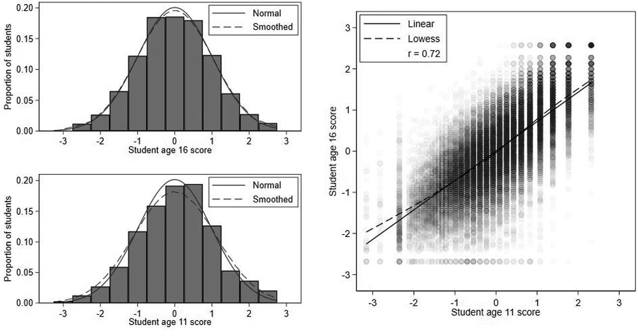
Histograms and scatterplot of student age 16 and age 11 scores.
Table 1 presents the summary statistics for the student characteristics. Of note, 61% of students are non-White and 35% poor (as measured by receipt of free school meals [FSMs]). The London sample is therefore more ethnically diverse and poorer than the full English sample, where only around 25% of students are non-White and 25% poor (Leckie & Goldstein, 2019).
Summary Statistics for the Student Characteristics
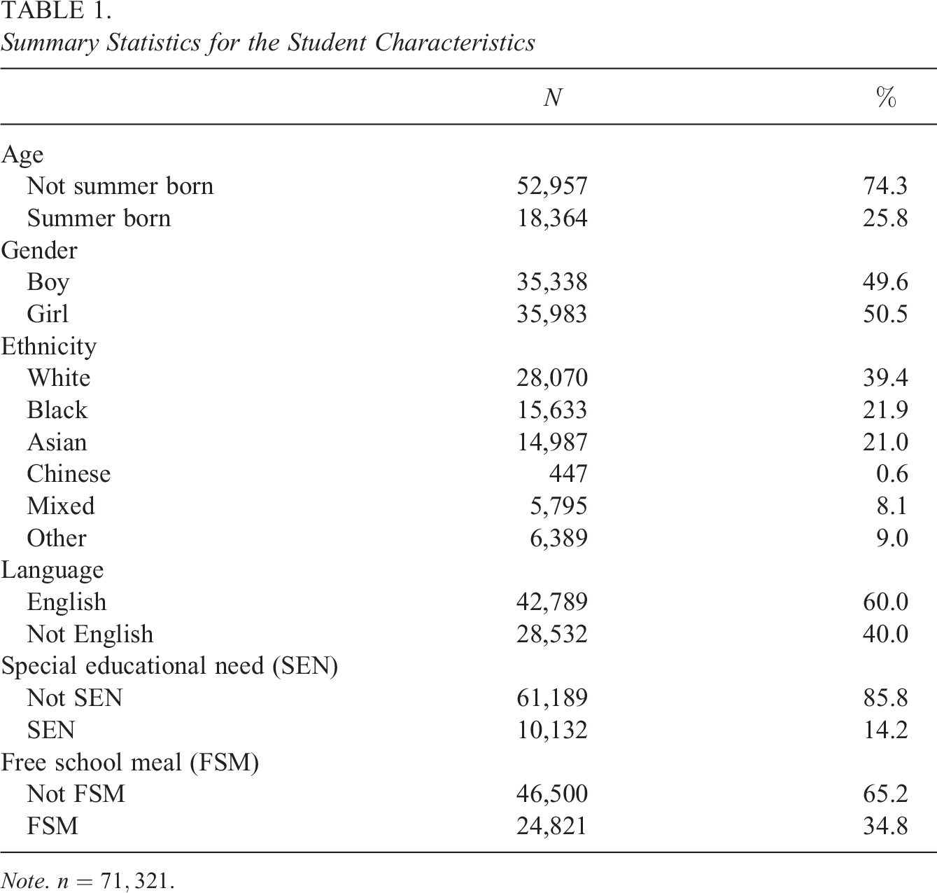
Note.
Table 2 presents the summary statistics for the school characteristics. A range of school types operate in London (Leckie & Goldstein, 2019), and we have categorized these into four groups: standard, sponsored academy, converter academy, and other. Standard school type encompasses community, foundation, voluntary aided, voluntary controlled, and city technology colleges. In contrast to standard and other schools, academies receive their funding directly from the government rather than through local authorities (school districts). Sponsored academies are mostly underperforming schools, which have been required to change to academy status and are run by sponsors. Converter academies are successfully performing schools that have opted to convert to academy status. Other school type encompasses free, studio, university technology colleges (UTCS), and further education colleges. These are more technically or vocationally oriented schools.
A minority of local authorities operate selective rather than comprehensive admissions. In these areas, grammar schools select students based on high performance in entrance examinations and so by definition have high mean age 11 scores and tend also to be educationally advantaged and homogenous in terms of student sociodemographic characteristics. Secondary modern schools take those students not admitted to grammar schools.
Summary Statistics for the School Characteristics
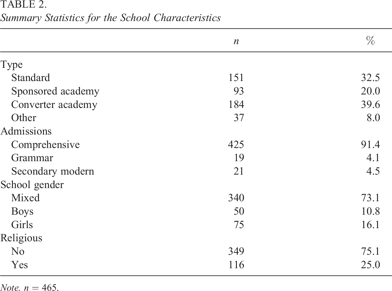
Note.
3. Models
Model 1: Random-Intercept Model
The traditional school value-added model (Aitkin & Longford, 1986; Goldstein et al., 1993; Raudenbush & Bryk, 1986) can be written as the following random-intercept linear regression:
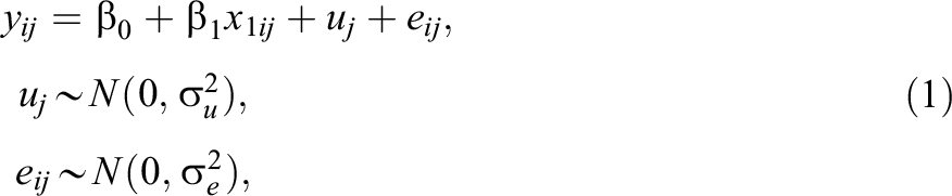
where
The total residual
Figure 2 illustrates the main details of this and subsequent models using hypothetical data on two schools. In each case,
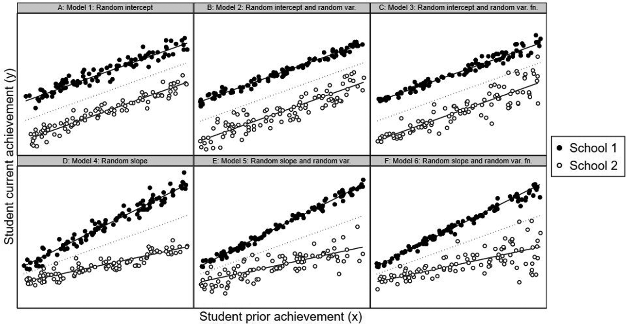
Illustration of different models using hypothetical student current and prior achievement scores data for two schools, School 1 (solid markers) and School 2 (hollow markers). Panel A: Random-intercept model. Panel B: Random-intercept model with random residual variance. Panel C: Random-intercept model with random residual variance function. Panel D: Random-slope model. Panel E: Random-slope model with random residual variance. Panel F: Random-slope model with random residual variance function.
Model 2: Random-Intercept Model With Random Residual Variance
Model 2 extends Model 1 by allowing the variance in student adjusted achievement
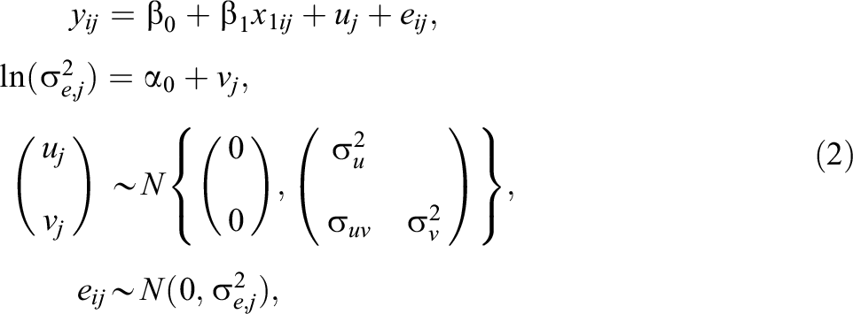
where the second line of the equation specifies the residual variance
Model 3: Random-Intercept Model With Random Residual Variance Function
Recall the reason for entering student prior achievement (and potentially further student covariates) into the mean function of the model is that schools should not be held accountable for pre-existing differences in student achievement across schools at the start of the value-added period (Ballou et al., 2004; Leckie & Goldstein, 2019; Leckie & Prior, 2022; Levy et al., 2023). A similar argument applies when comparing the variance in student adjusted achievement across schools. For example, suppose the residual variance increases with increasing student prior achievement. This would suggest that schools with higher mean student prior achievement would in general be expected to show more variable student adjusted achievement than schools with lower mean student prior achievement and this is even though we have adjusted for student prior achievement in the mean function. However, following the arguments underpinning the traditional value-added model, this should be viewed as a reflection of their school intake rather than reflecting their school policies and practices. By entering student prior achievement into the model for the variance, we adjust for this overall variance trend. Focus then shifts to how schools deviate from this overall trend.
Model 3 therefore extends Model 2 by adding student prior achievement to the residual variance function. The model is written as
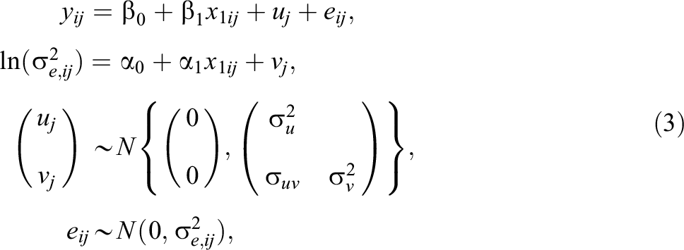
where
Model 4: Random-Slope Model
Model 4 is the differential effects version (Nuttal et al., 1989; Scherer & Nilsen, 2019; Strand, 2010) of the traditional school value-added model (Model 1) and can be written as the following random-slope linear regression:
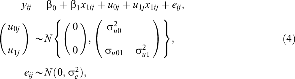
where
The total residual, now
Figure 2D illustrates Model 4, where
School mean student adjusted achievement, averaging over all students in each school, is given by
Model 5: Random-Slope Model With Random Residual Variance
Model 5 extends Model 4 by allowing the variance in student adjusted achievement to vary across schools. (Equally Model 5 extends Model 2 by adding a random slope in the mean function to student prior achievement.) We do this by specifying an MELS version of the previous model. The model can be written as
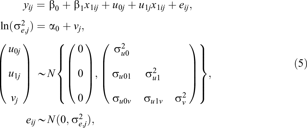
where the second line of the equation specifies the log-linear function for the residual variance (see also Model 2). The three random effects
School mean student adjusted achievement (averaging over all students) is then given by
Model 6: Random-Slope Model With Random Residual Variance Function
Model 6 extends Model 5 by adding student prior achievement to the residual variance function. (Equally Model 6 extends Model 3 by adding a random slope to student prior achievement.) The model is written as
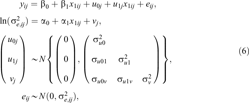
where
As in Model 5 (and Model 4), school mean student adjusted achievement (averaging over all students) is once again given by
Software
The traditional school value-added models (Models 1 and 4) are typically fitted via maximum likelihood estimation using conventional mixed-effects linear regression routines in standard software (R, SAS, SPSS, and Stata). However, the MELS versions of these models (Models 2, 3, 5, and 6) cannot be fitted using these routines, nor can they be fitted in specialized mixed-effects modeling packages (HLM and MLwiN). Hedeker and colleagues have developed the MixWILD software to fit MELS models by maximum likelihood estimation (Dzubur et al., 2020). These models can also be fitted via Markov Chain Monte Carlo (MCMC) methods in Stata and Mplus (McNeish, 2021), as well as dedicated Bayesian software such as Stan (including via the brms package in R; e.g., Parker et al., 2021), WinBUGS, OpenBUGS, and JAGS (including via the R2jags package R: e.g., Barrett et al., 2019). To support readers wishing to implement these models, we present annotated MixWILD, R, and Stata instructions and syntax and simulated data (Section S4 of the Supplemental information).
We fit all models using Stata (StataCorp, 2021). Specifically, we use the bayesmh command, which implements an adaptive Metropolis–Hastings MCMC algorithm. We use hierarchical centering reparameterizations to improve mixing. We specify vague (diffuse) normal priors for all regression coefficients and minimally informative inverse Wishart priors for the random effects variance–covariance matrices. We specify overdispersed initial values for all parameters. We fit all models with four chains, each with 5,000 burnin iterations and 10,000 monitoring iterations. We judge convergence using Gelman–Rubin convergence diagnostics (Gelman & Rubin, 1992) and trace, autocorrelation, and scatter plots. All models converged and all parameters had effective sample sizes > 400. We compare model fit using the deviance information criterion (DIC; Spiegelhalter et al., 2002). Smaller values are preferred.
4. Results
Model 1: Random-Intercept Model
Model 1 (Equation 1) is the traditional school value-added model. In other words, the random-intercept model. For simplicity and because not all researchers wish to additionally include student sociodemographics (Leckie & Prior, 2022; Levy et al., 2023), we only adjust for student prior achievement in this and subsequent Models 1 through 6, but we do explore the role of further covariates in Models 7 and 8. For the purpose of comparing to subsequent models, we parameterize
Table 3 presents the results. The estimated slope coefficient on student age 11 score is
Results for the Random-Intercept Models Adjusting Only for Student Prior Achievement
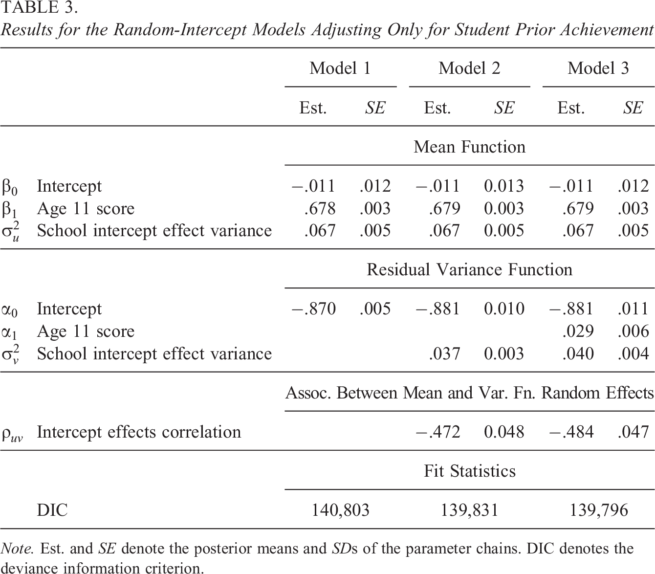
Note. Est. and SE denote the posterior means and SDs of the parameter chains. DIC denotes the deviance information criterion.
Model 2: Random-Intercept Model With Random Residual Variance
Model 2 (Equation 2) extends the random-intercept model (Model 1, Equation 1) to allow the residual variance and therefore variance in student adjusted achievement to vary across schools. Model 2 shows a reduction in the DIC of 972 points, confirming that this variation in variances is statistically significant. The mean function parameter estimates are largely unchanged. The estimated residual variance function intercept and estimated variance of the new school random effect are
Figure 3 plots the predicted school means of student adjusted achievement uj
(y-axis) against the predicted school variances
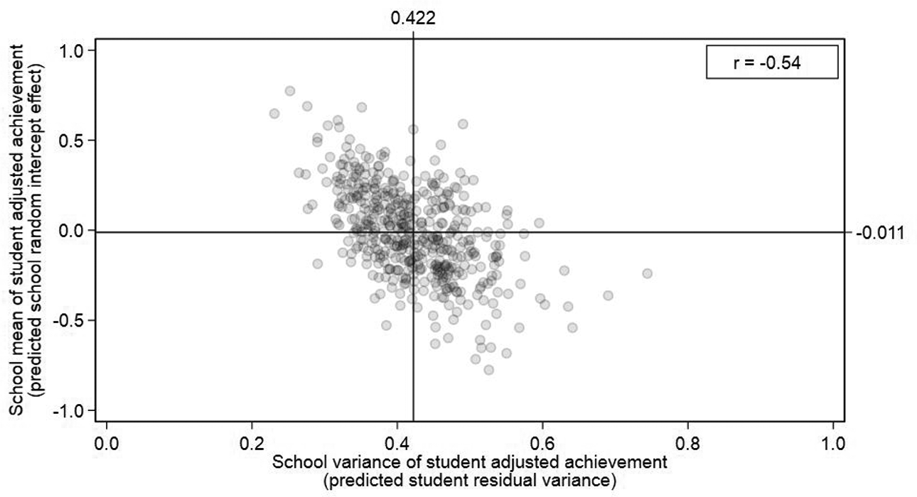
Model 2 scatterplot of school means against school variances of student adjusted achievement. London average values are shown by horizontal and vertical reference lines.
Figure 4 presents the “caterpillar plots” of the 465 predicted school means (left panel) and school variances (right panel; Goldstein, 2011). Such plots are routinely used by researchers and accountability systems to identify schools that are significantly different from average (e.g., Prior et al., 2021). The distribution of the school variances is positively skewed, consistent with being modeled as log-normally distributed. Schools with fewer students have wider 95% credible intervals than schools with more students. Only 117 of the 465 schools (25%) can be statistically separated from the overall average in terms of their school variances compared to 320 schools (69%) when we consider the school means.
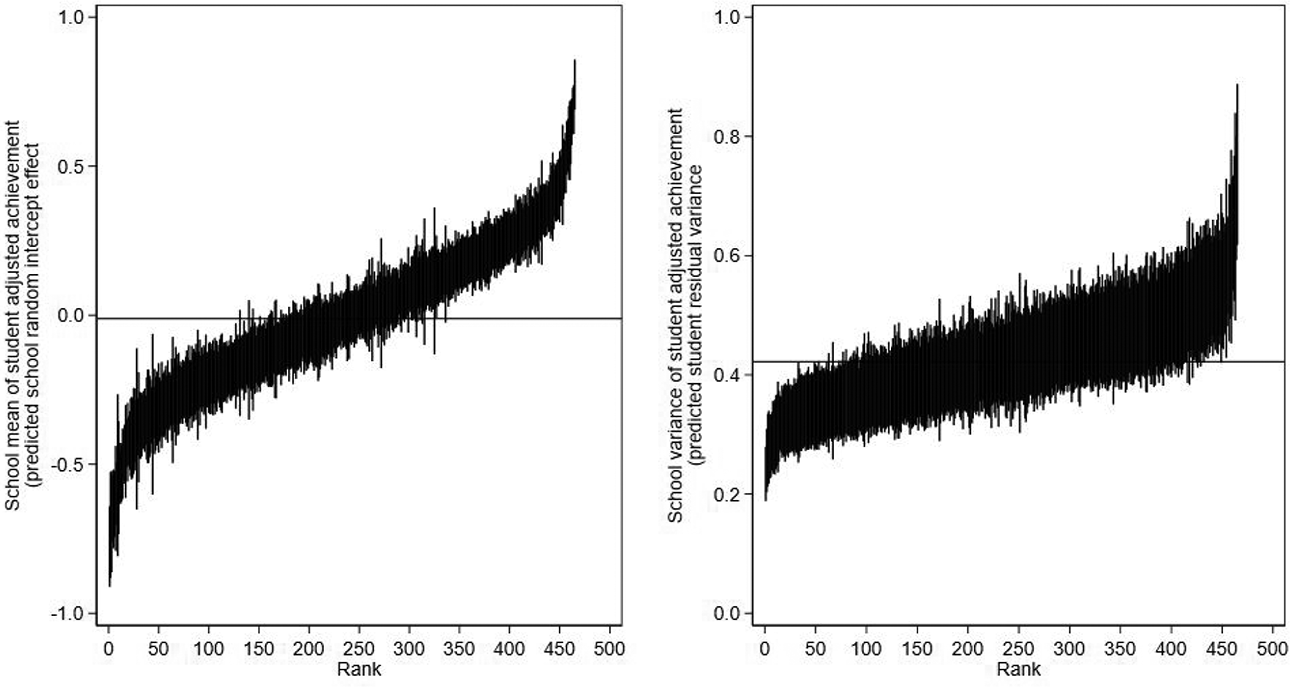
Model 2 caterpillar plots for school means (left) and school variances (right) of student adjusted achievement presented in rank order. Posterior means with 95% credible intervals.
Model 3: Random Intercept Model With Random Residual Variance Function
Model 3 (Equation 3) further extends the random-intercept model to allow the residual variance to vary not just across schools (Model 2, Equation 2), but additionally as a function of student prior achievement. Model 3 is preferred to Model 2 (Δ
Model 4: Random-Slope Model
Model 4 (Equation 4) is the differential effectiveness version of the traditional school-value-added model. In other words, the random-slopes model. Recall that this model, like the traditional random-intercepts model (Model 1, Equation 1), assumes the residual variance is once again constant across all students and schools
Table 4 presents the results. Model 4 is preferred to Model 1 (
Results for the Random-Slope Models Adjusting Only for Student Prior Achievement
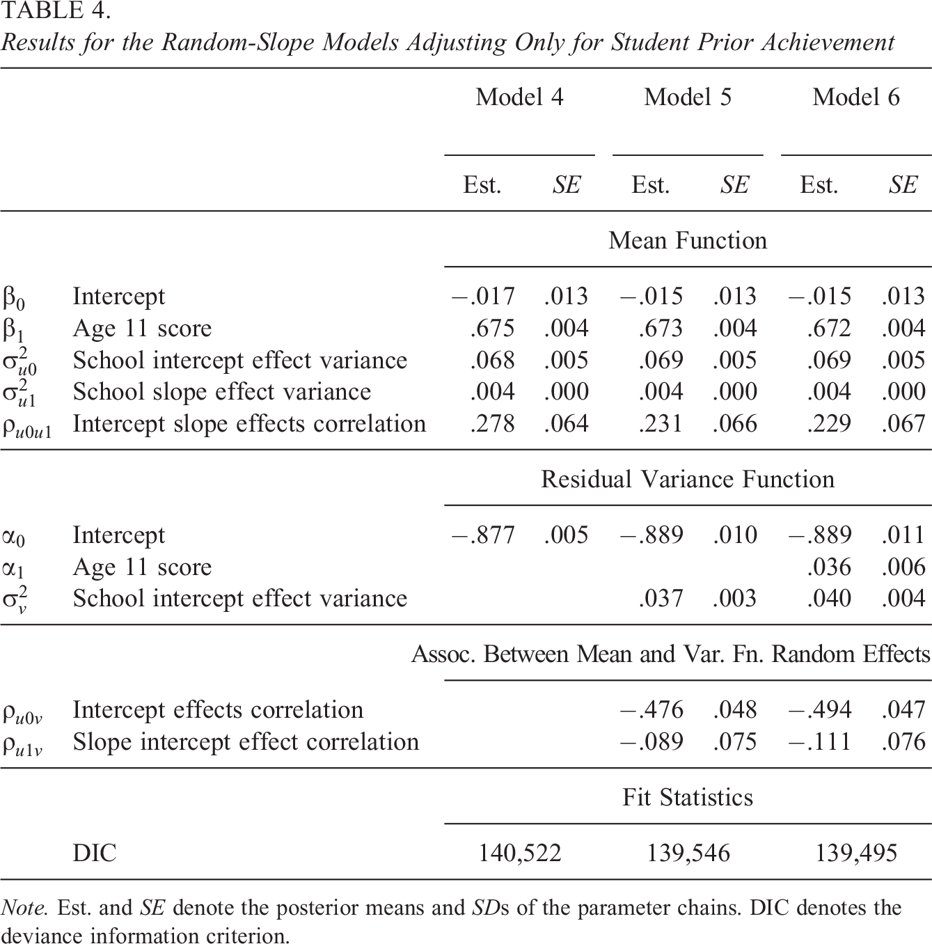
Note. Est. and SE denote the posterior means and SDs of the parameter chains. DIC denotes the deviance information criterion.
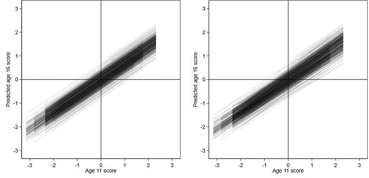
Model 1 and Model 4 school regression lines of predicted age 16 scores against age 11 scores for random-intercept model (left) and random-slope model (right).
Model 5: Random-Slope Model With Random Residual Variance
Model 5 (Equation 5) extends the random-slope model (Model 4, Equation 4) to allow the residual variance to vary across schools. Thus, the move from Model 4 to 5 for the current random-slope model mirrors the move we explored from Model 1 to 2 for the earlier random-intercept versions of these models.
Model 5 allows us to quantify the relative importance of the differential school effects with respect to prior achievement as a component of the overall variance in student adjusted achievement in each school. We calculate the estimated variance for each school in our sample for a common reference distribution of students with student age 11 score variance
Model 6: Random-Slope Model With Random Residual Variance Function
Model 6 (Equation 6) further extends the random-slope model to allow the residual variance to vary not just across schools (Model 5, Equation 5), but additionally as a function of student prior achievement. Thus, the move from Model 5 to 6 for the current random-slope model mirrors the move we explored from Model 2 to 3 for the earlier random-intercept versions of these models. As with the sequence of random intercept models, Model 6 shows the residual variance in the random-slope model significantly increases with student age 11 scores
Model 7: Random-Intercept Model With Random Variance Function and Student Characteristics
Model 7 extends Model 3 by adding student age, gender, first language, special educational need (SEN) status, and FSM status into the mean and residual variance functions (Table 1). Adding these characteristics to the mean function implies students are now compared to other students across London who not only share the same age 11 score, but who also share the same sociodemographic characteristics. The aim is to ensure that schools do not appear more or less effective simply as a result of recruiting more or less educationally advantaged students (Leckie & Goldstein, 2019). The resulting improved accuracy of the predicted age 16 scores will lead the student adjusted achievement scores to in general reduce in absolute magnitude (and reorder) leading the overall variance in student adjusted achievement to decrease. In turn, the school means and variances of student adjusted achievement scores will also change, again in general reducing in magnitude and reordering. We then further adjust the school variances of student adjusted achievement by including the student characteristics in the student residual variance function. This ensures that if there are any London-wide relationships between the variance in student adjusted achievement and particular student characteristics, this again will not benefit or count against schools with disproportionate numbers of these students.
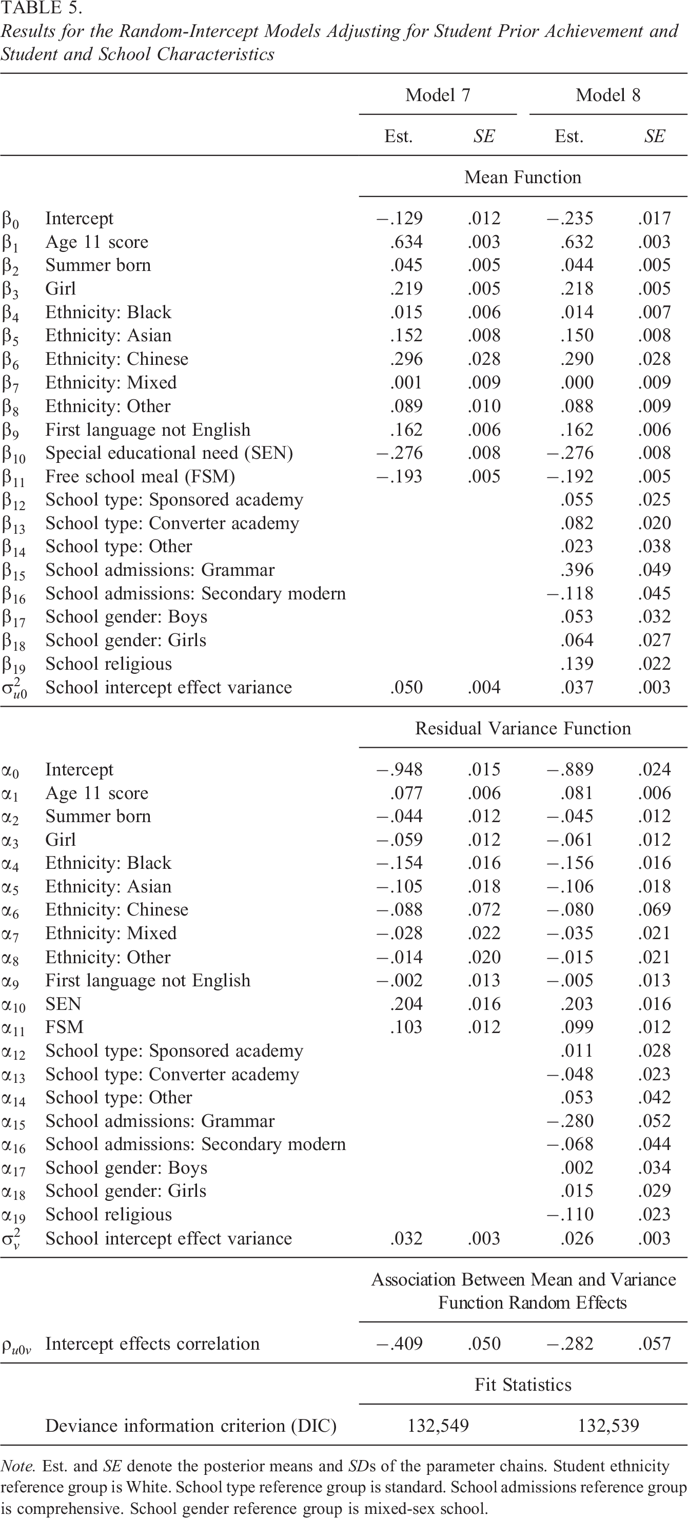
Table 5 presents the results. Model 7 is preferred to Model 3 (
Results for the Random-Intercept Models Adjusting for Student Prior Achievement and Student and School Characteristics
Note. Est. and SE denote the posterior means and SDs of the parameter chains. Student ethnicity reference group is White. School type reference group is standard. School admissions reference group is comprehensive. School gender reference group is mixed-sex school.
Figure 6 presents the scatterplots of the school means and variances of student adjusted achievement based on the current model, which adjusts for student background against those based on Model 3 which ignores student background. The purpose of this figure is to explore the sensitivity of the school means and variances to the additional adjustments for student background and to therefore assess the importance of making such adjustments or not (Leckie & Prior, 2022; Levy et al., 2023). We calculate the estimated school variances in each model by plugging in the sample mean values for the covariates (Table 1) in the residual variance function, and so,
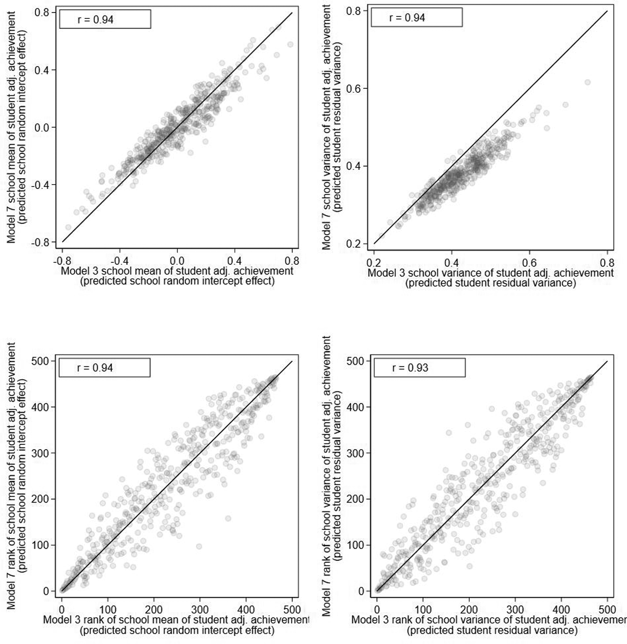
Model 7 against Model 3 scatterplots of school means of student adjusted achievement (top left), school variances of student adjusted achievement (top right), ranks of school means of student adjusted achievement (bottom left), and ranks of school variances of student adjusted achievement (bottom right).
Model 8: Random-Intercept Model With Random Variance Function and School Characteristics
We now shift from attempting to best define and measure student adjusted achievement, and therefore the school means and variances of student adjusted achievement, to attempting to explain why some schools show higher mean student adjusted achievement and lower variance in student adjusted achievement than others. Unfortunately, we do not observe school policies and practices in our data. However, we do observe some school characteristics (Table 2). Model 8 extends Model 7 by adding school type, school admissions, school gender (mixed, boys, and girls), and school religion to the mean and residual variance functions.
The results (Table 5) for the existing mean and residual variance function regression coefficients are very similar to before and so we restrict our interpretation here to the new results. First, consider the mean function. Relative to standard school types, school mean adjusted achievement is somewhat higher in sponsored and converter academies having adjusted for the other covariates. Similarly, school mean adjusted achievement is higher in girls’ schools and religious schools, all else equal. However, the most sizable differential is related to school admissions: School mean adjusted achievement is considerably higher in grammar schools and lower in secondary modern schools relative to comprehensive schools. These results agree with the literature (Leckie & Goldstein, 2019). With respect to the residual variance function, we see new findings. School variances in student adjusted achievement tend to be lower in converter academies compared to standard school types, lower in grammar schools versus comprehensive school types, and lower in religious schools versus nonreligious schools, and this is after adjusting for London-wide relationships between the variance in student adjusted achievement and student characteristics. Thus, students in converter academies, grammar, and religious schools not only tend to show higher student adjusted achievement on average but also tend to show more consistent student adjusted achievement.
5. Discussion
In this article, we have argued that the focus of school value-added models should broaden to measure not just school mean differences in student adjusted achievement (student achievement beyond that predicted by student prior achievement and other student background characteristics), but school variance differences in student adjusted achievement. To study school variance differences, we have proposed extending the traditional school value-added model, a random-intercept mixed-effects linear regression of student current achievement on prior achievement and other student background characteristics, by modeling the residual variance as a log-linear function of the student covariates and a new random school effect. The school random intercept effect and random residual variance in this model measure the school mean and variance in student adjusted achievement. This model can be viewed as an application of the MELS model popular in biostatistics (Hedeker et al., 2008). It is, however, important to reiterate that the school value-added models and their respective predicted school effects should be viewed as descriptive rather than causal since these models do not address the complex selection into schools processes that will be in play in many school systems.
We have illustrated this extended school value-added model with an application to schools in London. In response to our research question: Our results suggest meaningful differences in the variance in student adjusted achievement across schools. We also find a moderate to large negative association between the school mean and variance in student adjusted achievement. Thus, schools that show the highest mean student adjusted achievement also tend to be the schools that show the lowest variance in student adjusted achievement. One process by which school variance differences may arise is if there is a London-wide negative relationship between the variance in student adjusted achievement and student prior achievement. We adjusted for this by entering student prior achievement into the residual variance function. A second process by which school variance differences may arise is via interaction effects between the different school policies and practices envisaged to be represented by the school random intercept effect and observed and unobserved student characteristics. Previous research has studied this via entering a school random slope on student prior achievement and this showed schools to be differentially effective for students with low, middle, and high prior achievement. In our application, however, these school-by-student prior achievement interactions are small and explain little of the variation in school variances between schools. We then turned our attention to entering student characteristics into the model, both in the mean and residual variance functions, to better measure student adjusted achievement. In terms of new results, we find that FSM and SEN students show greater variance in student adjusted achievement and therefore less predictable age 16 scores than otherwise equal students. The resulting predicted school means and variances of student adjusted achievement, however, are similar to those based on the model, which only adjusts for student prior achievement. Nevertheless, schools whose sociodemographic student mix differ most from the average school still move up and down the London-wide rankings considerably, demonstrating the importance of adjusting for student background at least for some schools (Leckie & Goldstein, 2019; Leckie & Prior, 2022; Levy et al., 2023). Finally, we shifted our emphasis from measuring school means and variances of student adjusted achievement to seeking to explain them. We find converter academies and grammar schools tend to show lower variances in student adjusted achievement than other school types. Importantly, here too we adjusted for any overall relationship between the variance in student adjusted achievement and student prior achievement and background characteristics, and so, these differences in school variances lie beyond this simple explanation.
Future studies might seek to identify whether school variance differences can be predicted by specific school policies and practices. It will also be interesting and important to explore the role of school composition covariates, such as the school mean and school SD of the student prior achievement (Raudenbush & Bryk, 2002). One issue that such studies should bear in mind is that some student current achievement measures may exhibit floor or ceiling effects. Where these are pronounced, they may bias the model parameters relative to fitting models to measures without such effects. Tobit versions of the models might be considered to address this issue (Lu, 2018). Another issue is sample-size requirements. In general, we found that the residual variance function regression coefficients and predicted school effects were less precisely estimated than their analogous quantities in the mean function. This suggests that larger sample sizes are needed for these models than traditionally used for school value-added studies. Future studies might therefore use power calculations to guide such decisions (Walters et al., 2018).
More generally, however, expanding the focus of school value-added models to consider schools effects on the variance in student achievement raises value judgements and interpretational challenges that future work will need to engage with. Fundamentally, it is not clear how positively or negatively higher or lower variances should be viewed in general. Similarly, where a given school policy or practice is identified as driving school differences in variance via differential effects on students as a function of their observed and unobserved characteristics, it will not typically be clear what the optimal degree of differential impact might be. Even if it is decided that higher variance should be interpreted in a particular way, faced now with two summaries of school effects on student learning (mean and variance effects), researchers and school accountability systems must make further value judgments as to how to best combine them into any overall summary of school effectiveness for the purpose of making overall inferences, judgements and decisions about schools (Prior, Goldstein, et al., 2021). Crucially, it is only by extending the school value-added model to allow for school effects on the variance in student adjusted achievement that such debates are made possible. The extension we have presented paves the way for new substantive research into the reasons behind differences in variability and therefore how best such differences should be interpreted and addressed.
The school value-added model presented here can be further extended in various ways beyond simply adding further covariates and random slopes suggesting avenues for new methodological research. First, in the school effectiveness literature, there is interest in studying the consistency of school effects across academic subjects (Goldstein, 1997; Reynolds et al., 2014; Teddlie & Reynolds, 2000). We can further develop the school value-added model to study this phenomenon with respect to the school variance in student adjusted achievement. Essentially, we would fit a multivariate response version of this model for multiple student achievement scores (Kapur et al., 2015; Leckie, 2018; Pugach et al., 2014). The model would have multiple residual variance functions, one for each academic subject. We can then study the correlations of the school means and variances of student adjusted achievement across subjects. Second, the same multivariate response version of the model can be used to study the stability of school effects over time. Here, we would fit a multivariate response model to a single achievement score, but for multiple student cohorts (Leckie & Goldstein, 2009). Third, we could include a random slope in the residual variance function (Goldstein et al., 2018; McNeish, 2021) to study whether schools exacerbate or mitigate any overall relationship between the variance in student adjusted achievement and student prior achievement. Fourth, while we have flexibly modeled the residual variance, we have not modeled the random intercept variance (the random slope model relaxed this, but in a rather specific way). It is also possible to model the random intercept variance as a log-linear function of school covariates (Hedeker et al, 2008). For example, the variability of school mean adjusted achievement scores across schools may appear greater for some school groups than others, and this could then be tested by introducing the school group variable as a covariate in this second variance function. Fifth, we can expand the model to three levels to incorporate an additional random effect into the mean and residual variance functions relating to, for example, school district and thereby study school district differences in the mean and variance in student adjusted achievement. This then raises the possibility of entering school district random effects into the school random intercept variance function since school mean adjusted achievement might vary more in some school districts than in others, and so with this extension, we can potentially study differential school-level inequalities in the education system by school district (Leckie et al., 2012; Leckie and Goldstein, 2015). Alternatively, teacher random effects could be introduced as a new level between the student and school level. Finally, our focus has been on shifting attention from studying school mean of student adjusted achievement to additionally focusing on the variance in student adjusted achievement. In future work, it would be interesting to explore further ways the distribution of student adjusted achievement might vary across schools, for example, with respect to skewness.
Supplemental Material
Supplemental Material, sj-do-1-jeb-10.3102_10769986231210808 - Mixed-Effects Location Scale Models for Joint Modeling School Value-Added Effects on the Mean and Variance of Student Achievement
Supplemental Material, sj-do-1-jeb-10.3102_10769986231210808 for Mixed-Effects Location Scale Models for Joint Modeling School Value-Added Effects on the Mean and Variance of Student Achievement by George Leckie, Richard Parker, Harvey Goldstein and Kate Tilling in Journal of Educational and Behavioral Statistics
Supplemental Material
Supplemental Material, sj-docx-1-jeb-10.3102_10769986231210808 - Mixed-Effects Location Scale Models for Joint Modeling School Value-Added Effects on the Mean and Variance of Student Achievement
Supplemental Material, sj-docx-1-jeb-10.3102_10769986231210808 for Mixed-Effects Location Scale Models for Joint Modeling School Value-Added Effects on the Mean and Variance of Student Achievement by George Leckie, Richard Parker, Harvey Goldstein and Kate Tilling in Journal of Educational and Behavioral Statistics
Supplemental Material
Supplemental Material, sj-dta-1-jeb-10.3102_10769986231210808 - Mixed-Effects Location Scale Models for Joint Modeling School Value-Added Effects on the Mean and Variance of Student Achievement
Supplemental Material, sj-dta-1-jeb-10.3102_10769986231210808 for Mixed-Effects Location Scale Models for Joint Modeling School Value-Added Effects on the Mean and Variance of Student Achievement by George Leckie, Richard Parker, Harvey Goldstein and Kate Tilling in Journal of Educational and Behavioral Statistics
Supplemental Material
Supplemental Material, sj-r-1-jeb-10.3102_10769986231210808 - Mixed-Effects Location Scale Models for Joint Modeling School Value-Added Effects on the Mean and Variance of Student Achievement
Supplemental Material, sj-r-1-jeb-10.3102_10769986231210808 for Mixed-Effects Location Scale Models for Joint Modeling School Value-Added Effects on the Mean and Variance of Student Achievement by George Leckie, Richard Parker, Harvey Goldstein and Kate Tilling in Journal of Educational and Behavioral Statistics
Footnotes
Authors' Note
This work contains statistical data from Office for National Statistics (ONS), UK, which is Crown Copyright. The use of the ONS statistical data in this work does not imply the endorsement of the ONS in relation to the interpretation or analysis of the statistical data. These data are not publicly accessible, but researchers can apply to analyze them ![]() .
.
Declaration of Conflicting Interests
The author(s) declared no potential conflicts of interest with respect to the research, authorship, and/or publication of this article.
Funding
The author(s) disclosed receipt of the following financial support for the research and/or authorship of this article: This research was funded by UK Economic and Social Research Council (ESRC) grants ES/R010285/1 and ES/W000555/1 and UK Medical Research Council (MRC) grants MR/N027485/1 and MC_UU_00032/02.
References
Supplementary Material
Please find the following supplemental material available below.
For Open Access articles published under a Creative Commons License, all supplemental material carries the same license as the article it is associated with.
For non-Open Access articles published, all supplemental material carries a non-exclusive license, and permission requests for re-use of supplemental material or any part of supplemental material shall be sent directly to the copyright owner as specified in the copyright notice associated with the article.