
Abstract
Research on academic performance typically revolves around average achievement scores of students or schools. Focusing solely on averages can miss important aspects of the learning experience. The recent development of mixed-effects location scale models (MELSM) has provided a modeling technique that incorporates a scale model that captures and explains the consistency of academic achievement within the cluster of interest. Here, we formally introduce an extension to the MELSM, a Spike-and-Slab Mixed-Effects Location Scale Model (SS-MELSM), for simultaneously modeling location and scale parameters while incorporating a spike-and-slab prior to select or shrink random effects. Our approach identifies clusters with unusually large or small within-cluster variance in academic achievement, which can indicate overly inconsistent or consistent outcomes. To assess the performance of the proposed method, we conducted a simulation study, followed by an application to a dataset of 160 schools from the Brazilian Evaluation System of Elementary Education (Saeb) to illustrate its use in educational data analysis. Moreover, we show how to compare models with varying parameters regarding expected predictive accuracy. The results demonstrate that the SS-MELSM successfully identifies schools with unusually high and low consistency in mathematics achievement and that school- and student-level SES were relevant covariates when modeling the location and scale components. The methods presented in this paper are implemented in the R package ivd.
Keywords
Research on academic performance typically focuses on the average academic achievement of a student or a school (or other clustering units such as classrooms, districts, counties, etc.). While average performance is indubitably an important metric for academic achievement, it provides an incomplete picture. Specifically, it does not provide information on the variability or the consistency of academic achievement over time or within a cluster. To illustrate the distinction between average academic achievement and consistency, we can concoct a very simple example consisting of two hypothetical schools in which students take a standardized exam: Both schools achieve the same average score of 75% among their students, suggesting a similar academic performance. However, the consistency of student performance within each school could vary greatly. In one school, individual student scores may range widely from 50% to 100%, while the other school’s student scores cluster around 75%. Although the two schools have the same average score, their students’ experiences and levels of mastery of different topics are almost certainly different.
Capturing cluster-level variability alongside the average score offers a more comprehensive view of academic achievement, with both metrics providing unique insights that can guide more targeted student or school-specific evaluations and support. The idea that average performance and variability convey distinct information is by no means a novel one, and it has been discussed at the levels of students and at the level of school classes and schools.
At the school level, Raudenbush and Bryk (1987) developed a statistical framework to study how organizational characteristics predict variability in academic achievement. Their work showed that dispersion in outcomes is not just statistical noise. Instead, these differences can reveal whether schools help reduce or increase inequality. Socioeconomic status (SES) is a key factor that affects differences both within and between schools. A student’s family SES influences their access to resources and learning opportunities, which affects their achievement and persistence (Lurie et al., 2021; Tompsett & Knoester, 2023; von Stumm et al., 2022). At the same time, the school-level SES, which often reflects patterns of residential and financial segregation, shapes the availability of resources, teacher quality, and curriculum offerings (Perry et al., 2022; Sirin, 2005). These factors lead to large differences between schools in both average achievement and the extent of achievement variation, with lower-quality schools often worsening socioeconomic inequality, while higher-quality schools can sometimes help reduce it (Borgen et al., 2025). Teacher biases against students from lower-SES backgrounds and differences in how schools are organized, such as school size or the range of math courses offered, can also affect how much achievement varies within schools (Doyle et al., 2023).
The idea of using dispersion as a meaningful metric appears in other achievement research as well. For instance, research by Brunner et al. (2013) shows that gender differences in academic achievement are complex. While boys and girls often have similar average achievement, boys tend to show greater variability. As a result, boys are more likely to be overrepresented at both the highest and lowest achievement levels. These results highlight why it is important to look at both average performance and consistency to better understand achievement and guide interventions.
A related, though conceptually distinct, line of research has examined variability at the individual level. For example, Connell and Wellborn (1991) found that consistency in academic performance is associated with better psychological engagement and motivation in students. Similarly, Gottfried et al. (2008) showed that students with more consistent academic performance achieve higher test scores and are more likely to enroll in college. By contrast, other work, such as Wright and von Stumm (2022), questioned the predictive utility of within-person grade variability, showing in a twin study that it did not forecast later educational outcomes.
While these studies of within-person variability are informative, the focus of the present work returns to the within-cluster level. Overall, inconsistent performance may reflect unaccounted factors influencing learning. Detecting such variability can uncover potential learning barriers, optimize individualized teaching strategies, and possibly improve educational outcomes. Moreover, understanding the nature of inconsistency may shed light on systemic issues within the school environment that not only affect academic outcomes but also contribute to students’ social and emotional development (Spörlein & Schlueter, 2018).
In this work, we present an approach that identifies clustering units (students, classrooms, etc.) that exhibit either unusually large or unusually small within-cluster variance – indicating either consistent or inconsistent academic achievement. As such, the goal of this current paper is not to settle the discussion on whether within-cluster variance is predictive of future educational outcomes, but to present a tool that allows researchers to identify and isolate clusters (such as students, classrooms, schools, etc.) that display unusual amounts of residual variability. A similar idea has been put forth by Leckie et al. (2023), who used school-specific expected residual variance from a mixed-effects location scale model (MELSM) to identify variables that contribute to inconsistency in academic achievement and to refine school value-added models. The MELSM approach allowed them to rank order schools in terms of within-school variance (see also Brunton-Smith et al., 2017). The work presented here shares the same general approach of modeling residual variances in a MELSM. Our focus, however, is on the identification of clustering units that show unusually high or low consistency in academic achievement, rather than systematically studying predictors of variability.
In order to identify clusters (students, classes, schools, etc.) with unusual consistency in academic achievement, we present an adaptation of the MELSM by means of shrinking random effects to their fixed effect using the spike-and-slab regularization technique (George & McCulloch, 1993, 1997; Kuo & Mallick, 1998) that has been fruitfully applied in the context of the selection of random effects in classic multilevel models (Frühwirth-Schnatter & Wagner, 2011; Rodriguez et al., 2022; Williams et al., 2021). The spike-and-slab prior serves as the Bayesian analog to lasso regularization, but it allows one to combine it with Bayes factors that provide a decision boundary for the identification of clusters with unusually large or small residual variability.
The remainder of the manuscript is organized as follows. First, we review and formally describe the MELSM for multilevel-type data. Second, we introduce the novel Spike-and-Slab MELSM (SS-MELSM), which identifies clusters that are unusually consistent or inconsistent in their academic achievement, which will also be referred to as atypical schools for ease of exposition throughout this manuscript. Next, we conduct a simulation study to evaluate the SS-MELSM accuracy in finding clusters with unusual residual variability, and compare it to a two-stage hierarchical linear model (HLM). Finally, we provide an example involving empirical data from Brazil’s Elementary Education Evaluation System (Instituto Nacional de Estudos e Pesquisas Educacionais Anísio Teixeira, 2021). We conclude by discussing the findings in the context of educational research and pointing out possible limitations and extensions of the SS-MELSM.
MELSM for Educational Data
Educational data are typically analyzed using multilevel or mixed-effects models (MLM) that partition between- and within-cluster variance. In the examples presented throughout this paper, the clustering level 2 refers to schools, while the level-1 units are students within schools.
MLMs capture the expected mean response conditioned on clustering levels and predictors situated at different levels of analysis. The standard assumption in the MLM is one of constant error variance, and consequently, the residual variance, or scale part of the MLM, is left unmodeled (Raudenbush & Bryk, 2002). This assumption can be relaxed using so-called MELSM that include a submodel to address potential differences in the residual variance that lead to cluster-specific heteroskedasticity (Hedeker et al., 2008; Leckie et al., 2014; Rast et al., 2012). The idea behind these models is that the unexplained residual variance is not merely Gaussian white noise but that it still contains some degree of information about the student or, more generally, the clustering unit that can be modeled and explained. Specifically, the nature of the variability itself might provide insights over and above the expected academic achievement captured in the conditional means or location. MELSMs are relatively new in the context of educational research (Goldstein et al., 2018; Leckie et al., 2014, 2023), but the idea that the nature of the residual variance structure itself contains behavioral information has been entertained for a long time (see Rausch, 1948; Woodrow, 1932).
The MELSM allows the simultaneous estimation of a model for the means (location) and a model for the residual variance (scale). Both these submodels allow the inclusion of specific predictors and are conceptualized as mixed-effect models. As with any multilevel model, the MELSM addresses the nested structure of typical educational data by estimating fixed and random effects for the location and the scale while including predictors at the respective levels. A distinguishing feature of the MELSM is the simultaneous estimation of the means and the residual variance part of the model, allowing random effects of both location and scale to correlate. In other words, the model specifies a classic multilevel model for the observed values, y
ij
for school j and student i, and a multilevel model for the within-cluster residual variances
To keep the model description in line with our examples, we show the models with the clustering unit School at Level 2 and the achievement score for Students at Level 1. The starting point is the standard linear MLM for
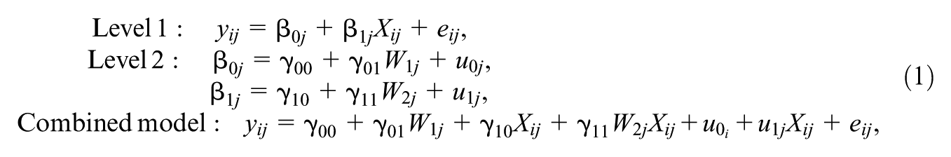

The combined model is given in Equation (1), where y
ij
captures the achievement score for student i within school j, and X
ij
is a predictor that can contain school or student-level information. The fixed effects coefficients are captured by the
It’s important to note that in this standard model, the within-school or residual variance
This relation is shown in the scale model
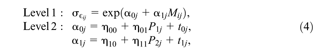
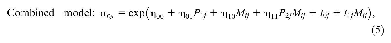
where
Comparable to the regression weights in Equation (1),
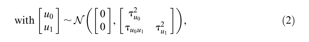
We now have random effects u0j and u1j from the location of the model (the means structure) and random effects t0j and t1j from the scale of the model (the within-cluster standard deviation structure). All these random effects are assumed to come from the same multivariate Gaussian Normal distribution with zero means and covariance matrix
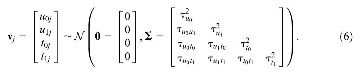
Here,
Alternatively, we can express the relation among the random effects on the location and scale models via the Cholesky parameterization (Hedeker et al., 2008). This parameterization facilitates the inclusion of a variable selection mechanism presented later in the Spike and Slab MELSM section, ensures positive-definiteness, and improves the efficiency of Hamiltonian Monte Carlo (HMC) estimation. That is,
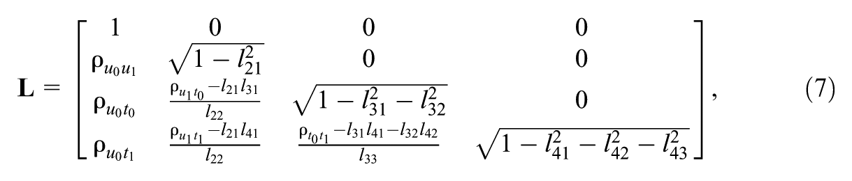
where ρ is the correlation between the subscripted random effects and l
nm
are the elements in

The individual elements of
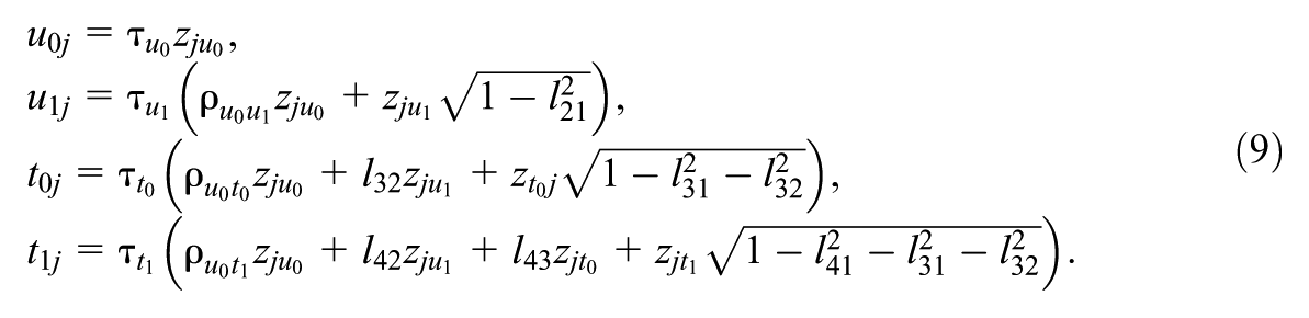
Equation (9) demonstrates how the Cholesky decomposition allows us to express the four random effects in our example model in terms of the standard deviations and correlations. This approach is particularly useful in complex models like MELSM, where both the mean and variance structures are modeled jointly.
From a Bayesian modeling perspective, so far, we have defined the likelihood part of the MELSM in Equations (1) and (5), which can be written concisely in matrix notation

Here,
When specifying a Bayesian model, we assign prior probability distributions to the parameters of interest. The priors for the fixed effects parameters are given as


The priors for the random effect parameters in


where
To summarize, by estimating a joint model for both the location and the scale components simultaneously, we are able to account for possible correlations that arise among location and scale effects, ensuring that we can make valid inferences about parameter estimates (Leckie, 2014; Verbeke & Davidian, 2009). Hence, in the MELSM, we do not need to assume that the residual standard deviation is homogeneous across all Level-1 units. Rather, the variability can be conditional on predictor variables, such as school-level or student-level variables, and it effectively models heteroskedastic processes. For example, the variability of student performance within a school can be modeled as a function of parental SES, with the assumption that low SES leads to more variability in student achievement. In other words, a student from a lower socioeconomic background might be associated with larger residual standard deviations and less consistent achievement. Consequently, its performance will be more difficult to estimate reliably while controlling for school-level effects (for different MELSM examples, see Brunton-Smith et al., 2017; Martin & Rast, 2022; Williams et al., 2021).
The MELSM allows one to estimate residual standard deviations that vary both at the school- and the student level. This distinction forms the foundation for the next steps, where we introduce a Bayesian variable selection method capable of identifying schools (clusters) whose student-level residual standard deviations are not captured well by scale fixed effects. This approach helps pinpoint schools that produce students with inconsistent academic achievement. It aligns with the idea presented by Leckie et al. (2023) that focuses on estimating different school-level standard deviations. However, our method differs by employing a Bayesian model selection approach to identify key schools (clusters). Specifically, we use the spike-and-slab approach, allowing the model to switch between two assumptions for each school: one that assigns a high probability to a common error standard deviation (
Spike and Slab MELSM
With the Cholesky parameterization of the covariance matrix in Equation (7) at hand, we can now introduce a selection mechanism to the MELSM based on the Bayesian spike-and-slab regularization technique (Frühwirth-Schnatter & Wagner, 2011; Kuo & Mallick, 1998; Mitchell & Beauchamp, 1988). This addition gives rise to the SS-MELSM. That is, Equation (8) can be expanded to include an indicator vector

Accordingly, we can include the individual elements
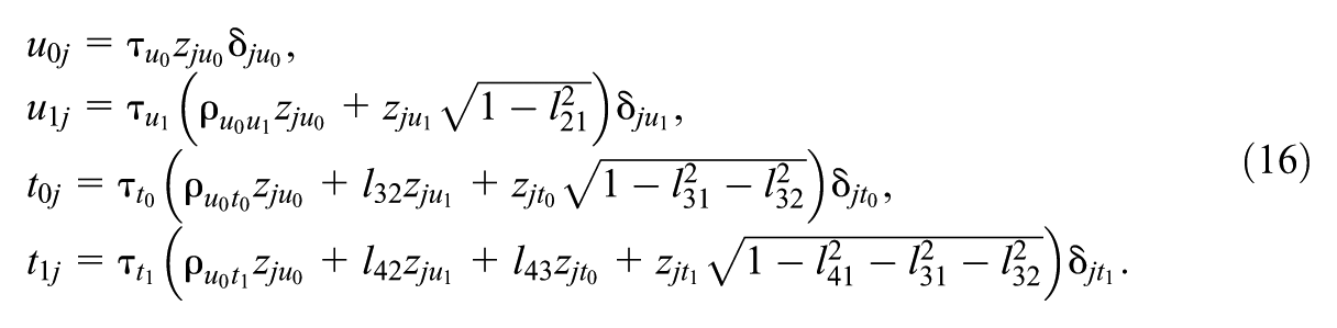
Each element in
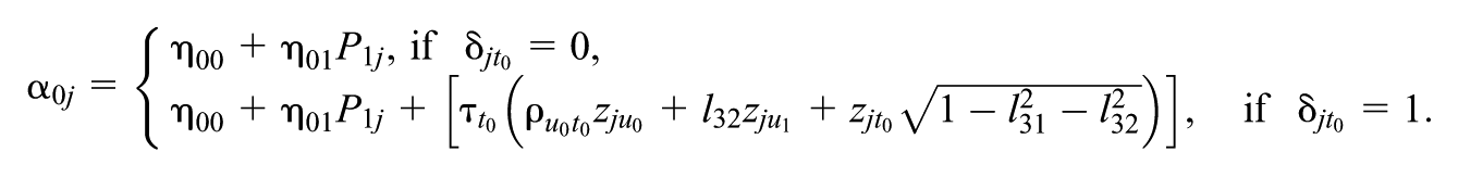
In this context, the indicator vector
The prior probability of retaining the k’th random effect is given by the parameter
Combining the prior Bernoulli distribution with the standard normal prior defined for
Note that Equation (15) and example (16) introduce the spike-and-slab as j vectors, each of length k that potentially shrink all random effect deviations from the fixed effects in both the location and the scale part of the model. Given that the focus of this paper is on identifying clusters with large departures from the average residual standard deviation, we limit ourselves in the remainder of this work to including the spike-and-slab on the scale model only. This is easily achieved by constraining the
Posterior Inclusion Probability
In the context of spike-and-slab models, the posterior inclusion probability (PIP) quantifies the probability that a given random effect is included in the model, conditional on the observed data,
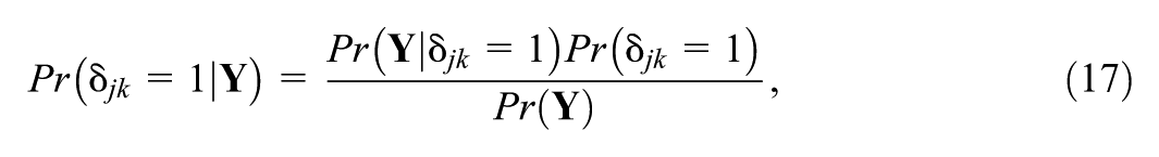
where
In practice, the PIP can be directly estimated from the Markov Chain Monte Carlo (MCMC) sampling approach. For each iteration (s) of the MCMC chain, the indicator variable
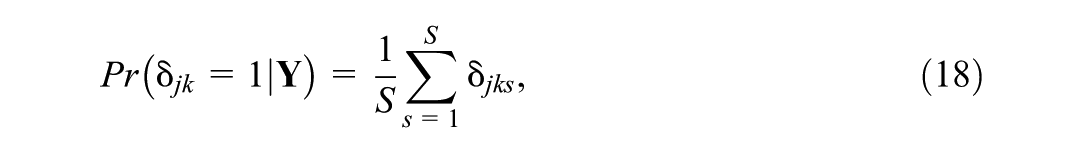
where S is the total number of posterior samples. The subscript j on the indicator variable (
While the PIP gives us a probabilistic measure of whether a random effect should be included or not, it does not perform automatic variable selection. To determine whether a given random effect is warranted, we follow Williams et al. (2021) and Rodriguez et al. (2022) by estimating the strength of evidence through Bayes factors (Rouder et al., 2018)
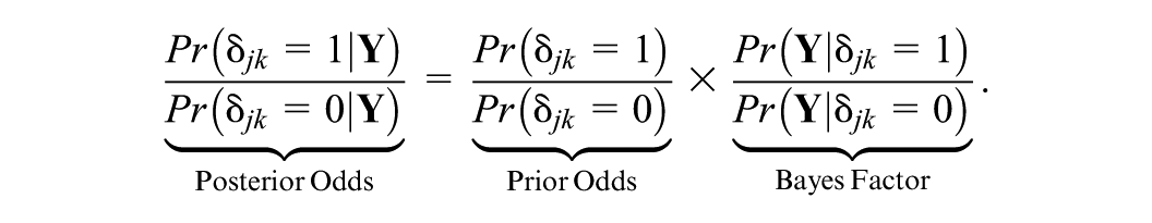
Setting the prior probability of
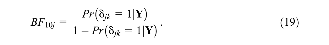
By calculating PIPs and Bayes factors, we can quantify the evidence supporting whether a school’s standard deviation differs from the average within-school standard deviation. It is common practice to interpret a Bayes factor greater than three as substantial evidence in favor of the target hypothesis (Kass & Raftery, 1995).
Simulation Study
In this section, we present a simulation study to evaluate the SS-MELSM’s performance in correctly identifying clusters (schools) with unusual within-cluster variability. We aim to evaluate the method’s classification accuracy as well as its ability to recover the data-generating parameters under various conditions. In addition, we compare SS-MELSM to a two-stage V-known HLM, as proposed by Raudenbush and Bryk (1987). This is a framework where the sampling variance for each school’s dispersion estimate is treated as a known quantity in the second stage of the analysis. This method first calculates a transformed measure of dispersion for each school and then, in a second stage, models these measures to produce shrunken estimates. A school is identified as atypical if its standardized residual falls outside the 95% confidence intervals of the expected normal distribution.
Data for this study were generated from the following model:
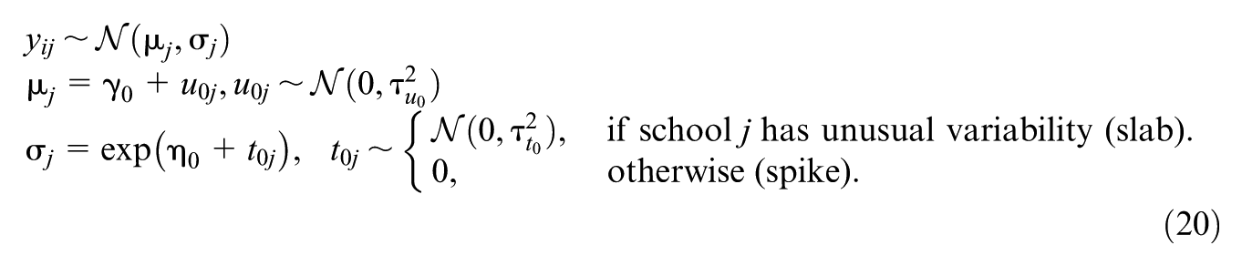
This model defines the outcome, y
ij
, for student i in school j via the fixed intercept parameter
We fixed
We defined the effect size for the slab standard deviations (
To assess performance in more challenging small-sample scenarios where the benefits of shrinkage in the HLM are particularly relevant, we conducted a targeted secondary simulation. In this study, we varied the average number of students per school to
In each simulated dataset, atypical schools were randomly selected with probability
Software and Estimation
The SS-MELSM relies on Bayesian estimation approaches, as computing PIPs through the spike and slab method is inherently Bayesian. In order to obtain the elements in
Spike-and-Slab MELSM
The fitted MESLM follows the data-generating model shown in Equation (20). This model’s formulation contains only two random effects: one for the location and another for the scale part. In this case, the spike and slab indicator
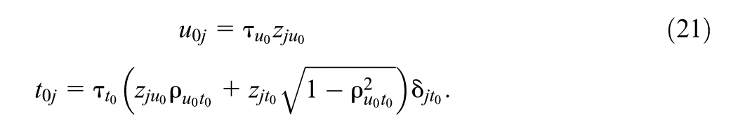
We define the priors for the parameters in Equation (21) as


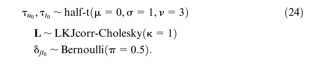
We assign uninformative normal priors to the fixed effects, as indicated by the large prior variances in Equation (23), and by the degrees of freedom of the random effects standard deviation (ν= 3) in Equation (24). For the Cholesky factor

As shown in Equation (18), this setup allows us to compute the PIP of the random effects and assess the relative evidence for its inclusion using the Bayes factor (Equation 19), assuming equal prior odds for the spike and slab components. We consider
All models were fitted with three chains of 2,000 iterations and 1,000 warm-up samples. The number of iterations was chosen to ensure good quality of the parameter estimates, with the models converging as indicated by potential scale reduction factors
Two-Stage HLM
As a baseline for comparison, we also fitted a two-stage HLM, following the large-sample approach detailed by Raudenbush and Bryk (1987). Similar to the MELSM, this framework also defines a model for the residual variance as an outcome, but the location and scale models are estimated separately in two stages.
First, a standard random-intercept MLM is fitted to the student-level data. From this model, we calculate a bias-corrected, log-transformed measure of dispersion for each school j:

where
In the second stage, these d
j
values are treated as the outcome in a hierarchical model with known variance. This model yields empirical Bayes estimates (
To identify schools with unusual variability, we standardized these empirical Bayes residuals to obtain Z j and constructed a normal Q-Q plot of the resulting values. A school was flagged as having an extreme level of dispersion if its Z j value fell outside the 95% confidence bands of the Q-Q plot. This approach identifies only those schools whose variability is statistically inconsistent with the overall distribution.
Performance Metrics
For each simulated dataset, we computed the set of schools truly belonging to the slab group, as determined by the data-generating mechanism. We then compared this to the set of schools flagged by each method as having unusual within-cluster variance.
Using the flagged and true slab schools, we computed the sensitivity, specificity, and precision for each method:
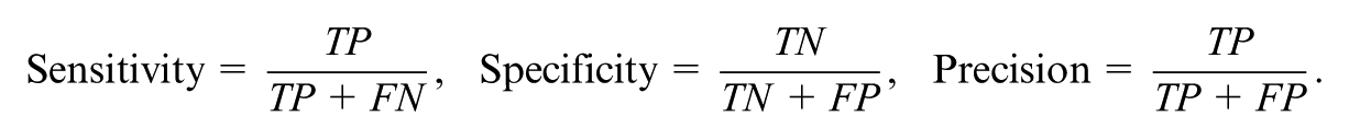
TP and FP are the number of true and false positives, respectively, whereas TN and FN are the number of true and false negatives, respectively. We used these rates to compute the F1 score (Powers, 2020), which is the harmonic mean of precision and sensitivity. It is defined as

We focus on the F1 score because, while we hope to maximize the identification of true positives, a false positive in an educational context can have relevant consequences. For example, it can initiate unnecessary and expensive investigations, diverting finite administrative time, funding, and support personnel away from schools that genuinely require intervention.
We also evaluated the quality of parameter recovery for the standard deviation of the scale random effect,
Results
Primary Simulation Study
Parameter Recovery
Our primary simulation evaluated the SS-MELSM’s ability to recover the standard deviation of the scale random effect,
Interestingly, increasing the number of students per school did not uniformly reduce bias but rather amplified some existing patterns. In a condition prone to overestimation (
Classification Performance
To evaluate the ability of each method to correctly classify schools as belonging to the “spike” or “slab” group, we assessed sensitivity, specificity, and the F1 score. Visual inspection of these metrics revealed that their distribution was primarily driven by the number of students and the effect size, while being roughly invariant to the number of schools. Therefore, we focus our illustrative results on the conditions with 150 schools.
Both methods demonstrated reasonably good sensitivity, which improved with larger effect sizes. However, as shown in Table 1, the two-stage HLM was often slightly more sensitive, particularly in conditions with more students and a higher proportion of atypical clusters. For example, with 150 schools,
Average Values of Sensitivity and Specificity for SS-MELSM and Two-Stage HLM, Including only Conditions of 150 Schools
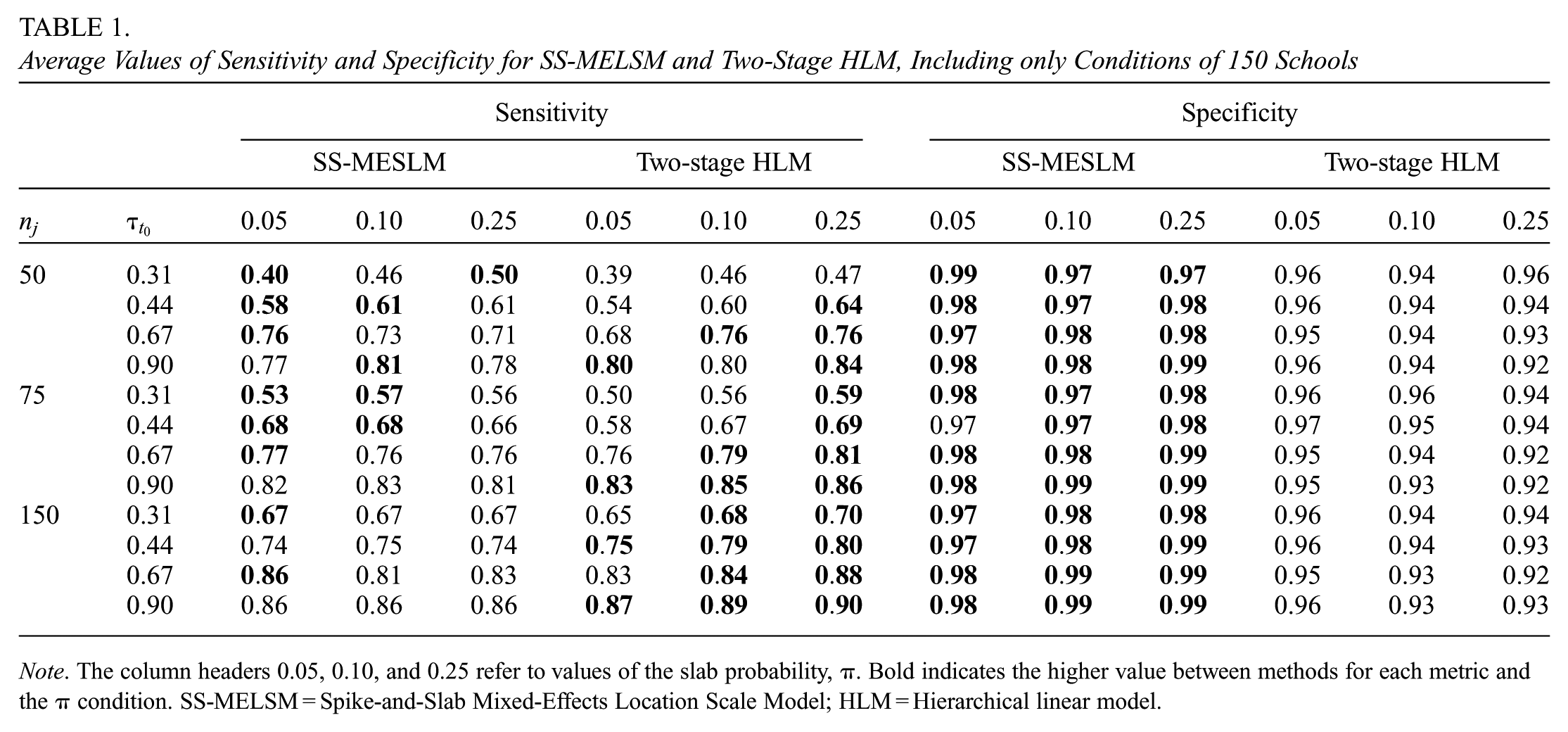
Note. The column headers 0.05, 0.10, and 0.25 refer to values of the slab probability,
On the other hand, the SS-MELSM was consistently better at avoiding false positives, maintaining a high and stable specificity across all conditions. For example, for SS-MELSM, specificity was never below 0.91, while for HLM, it degraded in more complex scenarios, dropping as low as 0.58 as the effect size and the proportion of “slab” schools increased. Though not shown in Table 1, when
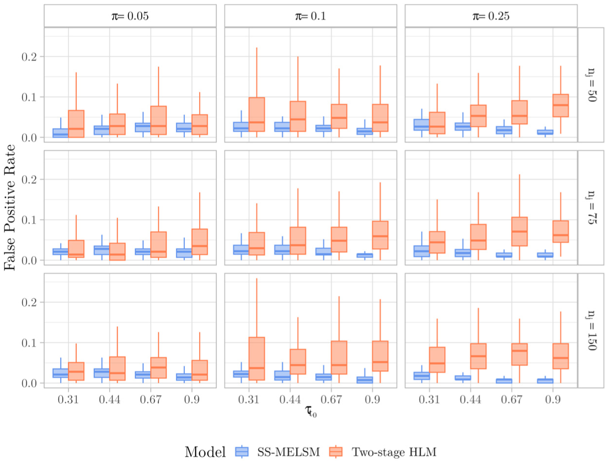
False Positive Rate values across simulations, including 150 schools.
The trade-off between the two methods is best resolved by the F1 score, which balances sensitivity and precision. As summarized in Figure 2, the results favor the SS-MELSM, which demonstrated a superior F1 score in challenging conditions with small effect sizes (e.g. scores of 0.55 vs. 0.48) as well as favorable conditions with larger samples and effect sizes.
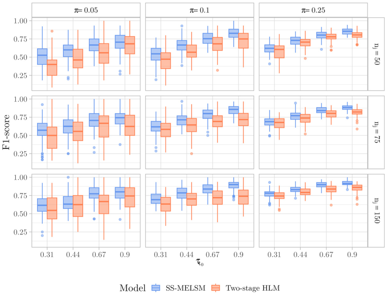
F1-score values across simulations, including 150 schools.
Finally, we also addressed one reviewer’s concern about differences between HLM and SS-MELSM being driven by the direction of the variability (i.e. unusually high or low). A small-scale simulation study, included in our OSF repository, shows that both methods’ sensitivity performance generally does not depend on the direction of residual deviations. Additionally, we found a greater tendency for two-stage HLM to produce false positives when classifying schools as unusually consistent, compared to a more balanced specificity from SS-MELSM in both directions of the effect.
Secondary Simulation: Small and Unbalanced Samples
An important contribution of Raudenbush and Bryk (1987) transformation is its ability to account for degrees of freedom, which is especially relevant in small-sample contexts. To assess performance in these more challenging scenarios, we conducted a secondary simulation with 20 and 50 schools and smaller, unbalanced school sizes of 10 and 30 on average.
In terms of classification, both methods performed similarly with respect to sensitivity. However, mirroring the results of the primary study, the two-stage HLM had significantly higher and more variable false positive rates. Regarding parameter recovery, the two-stage HLM showed near-zero bias when no true effects existed. However, when there were atypical schools in the sample, the SS-MELSM’s estimates were, on average, much closer to the true value, demonstrating a clear advantage when effects are present. Detailed results of the secondary simulation study can be found in https://osf.io/w2r98/files/wfnsk.
Summary of Findings
Our simulations showed that SS-MELSM can recover true signals with good specificity. Across conditions, SS-MELSM was especially effective at finding true signals while erring on the side of caution. The two-stage HLM sometimes showed higher sensitivity, but this was accompanied by lower specificity and more false positives. The SS-MELSM approach may miss some true positives, but it is substantially better and more consistent at avoiding misclassification. Overall, we found support for using SS-MELSM as a cautious yet reliable tool for identifying clusters with unusual variability.
Illustrative Example
Building on the results of the simulation study, we next demonstrate the model’s practical utility by applying it to a real-world education dataset. Our goal in this section is to show how SS-MELSM can be used to identify schools whose students are unusually inconsistent (or consistent) in their math achievement, even after accounting for school- and student-level predictors. The proposed model estimates fixed and random intercepts for both location and scale and adds SES as a covariate. We also use this empirical data to briefly illustrate the model comparison approach employed by
Subjects and Procedure
We use data from The Elementary Education Evaluation System (Saeb), an assessment program conducted by the Brazilian government (Instituto Nacional de Estudos e Pesquisas Educacionais Anísio Teixeira, 2021). Saeb is designed to evaluate the quality of elementary education across Brazil by administering standardized tests and questionnaires to students in public schools and a representative sample of private schools every 2 years. Student scores are reported on the Saeb unified scale, standardized in the reference population to have a mean of 0 and an SD of 1. For this study, we analyze a subset of 11,386 11th- and 12th-grade students from 160 randomly selected schools in the state of Rio de Janeiro who took the 2021 exam. We limited the sample to a single state to avoid potential differences arising from variations in educational systems across states. Additionally, the reduced sample size allows the inclusion of this dataset in the
In this subsample, school sizes ranged from 1 to 493 students, with a mean of 71.2 (SD = 74.5). The schools were nearly all public (99.4%) and located in urban areas (95.2%). Mathematics achievement had a mean of 0.15 (SD = 0.85), ranging from 1.82 to 3.23. Student SES averaged 4.94 (SD = 0.81), ranging from 2.20 to 7.62. Saeb computes SES based on parental education, household assets, and purchased services, scaling it in the reference population to a mean of 5 and SD of 1.
Statistical Analyses
To identify schools with unusual achievement consistency, we specified and compared three SS-MELSMs of increasing complexity. Model 1 served as an intercept-only baseline, Model 2 added fixed effects for SES, and Model 3 extended the model with a random slope for student-level SES.
Model 1: Intercept-Only Model
This baseline model estimates the average math achievement and the average within-school variability across all schools, including random intercepts for both the location (u0j) and scale (t0j) components to account for school-level differences. The model is specified as shown in Equation (20) from the simulation study.
Model 2: Covariate Model
This model extends the baseline by adding student- and school-level SES as predictors in both the location and scale submodels. The likelihood is defined as:
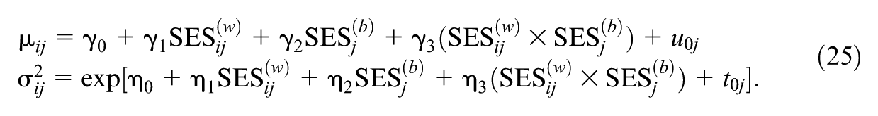
The fixed effects
Model 3: Random-Slope Model
The final model builds on Model 2 by adding a random slope for student-level SES (t1j) to the scale component. This allows the effect of a student’s relative SES on their achievement consistency to vary from school to school. The scale submodel is thus defined as:

Across Models 2 and 3, the SES predictor was partitioned to disentangle the within-school effect (
All models included random intercepts for location (u0j) and scale (t0j), with a spike-and-slab prior placed on the scale random effect. Priors were consistent with those defined in the Simulation Study.
Model Fit and Model Comparison
All models were fit with six chains of 3,000 iterations and 12,000 warm-up samples (example code is provided in https://github.com/consistentlyBetter/ivd). The number of iterations was chosen to ensure good quality of the parameter estimates, with the models converging as indicated by potential scale reduction factors
We compared the predictive accuracy of the estimated models using Pareto smoothed importance sampling leave-one-out cross-validation (PSIS-LOO), reporting both the expected log pointwise predictive density (
Note that the SS-MELSM is a single joint model in which all random effects are estimated simultaneously under the spike-and-slab prior. Therefore, the model fit statistics reported here, such as PSIS-LOO, assess the overall predictive accuracy of this single, integrated model structure.
Results
We fit three competing SS-MELSMs to the data and compared their predictive accuracy using PSIS-LOO to determine the best-fitting model. The models included a baseline intercept-only model (Model 1), a model with SES covariates (Model 2), and a model that added a random slope for student-level SES to the scale component (Model 3).
The model comparison results showed that Model 2 provided a substantially better fit than the intercept-only Model 1 (
In Model 2, both student-level (
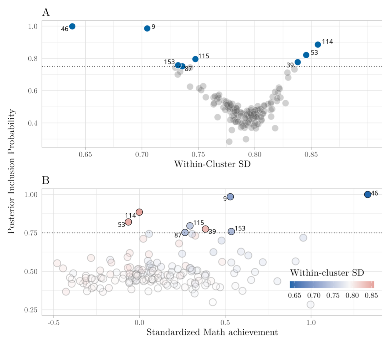
The primary goal of the analysis was to identify schools with atypical achievement consistency. Using the PIP > 0.75 criterion, the SS-MELSM flagged eight schools in Model 2. As shown in Figure 3, Panel A, these schools represent both extremes of the consistency spectrum. Five flagged schools exhibited unusually high consistency (a smaller-than-average residual SD), while three exhibited unusually low consistency (a larger-than-average residual SD). Panel B of Figure 3 shows that some of the most consistent schools were also among the highest achieving: school 46 was not only highly consistent in math achievement but also performed better than the average in our sample. We can also observe a mix of more inconsistent and consistent schools within 0.5 standard deviations of the estimated mean. These findings are not unexpected, as there is a negative correlation between mean and variance (high-achieving schools tend to have smaller variance). Still, some schools closer to the average showed both high and low within-cluster variance. This lends some support to the idea that average performance and consistency of performance can be distinct features of a school. The SS-MELSM can identify schools that are outliers on this latter dimension, even after accounting for covariates such as SES.
Scatter plots of PIP for the scale random intercept.
It appears that the model’s decision to flag a school was driven by both the school’s size and the weight of SES. A modest deviation from the average in a large school, like 115 (
Discussion
In this paper, we introduced the SS-MELSM, an extension of the standard MELSM, to identify clusters with unusual within-cluster variability. The motivation for this work is rooted in the growing body of literature suggesting that variability in academic achievement reflects elements that go unaccounted for when focusing on the mean performance. As such, the modeling framework presented here could serve policymakers and other stakeholders in identifying schools or school classes that are subject to factors such as SES or resource use, which exacerbate or mitigate differences in student achievement. From a policy perspective, reducing variability in achievement does not usually mean lowering high performance and raising low performance to meet in the middle. More often, the goal is to raise all students’ achievement levels, thereby reducing disparities while increasing the mean.
The statistical framework presented in this study incorporates both mean and variance, enabling policymakers to evaluate interventions with greater nuance. For example, interventions that provide more resources or support to students who need it most can reduce differences within a school and also raise overall performance. Conversely, recognizing situations where low variability corresponds to uniformly low performance is equally important for informed policy decisions.
Methodologically, the SS-MELSM builds upon the foundation laid by Hedeker et al. (2008), who introduced a framework for simultaneously modeling cluster-specific means and variances, with variance submodels depending on covariates. This one-stage approach stands in contrast to two-stage methods for modeling dispersion (Raudenbush & Bryk, 1987). While two-stage models are well established, they introduce an implicit assumption about the independence of location and scale random effects that is not present in our approach. Specifically, the main difference between an MELSM model and the two-stage approach is that in the MELSM, the covariance matrix (and thus the correlation matrix) of all random effects across location and scale is estimated jointly within the likelihood (see Equation 6). In two-step approaches, these correlations do not exist during estimation, implying perfect orthogonality among location and scale random effects. While it is possible to compute their empirical correlation after estimating each step, this correlation plays no role in model fitting. In contrast, given the joint model of the MELSM, dependencies between location and scale can influence all other parameters during estimation – this is a general advantage of joint models (Wolfinger & Tobias, 1998).
As noted by Leckie et al. (2014), this approach yields more precise variance estimates in the scale model. Simulation results available in the OSF repository further demonstrate this benefit, as the correlation between schools’ deviations from the mean and their variability is, on average, underestimated when employing a two-stage approach.
By incorporating a spike-and-slab prior into the scale component, the SS-MELSM provides probabilistic measures of random-effect inclusion via PIPs and Bayes factors. In contrast to traditional MLM, which assumes all random effects are relevant, this method selectively differentiates between meaningful and negligible random components. This helps make informed decisions about whether a school demonstrates unusually consistent or inconsistent achievement, thereby highlighting clusters where differences in variability may be due to factors such as teaching quality, student engagement, or available resources.
Our simulation study gave further support for the SS-MELSM. Compared with the two-stage V-known HLM approach (Raudenbush & Bryk, 1987), the SS-MELSM had higher specificity and better control of false positives, while matching or exceeding overall accuracy using the F1 score. In cases where no schools differed in variability, the two-stage method still identified some schools as atypical, whereas the SS-MELSM showed almost perfect specificity. This means the SS-MELSM is less susceptible to over-interpreting natural extremes and is more reliable at finding truly unusual patterns. It is important to remember that while screening often focuses on sensitivity to avoid missing cases, this approach only works well when follow-up costs are low. In education policy, a model with high sensitivity but low precision could lead to too many referrals for further study, potentially overwhelming the system it is intended to support (VanMeveren et al., 2020).
Having established the SS-MELSM’s performance in simulation, we next applied it to data from the Brazilian Evaluation System of Elementary Education (Saeb), a large-scale educational assessment. The Saeb application illustrated how the SS-MELSM provides insights beyond mean scores, showing that higher-achieving schools were also more consistent. The model identified 8 of 160 schools with unusual variability, even after accounting for SES differences. The inclusion of SES improved the model’s predictive accuracy, as evidenced by the PSIS-LOO model comparison, which favored Model 2 over Model 1. This finding aligns with existing research highlighting the significant role of SES in academic achievement (Davis-Kean, 2005; Davis-Kean et al., 2021; Sirin, 2005).
Despite the promising results of SS-MELSM, several limitations should be acknowledged. First, estimating the SS-MELSM can be computationally demanding, particularly for models with many random effects. While the
The models discussed, especially those with multiple random effects, involve many parameters, raising questions about necessary sample sizes and observations per cluster. While simpler MELSMs can be estimated with relatively few data points (Leckie et al., 2014; Walters et al., 2018), increased complexity demands more data. While broad, our simulation was designed to compare the relative performance of the models, not as a formal power analysis to establish minimum sample size requirements for a given effect, and a proper investigation of data needs is still lacking.
In our simulation, the fitted model correctly matched the data-generating process, which is often not the case in applied research. A key limitation is that we did not test the consequences of omitting an important covariate that influences both the mean and the variance. Such a model misspecification could bias the estimates of the random effects and potentially inflate the perceived heterogeneity. Furthermore, we generated data from a normal distribution, and the performance of the tested methods might be different if the underlying student-level data were skewed or heavy-tailed.
Finally, we used a standard set of priors and a common threshold for classification. While these are justified by convention, a formal sensitivity analysis was not conducted to determine how different prior specifications might affect the results.
In conclusion, the SS-MELSM offers a valuable extension to the MELSM framework. By jointly modeling the mean and variance components and incorporating a principled method for random effect selection, it offers a deeper understanding of academic achievement. By moving beyond simple averages, researchers and educators can use the SS-MELSM to identify and support educational environments that help students achieve well and do so consistently.
Supplemental Material
sj-pdf-1-jeb-10.3102_10769986261426004 – Supplemental material for Beyond Average Scores: Identification of Consistent and Inconsistent Academic Achievement in Grouping Units
Supplemental material, sj-pdf-1-jeb-10.3102_10769986261426004 for Beyond Average Scores: Identification of Consistent and Inconsistent Academic Achievement in Grouping Units by Marwin Carmo, Donald Williams and Philippe Rast in Journal of Educational and Behavioral Statistics
Footnotes
Declaration of Conflicting Interests
The authors declared no potential conflicts of interest with respect to the research, authorship, and/or publication of this article.
Funding
The authors disclosed receipt of the following financial support for the research, authorship, and/or publication of this article: The work reported in this publication was partially supported by an award to PR from the Learning Engineering Tools Competition, organized by The Learning Agency LLC. The content is solely the responsibility of the authors and does not necessarily represent the official views of the funding agencies.
Notes
Authors
MARWIN CARMO is a PhD student at the University of California, Davis, 135 Young Hall One Shields Avenue, Davis, CA 95616; e-mail:
DONALD WILLIAMS is a PhD in psychology from the University of California, Davis, 135 Young Hall One Shields Avenue, Davis, CA 95616; e-mail:
PHILIPPE RAST is a professor at the University of California, Davis, 135 Young Hall One Shields Avenue, Davis, CA 95616; e-mail:
References
Supplementary Material
Please find the following supplemental material available below.
For Open Access articles published under a Creative Commons License, all supplemental material carries the same license as the article it is associated with.
For non-Open Access articles published, all supplemental material carries a non-exclusive license, and permission requests for re-use of supplemental material or any part of supplemental material shall be sent directly to the copyright owner as specified in the copyright notice associated with the article.