Sage Journals: Discover world-class research

Abstract

The traditional approach to estimating the consistency of school effects across subject areas and the stability of school effects across time is to fit separate value-added multilevel models to each subject or cohort and to correlate the resulting empirical Bayes predictions. We show that this gives biased correlations and these biases cannot be avoided by simply correlating “unshruken” or “reflated” versions of these predicted random effects. In contrast, we show that fitting a joint value-added multilevel multivariate response model simultaneously to all subjects or cohorts directly gives unbiased estimates of the correlations of interest. There is no need to correlate the resulting empirical Bayes predictions and indeed we show that this should again be avoided as the resulting correlations are also biased. We illustrate our arguments with separate applications to measuring the consistency and stability of school effects in primary and secondary school settings. However, our arguments apply more generally to other areas of application where researchers routinely interpret correlations between predicted random effects rather than estimating and interpreting these correlation directly.

Keywords

multilevel model multivariate response school effects consistency stability value-added

1. Introduction

There are now many studies that investigate the effects of individual schools on student achievement using multilevel value-added analyses (see the handbooks by Teddlie & Reynolds, 2000, and Townsend, 2007, the recent review by Reynolds et al., 2014, and the 2004 special issue of the Journal of Educational and Behavioral Statistics devoted to value-added models, Wainer, 2004). At their simplest, these analyses use two-level students within-schools random-intercept models to regress student achievement at the end of the value-added period of interest on student achievement at the start of the period (Goldstein, 1997). Further adjustments are usually made for student demographic and socioeconomic characteristics deemed beyond the control of the school (Raudenbush & Willms, 1995). Individual school effects are then calculated postestimation as empirical Bayes predictions (i.e., “shrinkage” estimates) of the random-intercept effects. While our focus is on random-effects models (multilevel or hierarchical linear models), we note that value-added models are also often implemented in the research literature and various school accountability systems as fixed-effects models or as linear regression models where the student residuals are averaged up to the school-level postestimation. We refer the reader to Guarino, Reckase, and Wooldridge (2015) for a recent discussion of these and other estimators.

Two fundamental issues in this field are “the consistency of school effects across subject areas” and “the stability of school effects across time” (Teddlie & Reynolds, 2000; Townsend, 2007). Interest lies in establishing the extent to which effectiveness is an overall phenomenon versus a subject-specific phenomenon and the extent to which school effects persist over successive cohorts of students. The less consistent school effects are across subjects, the more important it is to study them in their own right as opposed to just overall achievement. The less stable school effects are over time, the less reliable published school effects will be as a guide for school choice (Leckie & Goldstein, 2009). Schools may exhibit inconsistent school effects due to differences across subjects in teacher effectiveness or in how schools concentrate their limited financial resources. Schools may exhibit unstable school effects due to changes from one cohort to the next in school policies, leadership, staff turnover, and teaching methods and materials. In a recent review, Reynolds et al. (2014) summarize most studies as reporting moderately positive correlations between school effects across subjects but higher correlations between school effects for consecutive cohorts. Thus, while schools are to some extent differentially effective across different subject areas, school effects tend to be relatively stable in most subjects at least across the short term. While our focus is on school effects, we note that the notions of consistency and stability also apply to teacher effects, and this literature is well summarized by the recent review by Loeb and Candelaria (2012).

The traditional approach to estimating consistency and stability correlations is to fit separate value-added models to each subject or cohort and to correlate empirical Bayes predictions of the school effects across these models. This separate modeling approach appears problematic. First, fitting separate models is equivalent to fitting a joint (multivariate response) value-added model where we treat the subject- or cohort-specific school effects (and student residuals) as independent of one another, rather than correlated, implying that the “true” consistency or stability correlation in the population is zero. Second, the empirical Bayes predictions, whether from separate or joint models, are shrinkage estimates whose variances and correlations typically differ from those implied by the model parameters. It therefore seems very likely that the consistency and stability correlations that result from this approach will be biased. There appears, however, to be a lack of awareness of this problem as demonstrated by the large number of studies that apply this approach unreservedly (e.g., Braun & Wainer, 2007; Dumay, Coe, & Anumendem, 2014; Gorard, Hordosy, & Siddiqui, 2013; Luyten, 1998; Marks, 2015; Newton et al., 2010; Perry, 2016; Shavelson et al., 2016; Wilson & Piebalga, 2008).

The preferred approach to estimating the consistency and stability of school effects is to fit a joint value-added model to all subjects or cohorts under investigation which, rather than treat the school effects as independent, allows them to be correlated and directly estimates these correlations as model parameters. This joint modeling approach avoids the biases introduced when correlating empirical Bayes predictions from separate models. While a number of papers have followed this second approach (e.g., Doolaard, 2002; Goldstein et al., 1993; Grilli, Pennoniy, Rampichini, & Romeoy, 2016; Leckie & Goldstein, 2009, 2011; Ma, 2001; Willms & Raudenbush, 1989), none of them indicate that a reason for doing so is to avoid the biased correlations that arise from the separate modeling approach. Instead, these papers motivate their use of joint models by referring to their other notable advantages such as the ability to conduct cross-equation hypothesis tests to study differential influences of student characteristics across subjects or cohorts. It therefore appears that the biases associated with the separate modeling approach are not widely understood, even among those who already fit joint models.

We are only aware of one study that explicitly states that the correlations they report between empirical Bayes predictions from separately fitted models are biased (Thomas, Sammons, Mortimore, & Smees, 1997). The authors, who study the consistency of school effects across seven different academic subjects, reporting correlations in the range .20 to .72 (see their Table 5), state that their correlations are biased upward (p. 188):

It is important to point out that any correlations between school value added scores (i.e., residuals) may be viewed as technically “inflated” estimates due to the fact that there is an element of “shrinkage” (towards the overall mean score) in the calculation of these scores, particularly for schools with very small number of pupils.

This statement suggests that had the authors correlated unshrunken versions of their empirical Bayes predictions they would have recovered unbiased correlations. (We will show that this is not actually the case.) They do not, however, go on to report these correlations. However, given the above discussion, shrinkage is not the only source of bias in the separate modeling approach. The more fundamental problem is that by fitting separate models the authors implicitly assume that schools have independent effects across subjects (and similarly that students’ performances within their schools are unrelated across subjects).

In a subsequent article, this time on studying the stability of school effects across 10 cohorts of students, Thomas, Peng, and Gray (2007) do fit a joint model. However, rather than reporting correlations estimated directly from the model parameters, they again report correlations between empirical Bayes prediction of the school effects (see their Table 5). These correlations lie between .78 and .89 for adjacent years, .62 and .68 for 10 years apart, and .62 for 10 years apart. It is not clear why they follow this approach, especially as they acknowledge that these correlations are also biased (p. 277):

Due to shrinkage the correlations between model residuals…are slightly stronger than the “true” correlations estimated by the analysis.

They indicate that the upward biases in their study are slight, but they do not quantify how slight. The authors again suggest that the cause of this bias is shrinkage, but again they do not report the corresponding correlations between unshrunken versions of their empirical Bayes predictions to show this.

A separate concern with the random-effect models discussed so far, whether separately or jointly estimated, is that they assume that there is no school-level confounding (the covariates are assumed uncorrelated with the school effects). This assumption will fail if, for example, students with high prior achievement systematically select into more effective schools. This will lead to biased parameter estimates and biased predictions of the school effects. Where these biases are nontrivial, one potential solution is to use fixed- rather than random-effects models, as they allow for school-level confounding. Another solution, proposed by Castellano, Rabe-Hesketh, and Skrondal (2014), is to use Hausman–Taylor random-effects models that have the notable advantage over fixed-effects models of being able to estimate the effects of school- as well as student-level covariates.

The purpose of this article is to explore and clarify the biases associated with correlating predicted school effects from value-added models for the purpose of estimating the consistency and stability of school effects. We consider correlations between “unshrunken” and “reflated” estimates of the school effects as well as the usual shrunken empirical Bayes predictions. We study the different form these biases take depending on whether the predicted school effects are derived from separate models fitted to each subject or cohort as opposed to when they are derived from a joint model. We argue that all these biases can be avoided by simply calculating the consistency and stability correlations directly from the model parameters of the joint model.

The article proceeds as follows. In Section 2, we introduce the separate and joint modeling approaches. In Section 3, we present the biases associated with correlating predicted school effects derived from each approach. In Section 4, we illustrate our arguments with two separate applications to English schools data, first measuring the consistency of primary school effects across English and mathematics in 2014 and second measuring the stability of secondary school effects on student overall achievement between 2013 and 2014. We end with a short conclusion and a discussion of the wider implications of our findings to other areas of application where researchers routinely interpret correlations between predicted random effects rather than estimating and interpreting these correlation directly.

2. Separate and Joint Models

We first present the traditional separate modeling approach to estimating the consistency and stability of school effects. We then present the joint modeling approach. For simplicity, and for each approach, we consider in detail the case of studying the consistency of school effects across two subject areas for a single cohort. We then briefly describe how estimating the stability of school effects in a single subject area but across two cohorts differs from this. Lastly, we explain how each approach can be extended to more general settings with multiple subjects or cohorts.

While we focus on the most standard data designs for estimating the consistency and stability of school effects, we note that other designs are possible where, for example, students within each school study only one of the subjects and therefore contribute only one achievement score each, or where a single cohort of students is tracked across multiple value-added periods and interest lies in correlating the school effects across these value-added periods. See Section S3 of the online Supplemental Material for how these alternative data designs imply changes to the presented models and biases.

2.1. The Separate Modeling Approach: Correlate Empirical Bayes Predictions From Separately Fitted Models

Let y_ij denote the achievement score at the end of the value-added period of interest in a given subject for student i ( $i = 1, \dots, n_{j}$ ) in school j ( $j = 1, \dots, J$ ). The two-level random-intercept model (Goldstein, 2011; Raudenbush & Bryk, 2002; Skrondal & Rabe-Hesketh, 2004; Snijders & Bosker, 2012) for y_ij can then be written as

y_{i j} = x_{i j}^{′} β + u_{j} + e_{i j},

where x _ij is the vector of student- and potentially school-level covariates (i.e., student prior achievement at the beginning of the value-added period as well as other student demographic and socioeconomic characteristics) with regression coefficients β, u_j is the school random intercept effect (i.e., value-added school effect), and e_ij is the student residual. The school effects and student residuals are assumed to have zero means and constant variances $σ_{u}^{2} and σ_{e}^{2}$ and to be independent across levels and independent of the covariates. The intraclass correlation coefficient (ICC), calculated as $σ_{u}^{2} {(σ_{u}^{2} + σ_{e}^{2})}^{- 1}$ and interpreted as the expected correlation between two students’ conditional scores, in this context, is also used to quantify the “size of the school effects,” in other words, the relative importance of schools as a source of variation in student value added.

While the above random-effects model is applied routinely in the literature, a general concern with this class of model is that it assumes the covariates are uncorrelated with the cluster effects. This assumption will fail in the current setting if, for example, students with higher prior achievement systematically select into more effective schools. The regression coefficient on prior achievement would then be biased upward that would in turn bias the estimated school effects toward zero (e.g., Castellano, Rabe-Hesketh, & Skrondal, 2014). When the value-added model includes no school-level covariates, a popular solution is to refit the model as a fixed-effects model since this approach will estimate unbiased regression coefficients and therefore school effects irrespective of whether the student-level covariates correlate with the school effects. In practice, however, fixed- and random-effects implementations of school value-added models often give very similar results, and this is what we also see in our two applications. We note that this contrasts application of these models to individual-year panel data and other settings where more pronounced differences are often seen due to the greater degree of clustering typically exhibited by the covariates as well as the considerably smaller size of clusters.

When value-added models additionally include school-level covariates, the fixed-effects model cannot be used as the inclusion of school dummy variables to estimate the school effects precludes the introduction of school-level covariates. Castellano et al. (2014), however, show how the Hausman–Taylor random-effects model developed for panel data can be innovatively applied in this setting to estimate school effects adjusted for both the student- and school-level covariates. An advantage of this approach is that it can, at least in principle, also be applied when the school-level covariates are themselves correlated with the school effects. School mean prior achievement, for example, is sometimes included to capture a potential positive effect of being educated among higher achieving peers but is likely to be endogenous for the reason given earlier. However, as explained by Castellano et al. (2014), the value-added model must now include at least as many exogenous student-level covariates, as there are endogenous school-level covariates and this may often not be the case. We shall not consider school-level covariates further in this article.

Without wishing to diminish the importance of this debate, we note that whatever the chosen covariates and argued plausibility or not of the model assumptions, correlating predicted school effects, whether from separate or joint models, will give different correlations to those estimated directly by the joint model. Thus, our interest here is not in exploring how and why different value-added model specifications produce different estimates of the school effects, rather it is in revealing and explaining why competing approaches for correlating the school effects will give different results for any given value-added model. We return to the importance of correct model specification and assumptions in the discussion.

Having fitted the model, values are assigned to the school effects via empirical Bayes prediction. Empirical Bayes predictions additionally assume the school effects are normally distributed, though we note that in linear models this assumption is not required when one alternatively derives these predictions as estimated best linear unbiased predictions (Henderson, 1950; Skrondal & Rabe-Hesketh, 2009). The empirical Bayes predictor is

{\tilde{u}}_{j}^{EB} = {\hat{R}}_{j} {\frac{1}{n_{j}} \sum_{i = 1}^{n_{j}} (y_{i j} - x_{i j}^{′} \hat{β})} where 0 < {\hat{R}}_{j} \equiv \frac{{\hat{σ}}_{u}^{2}}{{\hat{σ}}_{u}^{2} + {\hat{σ}}_{e}^{2} / n_{j}} < 1.

The term in curly brackets is the school mean of the estimated “raw” or total student residuals for school j and is often called the maximum likelihood estimate of u_j . ${\hat{R}}_{j}$ is a shrinkage factor that pulls the empirical Bayes prediction toward 0, the population average. Thus, the empirical Bayes predictions and the maximum likelihood estimates are often referred to as “shrunken” and unshrunken estimates of the school effects. The shrinkage factor is the reliability of the school means as a measurement of u_j and is defined as the estimated variance of the school effects divided by the estimated variance of the school means. The reliability increases when ${\hat{σ}}_{u}^{2}$ increases relative to ${\hat{σ}}_{e}^{2}$ and as $n_{j} \to \infty$ . Thus, the empirical Bayes predictions are shrunk less the more clustering there is in the data (i.e., the larger the size of the school effects) and are shrunk less for large schools than small schools.

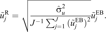
While the variance of the shrunken estimates is less than the variance of the unshrunken estimates, neither of these variances match the model-based estimate of the school variance, which lies between the two (see Table A1 in the Appendix). A third set of estimates sometimes calculated are therefore so-called reflated empirical Bayes predictions, which are simply the empirical Bayes predictions rescaled so that their variance equals the model-based estimate (Carpenter, Goldstein, & Rasbash, 2003):

{\tilde{u}}_{j}^{R} = \sqrt{\frac{{\hat{σ}}_{u}^{2}}{J^{- 1} \sum_{j = 1}^{J} {({\tilde{u}}_{j}^{EB})}^{2}}} {\tilde{u}}_{j}^{EB} .

Fitting Equation 1 separately to achievement scores in each subject results in two sets of empirical Bayes predictions, ${\tilde{u}}_{1 j}^{EB} and {\tilde{u}}_{2 j}^{EB}$ . In the separate modeling approach, the correlation between these predictions is then reported as a measure of the consistency of the school effects across subjects. If we instead wish to estimate the stability of school effects in a single subject area but across two cohorts, we simply fit Equation 1 separately to the two cohorts of students and again correlate the resulting empirical Bayes predictions. When there are multiple subjects or cohorts, additional models are fitted leading to further sets of empirical Bayes predictions and multiple consistency or stability correlations.

2.2. The Joint Modeling Approach: Estimate the Correlations Directly From the Model Parameters

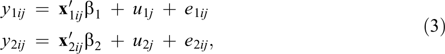
Let $y_{1 i j} and y_{2 i j}$ denote the achievement scores in academic subject 1 and 2 for student i ( $i = 1, \dots, n_{j}$ ) in school j ( $j = 1, \dots, J$ ). The model can then be written as

\begin{array}{l} y_{1 i j} = x_{1 i j}^{′} β_{1} + u_{1 j} + e_{1 i j} \\ y_{2 i j} = x_{2 i j}^{′} β_{2} + u_{2 j} + e_{2 i j}, \end{array}

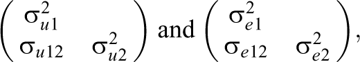
where the subject-specific school random intercept effects $u_{1 j} and u_{2 j}$ and student residuals have bivariate distributions assumed to have zero means and covariance matrices

(\begin{matrix} σ_{u 1}^{2} \\ σ_{u 12} & σ_{u 2}^{2} \end{matrix}) and (\begin{matrix} σ_{e 1}^{2} \\ σ_{e 12} & σ_{e 2}^{2} \end{matrix}),

respectively. These bivariate distributions are often assumed to be bivariate normal, although this is not required for consistent estimation of the parameters and standard errors.

The ICC is now defined separately for each subject, $σ_{u 1}^{2} {(σ_{u 1}^{2} + σ_{e 1}^{2})}^{- 1} and σ_{u 2}^{2} {(σ_{u 2}^{2} + σ_{e 2}^{2})}^{- 1}$ allowing schools to differ in their importance across subjects. While not our focus here, we note that the joint model allows two further correlations of interest. First, the expected correlation between a student’s conditional score in each subject $(σ_{u 12} + σ_{e 12}) {(σ_{u 1}^{2} + σ_{e 1}^{2})}^{- .5} {(σ_{u 2}^{2} + σ_{e 2}^{2})}^{- .5}$ . Second, the expected correlation between two students’ conditional scores in two different subjects $σ_{u 12} {(σ_{u 1}^{2} + σ_{e 1}^{2})}^{- .5} {(σ_{u 2}^{2} + σ_{e 2}^{2})}^{- .5}$ . Of these, the first is perhaps the more interesting allowing researchers to answer the question, “To what extent do students who score higher than predicted in one subject also score higher than predicted in the second subject?”

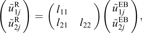
The consistency correlation is now estimated directly as function of the model parameters, $ρ_{u 12} = σ_{u 12} σ_{u 1}^{- 1} σ_{u 2}^{- 1}$ . The correlation between the student residuals is similarly defined as $ρ_{e 12} = σ_{e 12} σ_{e 1}^{- 1} σ_{e 2}^{- 1}$ .

While no longer needed for estimating the consistency of school effects, the empirical Bayes predictions of the school effects in each subject may still be desired for the purpose of making statements about individual schools. These are calculated as Skrondal and Rabe-Hesketh (2004, section 7.6):

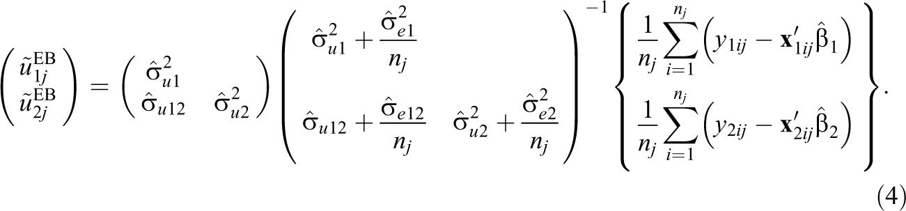
(\begin{matrix} {\tilde{u}}_{1 j}^{EB} \\ {\tilde{u}}_{2 j}^{EB} \end{matrix}) = (\begin{matrix} {\hat{σ}}_{u 1}^{2} \\ {\hat{σ}}_{u 12} & {\hat{σ}}_{u 2}^{2} \end{matrix}) {(\begin{matrix} {\hat{σ}}_{u 1}^{2} + \frac{{\hat{σ}}_{e 1}^{2}}{n_{j}} \\ {\hat{σ}}_{u 12} + \frac{{\hat{σ}}_{e 12}}{n_{j}} & {\hat{σ}}_{u 2}^{2} + \frac{{\hat{σ}}_{e 2}^{2}}{n_{j}} \end{matrix})}^{- 1} {\begin{matrix} \frac{1}{n_{j}} \sum_{i = 1}^{n_{j}} (y_{1 i j} - x_{1 i j}^{′} {\hat{β}}_{1}) \\ \frac{1}{n_{j}} \sum_{i = 1}^{n_{j}} (y_{2 i j} - x_{2 i j}^{′} {\hat{β}}_{2}) \end{matrix}} .

Here, the shrinkage factor is now a shrinkage matrix defined as the multiplication of the first two matrices. Thus, the empirical Bayes predictions for each subject is now influenced by the mean total residual in the other subject as well as by its own mean total residual. That is, the empirical Bayes predictions are shrunk toward one another as well as toward the overall mean in each subject.

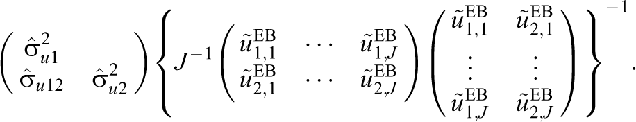
The corresponding unshrunken or maximum likelihood estimates are given by the final vector in Equation 4, while the reflated empirical Bayes predictions (whose variances and covariance are increased to equal the model-based estimates, Carpenter et al., 2003) are given by

(\begin{matrix} {\tilde{u}}_{1 j}^{R} \\ {\tilde{u}}_{2 j}^{R} \end{matrix}) = (\begin{matrix} l_{11} \\ l_{21} & l_{22} \end{matrix}) (\begin{matrix} {\tilde{u}}_{1 j}^{EB} \\ {\tilde{u}}_{2 j}^{EB} \end{matrix}),

where the first matrix after the equals sign is the Cholesky factor of

(\begin{matrix} {\hat{σ}}_{u 1}^{2} \\ {\hat{σ}}_{u 12} & {\hat{σ}}_{u 2}^{2} \end{matrix}) {J^{- 1} (\begin{matrix} {\tilde{u}}_{1, 1}^{EB} & \dots & {\tilde{u}}_{1, J}^{EB} \\ {\tilde{u}}_{2, 1}^{EB} & \dots & {\tilde{u}}_{2, J}^{EB} \end{matrix}) (\begin{matrix} {\tilde{u}}_{1, 1}^{EB} & {\tilde{u}}_{2, 1}^{EB} \\ ⋮ & ⋮ \\ {\tilde{u}}_{1, J}^{EB} & {\tilde{u}}_{2, J}^{EB} \end{matrix})}^{- 1} .

The equivalent model for estimating the stability of school effects can be defined in a parallel fashion. However, here too, the student residual covariance σ_e12 in Equation 3 would be constrained to zero since each student is observed in only one cohort.

When there are multiple subjects or multiple cohorts, additional equations are added to the joint model (Equation 3) and the number of empirical Bayes predictions increases (Equation 4) leading to multiple consistency or stability correlations. Furthermore, we note that there is nothing to stop one simultaneously incorporating both multiple subjects and multiple cohorts into the joint model. For example, where we have student achievement scores in two subjects for two different cohorts, we can estimate a four-equation joint model with one equation for each subject cohort combination. This approach allows one to simultaneously estimate the two consistency correlations (one for each cohort) and the two stability correlations (one for each subject). There is no need to fit four separate joint models for each pairing of school effects. A notable benefit of this approach is therefore the ability to conduct inferential tests on whether the consistency correlations differ across cohorts and whether the stability correlations differ across subjects. This approach also allows one to estimate two further, albeit substantively less interesting, correlations that are the correlation between school effects relating to different subjects in different cohorts.

3. Biases

In this section, we present expressions for the expected or population correlations between the predicted school effects obtained first from the traditional separate modeling approach and then from the joint modeling approach. As in Section 2, we start by studying in detail the consistency of school effects across two subject areas for a single cohort and then proceed to briefly show how our findings differ when we study the stability of school effects in a single subject area across two cohorts. Lastly, we explain how equivalent expressions can be derived in more general settings with multiple subjects or cohorts.

We assume that the joint value-added model (Equation 3) is the true model throughout this section. For simplicity, we consider the case where each school has the same number of students n_j = n. All expressions given in this section are also shown for ease of comparison in Table A1 in the Appendix and are derived in full in the online Supplemental Material.

3.1. Correlating Predicted School Effects From Separately Fitted Models

First recognize that fitting separate models (Equation 1) to each subject achievement score is equivalent to fitting a joint model (Equation 3) to both scores but constraining $σ_{u 12} = σ_{e 12} = 0$ . (In this case, Equation 4 also simplifies to Equation 2.) Assuming Equation 3 is the true model, it can be shown (see Table A1 and online Supplemental Material) that the expected or population correlation between the empirical Bayes predictions of the school effects obtained from fitting separate models is given by

Corr ({\tilde{u}}_{1 j}^{EB}, {\tilde{u}}_{2 j}^{EB}) = \frac{σ_{u 12} + \frac{σ_{e 12}}{n}}{\sqrt{σ_{u 1}^{2} + \frac{σ_{e 1}^{2}}{n}} \sqrt{σ_{u 2}^{2} + \frac{σ_{e 2}^{2}}{n}}} .

Estimated correlations of empirical Bayes predictions will approach this quantity as the number of schools tends to infinity. The problem is that this quantity differs from the intended one, $ρ_{u 12} = σ_{u 12} σ_{u 1}^{- 1} σ_{u 2}^{- 1}$ , and so this estimator is biased and inconsistent. Equation 5 shows that the estimator is biased owing to the additional $σ_{e 12} n_{j}^{- 1}$ term in the numerator and the additional $σ_{e 1}^{2} n^{- 1} and σ_{e 2}^{2} n_{j}^{- 1}$ terms in the denominator. The magnitude of the bias therefore depends on the magnitude of the student residual variance–covariances $σ_{e 1}^{2}, σ_{e 2}^{2}, σ_{e 12}$ and school size n. Figure 1 illustrates the relationship between this estimator (y-axis) and school size (x-axis) when the true school-level correlation is .5 (denoted by the horizontal line). For simplicity, we set the ICC to be the same across the two subjects and we consider low, medium, and high clustering scenarios with ICCs equal to .05, .15, and .25, respectively (the three panels). The figure shows the estimator is biased upward when the true student-level correlation exceeds the true school-level correlation and vice versa. Thus, the estimator is pulled toward the true student-level correlation. The figure shows that the absolute magnitude of this bias reduces as school size increases and as the degree of clustering increases. See online Supplemental Material for an interactive Excel Workbook that allows one to explore how this estimator varies, as one alters the true parameter values and school size.

Figure 1.

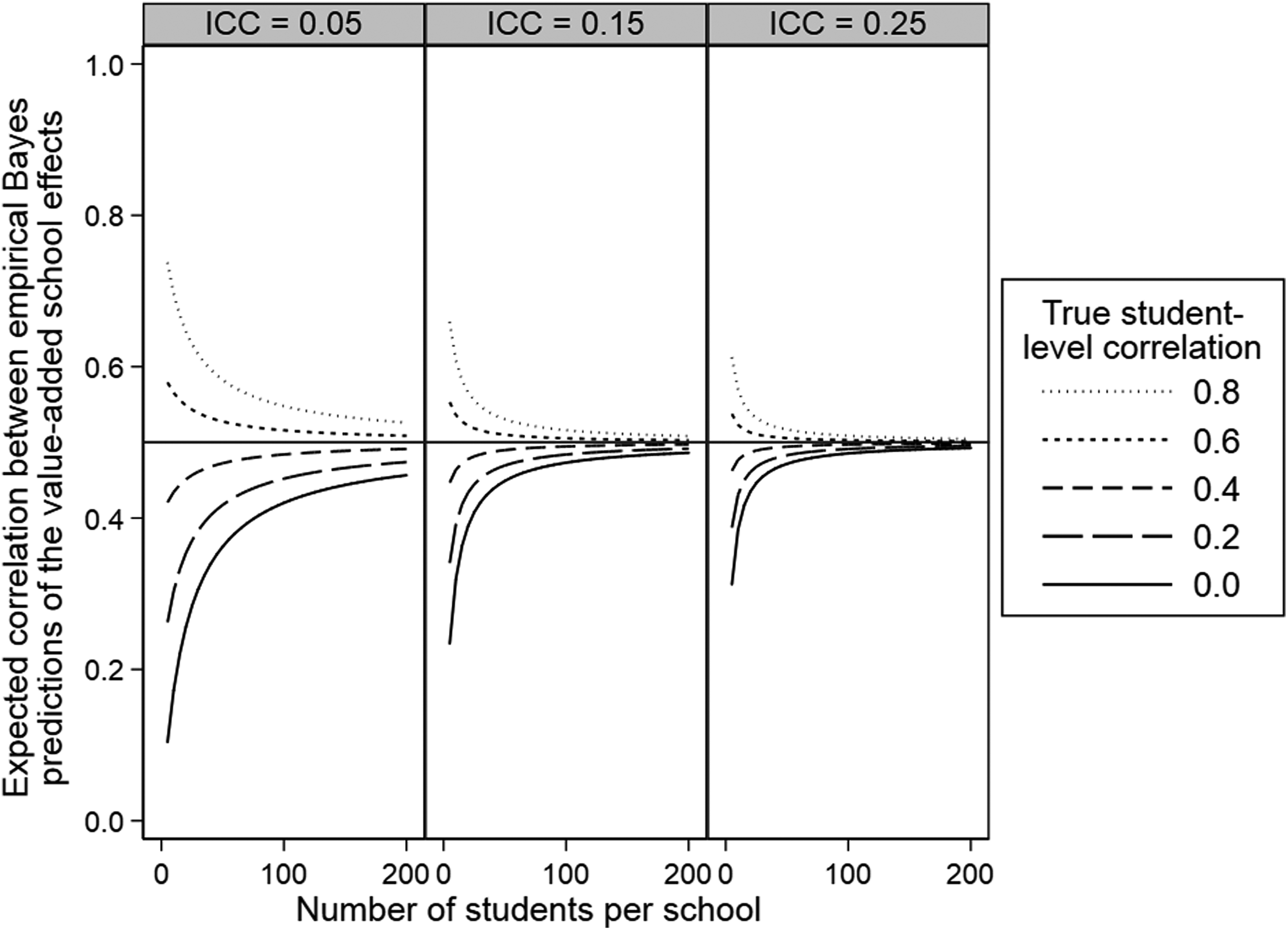
Illustration of the expected correlation between empirical Bayes predictions of the school effects derived from separate value-added models. The true school correlation is .5. ICC = intraclass correlation coefficient.

The estimator can be usefully reexpressed as

Corr ({\tilde{u}}_{1 j}^{EB}, {\tilde{u}}_{2 j}^{EB}) = \sqrt{R_{1} R_{2}} ρ_{u 12} + \sqrt{(1 - R_{1}) (1 - R_{2})} ρ_{e 12},

where R ₁ and R ₂ are the reliabilities of the maximum likelihood estimates of the school effects as measurements of $u_{1 j} and u_{2 j}$ . This formulation shows explicitly that the expected correlation between the empirical Bayes predictions is a weighted summation of two unknowns, the true school correlation ρ_u12 and the true student correlation ρ_e12. The weights lie between zero and one, and so the resulting estimator lies between $ρ_{u 12} and ρ_{e 12}$ . More weight is given to ρ_u12, as the reliability of the maximum likelihood estimates increases due to increasing clustering or school size.

Recall that Thomas, Sammons, Mortimore, and Smees (1997) in their study of the consistency of school effects across seven subject areas state that their reported correlations are inflated due to shrinkage implying that they overstate the true consistency of school effects. Our results suggest that their correlations will only be biased upward if the true student correlations across subjects exceed the true school correlations, an ordering which is unknown when one fits separate models to each subject area as these authors did. Thus, their reported correlations may equally be deflated, in which case they would understate the true consistency of school effects. Turning our attention to the explanation they give for their biased results, namely, shrinkage, our results show that this explanation is correct in that the bias (whether upward or downward) will be smaller in settings where there is less shrinkage, that is, in studies with more severe clustering and larger school sizes. Indeed, the reliabilities in Equation 6 are shrinkage factors and as these tend to one (i.e., settings with no shrinkage), the estimator tends to its true value.

It is important to realize, however, that this shrinkage explanation does not imply that simply calculating and correlating unshrunken versions of the empirical Bayes predictions (i.e., maximum likelihood estimates) provides a way to recover unbiased estimates of the true school correlations when fitting separate value-added models. Indeed, it can be shown (see Table A1 and online Supplemental Material) that the expression for the correlation between the maximum likelihood estimates of the school effects is the same as that between the empirical Bayes predictions stated in Equations 5 and 6. Essentially, while the variances and covariance between the two sets of shrunken school effects are indeed smaller than those calculated on their unshrunken counterparts, all three terms are shrunk in proportion and so the resulting correlation is the same.

In any case, the variances of the maximum likelihood estimates of the school effects are themselves upward biased estimates of the true school variances and so one would not automatically expect the correlation between them to therefore be unbiased. For this reason, some researchers may consider calculating and correlating reflated empirical Bayes predictions, as their variances and covariances equal the model-based estimates. However, in the current case of fitting separate value-added models to each subject area, there is no model-based estimate of the school covariance; the school covariance is implicitly zero. It can be shown that this transform also results in the same expression for the correlation as that between the empirical Bayes predictions (see Table A1 and online Supplemental Material). Essentially, the variances and covariance between the two sets of shrunken school effects are reflated in proportion, and so the resulting correlation is unchanged.

In terms of estimating the stability of school effects in a single subject area but across two cohorts, Equations 5 and 6 simplify as the student-level correlation is zero by definition. As a result, Figure 1 also simplifies with the only relevant lines now being the most extreme solid lines. Thus, all else equal, correlating empirical Bayes predictions from separately fitted models can be expected to lead to especially biased correlations between school effects calculated for different cohorts. The simplification of Equation 6 to $Corr ({\tilde{u}}_{1 j}^{EB}, {\tilde{u}}_{2 j}^{EB}) = \sqrt{R_{1} R_{2}} ρ_{u 12}$ is such that when rearranged the equation reveals a multiplicative correction factor $R_{1}^{- .5} R_{2}^{- .5}$ which when applied to the biased estimate recovers an unbiased estimate of the stability correlation. In practice, the number of students will vary across schools, and so this correction factor will be somewhat approximate. Nonetheless, researchers studying the stability of school effects by correlating predicted school effects from separately fitted models can now investigate and at least approximately adjust for the bias in their approach.

When there are multiple subjects or cohorts, the expected correlation between the predicted school effects relating to any two subjects or cohorts remains the same, and this is irrespective of the method of assigning values to the random effects.

3.2. Correlating Predicted School Effects From a Joint Model

Assuming again that Equation 3 is the true model, it can be shown (see Table A1 and online Supplemental Material) that the expected or population covariance matrix between the empirical Bayes predictions derived from fitting this model is given by

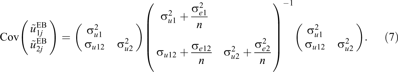
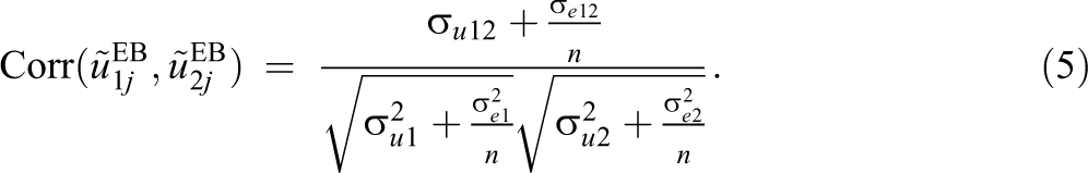
Cov (\begin{matrix} {\tilde{u}}_{1 j}^{EB} \\ {\tilde{u}}_{2 j}^{EB} \end{matrix}) = (\begin{matrix} σ_{u 1}^{2} \\ σ_{u 12} & σ_{u 2}^{2} \end{matrix}) {(\begin{matrix} σ_{u 1}^{2} + \frac{σ_{e 1}^{2}}{n} \\ σ_{u 12} + \frac{σ_{e 12}}{n} & σ_{u 2}^{2} + \frac{σ_{e 2}^{2}}{n} \end{matrix})}^{- 1} (\begin{matrix} σ_{u 1}^{2} \\ σ_{u 12} & σ_{u 2}^{2} \end{matrix}) .

The expression for the resulting correlation matrix and therefore expected correlation between ${\tilde{u}}_{1 j}^{EB} and {\tilde{u}}_{2 j}^{EB}$ can be calculated in the usual way but does not have a simple form as was the case when we fitted separate models (Equations 5 and 6). However, we can see that this estimator will also include the student residual variance–covariances $σ_{e 1}^{2}, σ_{e 2}^{2}, σ_{e 12}$ and school size n and so this approach will in general also result in biased estimates. Figure 2 illustrates the relationship between this second naive estimator (y-axis) and these factors when the true school-level correlation is again .5 (denoted by the horizontal line). The figure can be interpreted in the same way as Figure 1. The figure shows that the estimator is biased downward when the true student-level correlation exceeds the true school-level correlation and vice versa. Thus, whereas the correlation between empirical Bayes predictions derived from separately fitted models is pulled toward the true student-level correlation, the correlation between empirical Bayes predictions derived from joint models is pushed away from the true student-level correlation. As in the separate modeling approach, the figure shows that in the joint modeling approach the absolute magnitude of this bias reduces as school size increases and as the degree of clustering increases. Given that the joint model is the assumed true model, one might expect the bias associated with correlating the predicted school effects from the joint model to be less than that associated with correlating the predicted school effects from separate models. However, this is not always the case and which approach is more biased depends on the true values of the parameters in Equations 3 and 5. The more important point, however, is that both approaches produce biased correlations and these biases can be substantial. See the online Supplemental Material for an interactive Excel Workbook that allows one to explore how this estimator varies, as one alters the true parameter values and school size.

Figure 2.

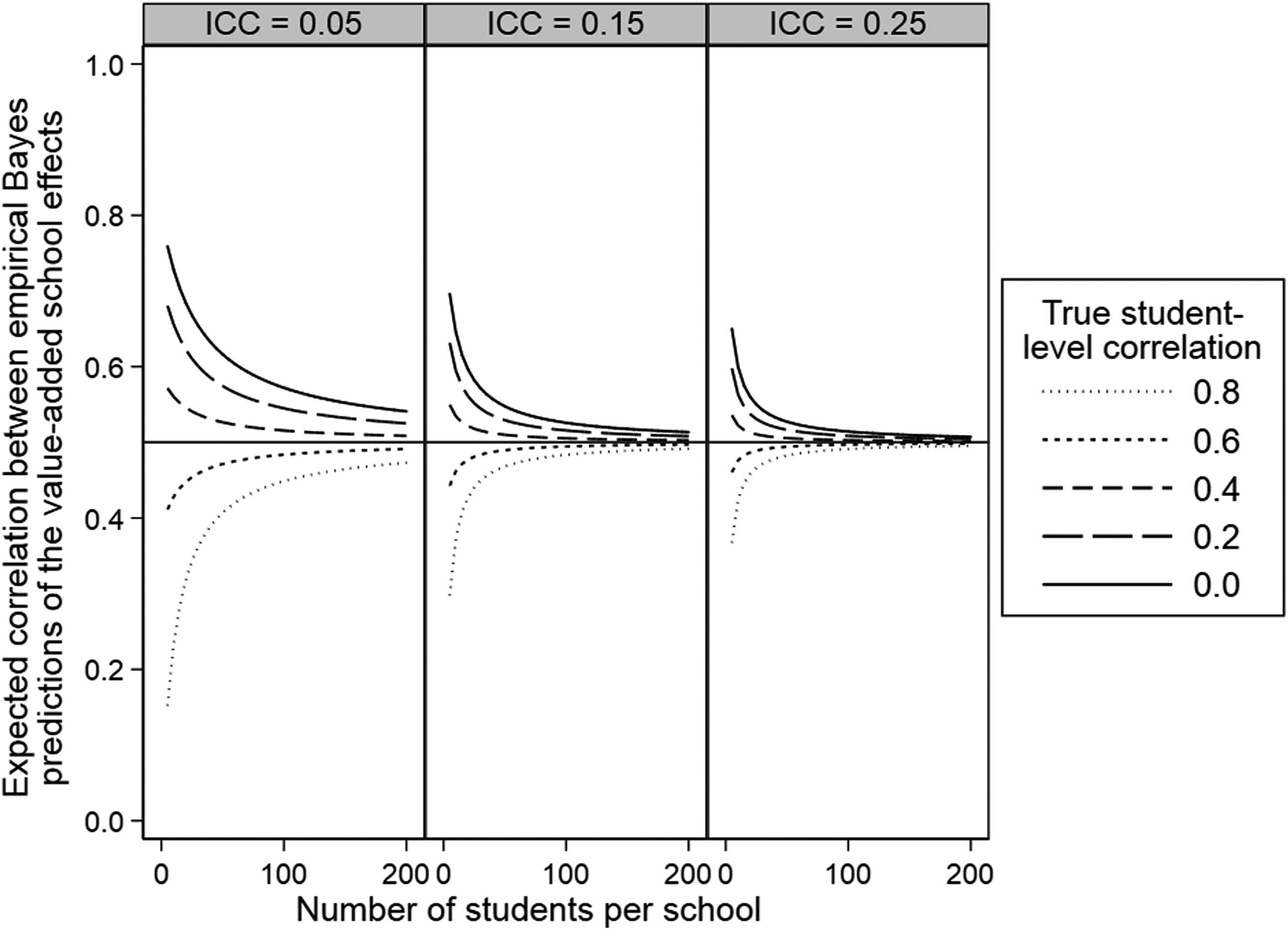
Illustration of the expected correlation between empirical Bayes predictions of the school effects derived from a joint value-added model. The true school correlation is .5. ICC = intraclass correlation coefficient.

Turning our attention to estimating the stability correlation based on empirical Bayes predictions for two different cohorts of students, Equation 7 simplifies somewhat as the student-level correlation is zero by definition. As a result, Figure 2 also simplifies with the only relevant lines now being the most extreme solid lines. Thus, as with correlating empirical Bayes predictions from separately fitted models, correlating empirical Bayes predictions from the jointly fitted model leads to especially biased correlations between school effects calculated for different cohorts, but here the correlation is biased upward whereas for separately fitted models it was biased downward. In contrast to the simplification of Equation 3, the simplification of Equation 7 does not lead to a simple multiplicative correction factor which can be applied to the current biased estimate to recover an unbiased estimate of the stability correlation.

Recall that Thomas et al. (2007) in their study of the stability of school effects using a joint model for 10 cohorts stated that their reported correlations are inflated due to shrinkage and therefore overstate the true stability of school effects. Our results support this statement; the correlations in Figure 2 are biased upward when the true student-level correlation is zero and the magnitude of this bias is largest in settings where there is greater shrinkage, that is, in studies with weaker clustering and smaller school sizes.

Once again, however, it is important to stress that this shrinkage explanation does not imply that simply calculating and correlating unshrunken versions of the empirical Bayes predictions (i.e., maximum likelihood estimates) provides a way to recover unbiased estimates of the true school correlations. Indeed, it can be shown (see Table A1 and online Supplemental Material) that the expression for the correlation between maximum likelihood estimates of the school effects from the joint model is the same as the expression for the correlation based on maximum likelihood estimates of the school effects from separate models. We have already discussed and illustrated the nature of this bias (see Figure 1), and so we do not repeat this here except to note that it follows that the correlation based on the maximum likelihood estimates of the school effects is biased in the opposite direction to that based on the empirical Bayes predictions. In contrast, the expression for the correlation between the reflated empirical Bayes predictions of the school effects is now unbiased (see Table A1 and online Supplemental Material). This makes sense as reflation transforms the empirical Bayes predictions, so that their variances and covariance match the estimated school covariance matrix, and in the joint model, these estimates are unbiased (see Table A1).

When there are multiple subjects or cohorts, the expected correlation between the maximum likelihood estimates of the predicted school effects relating to any two subjects or two cohorts remains the same, as does the correlation between the reflated empirical Bayes predictions. The correlation between the usual empirical Bayes predictions, however, becomes more complex. The covariance matrix between these predictions (Equation 7) expands to accommodate the additional subjects or cohorts, and so the resulting correlation between any pair of subjects or cohorts is a function of all the variance and covariance parameters not just those directly related to the pair of subjects or cohorts under consideration.

4. Illustrative Applications

In this section, we illustrate the separate modeling and joint modeling approaches to estimating the consistency and stability of school effects. In each case, we analyze data on English school students drawn from the National Pupil Database. In our first application, we focus on primary schools and estimating the consistency of school effects on the cohort of students who sat for their age 11 end of primary school national standardized achievement tests in 2014. We analyze their English and math achievement scores and relate these to their student average English and math scores taken 4 years earlier at age 7. In our second application, we shift our focus to secondary schools and estimating the stability of school effects across two consecutive cohorts of students who sat for their age 16 end of secondary school national examinations in 2013 and 2014, respectively. Here, we analyze a single overall achievement score in these examinations and relate these to their student average score in English and math taken 5 years earlier at age 11. We deliberately present two applications relating to two different phases of education to illustrate the important role school size plays in determining the magnitude of the correlation biases. Secondary school cohorts in England are around 5 times bigger than primary school cohorts, and so we expect to see considerably smaller biases in our secondary school stability application than in our primary school consistency application.

In each application, we analyze a random sample of 100 schools and their students from across the country who appear in the UK Government’s own primary school and secondary school value-added models and performance tables. In the primary school consistency application, the data contain 3,400 students in 100 schools. The mean school has 34 students (range: 5–174). Every student has an achievement score in each subject, though this is not a requirement of the analysis. In the secondary school stability application, the data contain 36,400 students in 100 schools: 18,439 students in 2013 and 17,961 students in 2014. The mean school has 182 students per cohort (range: 63–585). Every school appears in both cohorts, but this is also not a requirement of the analysis.

For simplicity, we standardize each achievement score used in each application to have a mean of 0 and a standard deviation of 1. We specify very simple value-added models similar to those used by the UK Government for school accountability and choice purposes (Leckie & Goldstein, 2017). These models regress student achievement at the end of the relevant value-added period on their achievement at the start of the period, gender and free school meal status (a binary measure of student socioeconomic status). Summary statistics for the data analyzed in each application are presented in Tables S1 and S2 in the online Supplemental Material.

We fit conventional random-effects versions of these models as school-level confounding proves not to be an issue in either of our applications (see Section S5 in the online Supplemental Material for an exploration of this issue including a comparison of the parameter estimates from random- and fixed-effects versions of our models). There was therefore no need to fit the more complex Hausman–Taylor random-effects models described in Section 2. We fit all models using MLwiN 3.01 (Rasbash, Charlton, Browne, Healy, & Cameron, 2009) calling the software from within Stata using the runmlwin command (Leckie & Charlton, 2013). We note that these models can be fitted directly in Stata 15 (StataCorp, 2017) using the “mixed” command (Rabe-Hesketh & Skrondal, 2012), but this proved computationally slow for these models.

4.1. Consistency of Primary School Value-Added Effects Across English and Math in 2014

Table 1 presents parameter estimates and standard errors from separate and joint models for primary school students’ age 11 English and math achievement scores in 2014. The separate and joint model parameter estimates are almost identical. However, the joint model estimates two extra parameters, the school or consistency correlation and the student residual correlation. The estimate of the consistency correlation is .786, suggesting that in these data school effects are fairly consistent across English and math. While the covariate adjustments are not our focus, we note that girls make more progress than boys in English but less progress than boys in math; poor students make less progress in both subjects than their more advantaged peers but only significantly so in English.

Table 1.

Parameter Estimates and Standard Errors From Separate and Joint Models for Primary School Students’ Age 11 English and Math Achievement Scores in 2014

Parameter	Separate Models		Joint Model
Parameter	Age 11 English Score	Age 11 Math Score	Age 11 English Score	Age 11 Math Score
β ₀—Intercept	−.002 (.031)	.168 (.033)	−.004 (.031)	.172 (.033)
β ₁—Age 7 score^a	.783 (.011)	.713 (.013)	.783 (.011)	.715 (.012)
β ₂—Female	.092 (.021)	−.296 (.024)	.092 (.021)	−.296 (.024)
β ₃—Free school meal	−.072 (.029)	−.057 (.033)	−.074 (.029)	−.053 (.033)
$σ_{u}^{2}$ —School variance	.072	.075	.071	.075
$σ_{e}^{2}$ —Student variance	.356	.454	.356	.454
ρ_u12–School correlation	—		.786
ρ_e12—Student correlation	—		.369
ICC	.168	.142	.166	.141

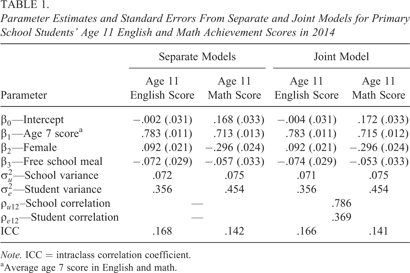
Note. ICC = intraclass correlation coefficient.

^aAverage age 7 score in English and math.

Table 2 presents the variances and correlation between the English and math predicted school effects derived first from the separately fitted models and then from the joint model. The table presents these variances and correlations for maximum likelihood estimates and reflated empirical Bayes predictions of the school effects as well as for the usual empirical Bayes predictions. For ease of comparison, we also include the model-based estimates of these parameters that appeared in Table 1.

Table 2.

Alternative Estimates of the Variances and Consistency Correlation for Different Predicted School Effects Derived From Separate and Joint Models for Primary School Students’ Age 11 English and Math Achievement Scores in 2014

Parameter	Separate Models		Joint Model
Parameter	Age 11 English Score	Age 11 Math Score	Age 11 English score	Age 11 Math Score
$σ_{u}^{2}$ —School variance
Model based	.072	.075	.071	.075
Maximum likelihood	.091	.098	.091	.098
Empirical Bayes	.061	.061	.060	.062
Reflated	.073	.076	.072	.075
ρ_u12—School correlation
Model based	—		.786
Maximum likelihood	.666		.666
Empirical Bayes	.690		.839
Reflated	.690		.786

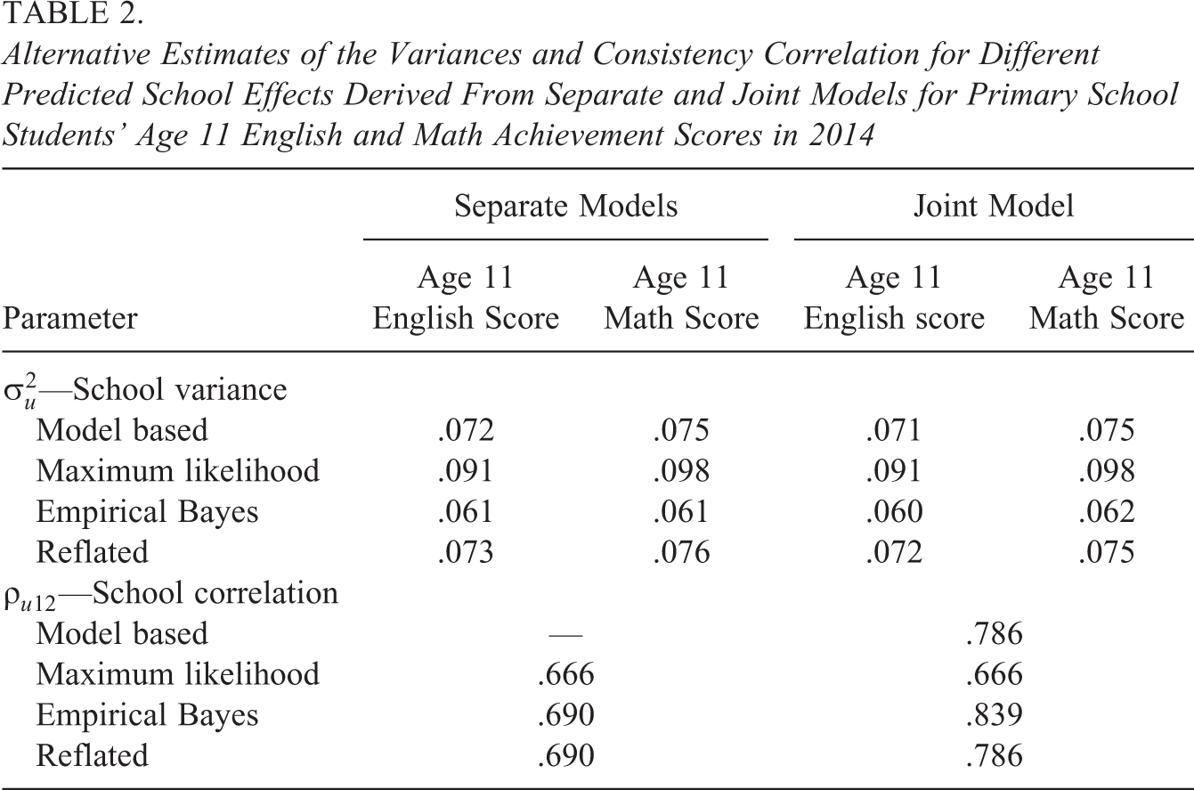
We first consider the correlations between the different predicted school effects derived from the separate models. The correlation between the empirical Bayes predictions of the English and math school effects is .690, substantially lower than the unbiased estimate of .786 derived directly from the joint model. The corresponding correlations based on the maximum likelihood estimates and reflated empirical Bayes predictions are very similar, .666 and .690, with the small difference between all three correlations relating to the unbalanced nature of the data. In terms of the variances, we see that the variances of the maximum likelihood estimates (.091 and .098) are biased upward relative to the unbiased model-based estimates (.072 and .075), while the variances of the empirical Bayes predictions are biased downward (.061 and .061). The variances of the reflated empirical Bayes predictions (.073 and .076) effectively match the unbiased model-based estimates. All of these results and those presented below are consistent with the derivations and discussion presented in Section 3.

Turning our attention to the correlations between the different predicted school effects derived from the joint model. The correlation between the empirical Bayes predictions is .839, substantially higher than the unbiased model-based estimate of .786 as well as the biased correlation of .690 relating to the empirical Bayes predictions derived from the separately fitted models. The correlation between the maximum likelihood estimates of .666 is equal to that based on the maximum likelihood estimates of the school effects derived from the separate models. The correlation between the reflated empirical Bayes predictions is now .786, matching the unbiased estimate exactly. The variances of each set of English and math predicted school effects derived from the joint model are effectively the same as those based on the corresponding predicted school effects derived from the separate models.

4.2. Stability of Secondary School Value-Added Effects in Overall Achievement Across 2013 and 2014

Table 3 presents parameter estimates and standard errors from separate and joint models for secondary school students’ age 16 overall achievement score in the 2013 and 2014 cohorts. As in the primary school consistency application, the separate and joint model parameter estimates are almost identical. Here, the joint model estimates only one extra parameter, the school or stability correlation (the student correlation is implicitly 0, as each student appears in only one cohort). The estimate of this correlation is .747, suggesting that school effects are moderately stable from one cohort to the next.

Table 3.

Parameter Estimates and Standard Errors From Separate and Joint Models for Secondary School Students’ Age 16 Overall Achievement Scores in 2013 and 2014

Parameter	Separate Models		Joint Model
Parameter	Age 16 Score, 2013 Cohort	Age 16 Score, 2014 Cohort	Age 16 Score, 2013 Cohort	Age 16 Score, 2014 Cohort
β ₀—Intercept	−.110 (.029)	−.069 (.028)	−.110 (.029)	−.068 (.028)
β ₁—Age 11 score^a	.620 (.006)	.670 (.005)	.617 (.006)	.670 (.005)
β ₂—Female	.302 (.011)	.224 (.009)	.303 (.011)	.224 (.009)
β ₃—Free school meal	−.184 (.016)	−.214 (.014)	−.180 (.016)	−.217 (.014)
$σ_{u}^{2}$ —School variance	.075	.076	.076	.076
$σ_{e}^{2}$ —Student variance	.455	.351	.455	.351
ρ_u12—School correlation	—		.747
ρ_e12—Student correlation	—		—
ICC	.142	.178	.143	0.179

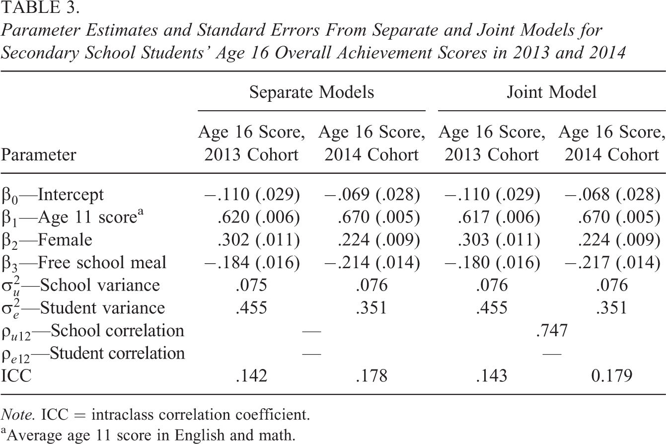
Note. ICC = intraclass correlation coefficient.

^aAverage age 11 score in English and math.

Table 4 presents the variances and correlation between the predicted 2013 and 2014 secondary school effects derived first from the separately fitted models and then from the joint model. The correlation between the empirical Bayes predictions of the 2013 and 2014 school effects derived from the separate models is .719, slightly lower than the unbiased model-based estimate of .747 derived directly from the joint model. Applying the multiplicative correction factor $R_{1}^{- .5} R_{2}^{- .5}$ of 1.029 derived from Equation 6 to 0.719 gives a revised estimate of 0.740, which is much closer to the unbiased model–based estimate. The corresponding correlations based on unshrunken and reflated versions of these predictions are very similar, .722 and .719, respectively.

Table 4.

Alternative Estimates of the Variances and Stability Correlation for Different Predicted School Effects Derived From Separate and Joint Models for Secondary School Students’ Age 16 Overall Achievement Scores in 2013 and 2014

Parameter	Separate Models		Joint Model
Parameter	Age 16 Score, 2013 Cohort	Age 16 Score, 2014 Cohort	Age 16 Score, 2013 Cohort	Age 16 Score, 2014 Cohort
$σ_{u}^{2}$ —School variance
Model-based	.075	.076	.076	.076
Maximum likelihood	.080	.080	.081	.080
Empirical Bayes	.074	.074	.074	.075
Reflated	.076	.077	.077	.077
ρ_u12—School correlation
Model-based estimate	—		.747
Maximum likelihood	.722		.725
Empirical Bayes	.719		.769
Reflated	.719		.747

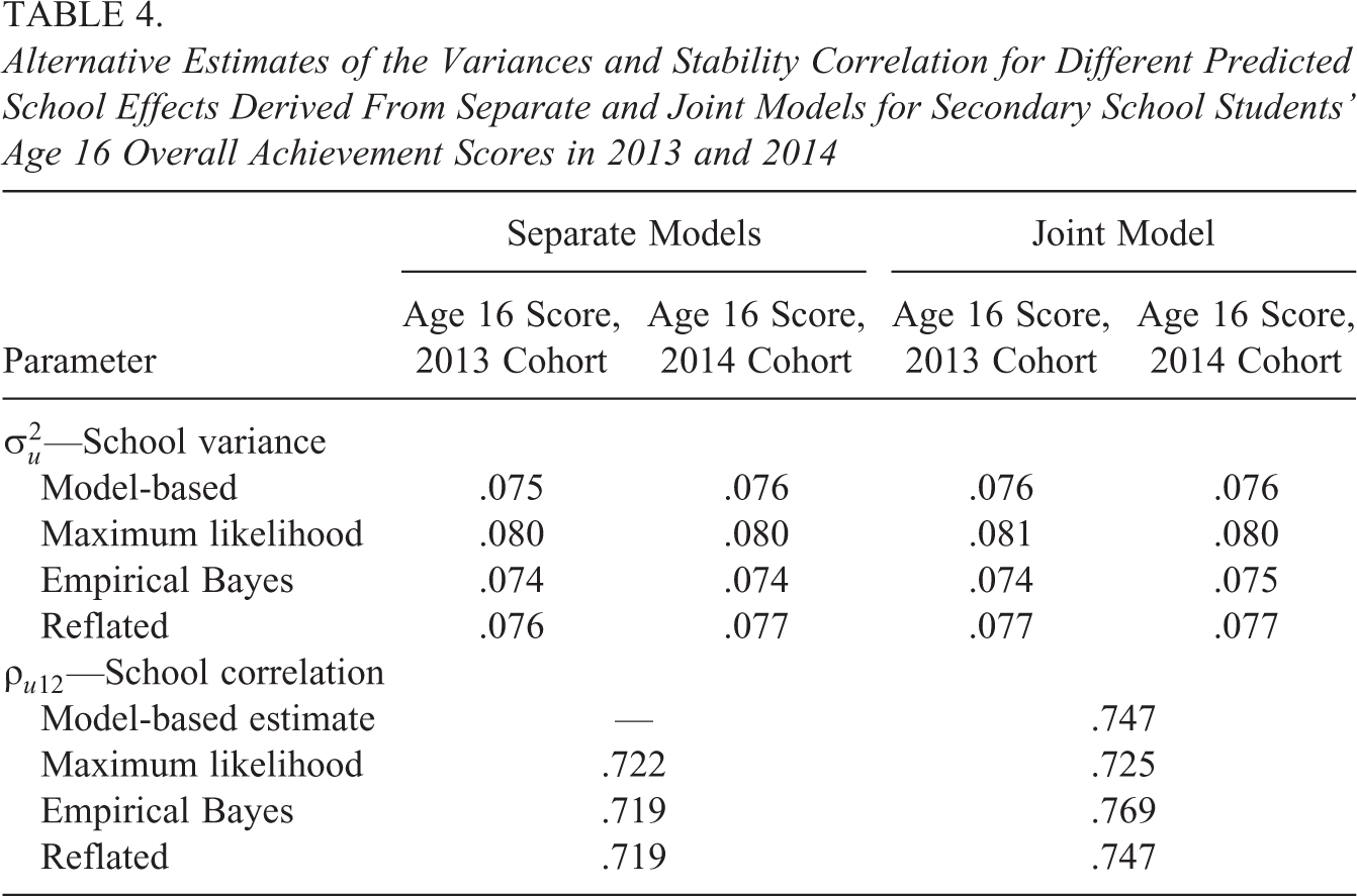
The correlation between the empirical Bayes predictions derived from the joint models is .769, slightly higher than the unbiased model-based estimate of .747. The correlation between the maximum likelihood estimates is .725, effectively the same as that based on the maximum likelihood estimates of the school effects derived from the separate models. In contrast, the correlation between the reflated empirical Bayes predictions is .747 matching the unbiased estimate exactly.

The biases exhibited in this application are far smaller than those exhibited in the primary school consistency application. The principal reason for this are the larger school sizes seen in secondary schools; the mean secondary school cohort has 182 pupils, while the mean primary school cohort has only 34 students. If we retain a random sample of 34 students per school cohort in the current application, refit the separate and joint models and recalculate the stability correlations, the unbiased model-based correlation is now estimated as .756 while the correlation between the empirical Bayes predictions derived from separate models of just .645 is dramatically biased. (As expected, the corresponding correlations between the maximum likelihood and reflated versions of these effects are also .645.) The correlations between the empirical Bayes predictions and maximum likelihood estimates derived from the joint models are also dramatically biased, .832 and .651, respectively.

5. Conclusion

In this article, we have argued that the preferred approach to estimating the consistency and stability of school effects is to fit a joint model to the multiple subjects or cohorts under investigation and to estimate the consistency or stability correlations directly as a function of the model parameters. In contrast, we have shown that the traditional approach of fitting separate models to each subject or cohort and correlating the empirical Bayes predictions of the school effects results in biased correlations. When estimating the consistency of school effects across subjects for a single cohort, the consistency correlations are biased toward the corresponding student-level correlations. Studies employing this approach cannot therefore state whether their consistency correlations are overestimated or underestimated, as they do not estimate this student-level correlation. When estimating the stability of school effects in a single subject across multiple cohorts, the stability correlations are biased toward zero and the expected magnitude of this bias can be calculated without fitting the joint model. We have shown that the bias is a decreasing function of clustering and school size. This does not mean, however, that it is the shrunken nature of the empirical Bayes predictions per se which drives these biases. Indeed, we have shown that simply correlating unshrunken maximum likelihood estimates of the school effects results in the same biased correlations as does correlating reflated versions of the empirical Bayes predictions.

We also explored the consequences of correlating empirical Bayes predictions for multiple subjects or cohorts derived from the joint model since some researchers also follow this approach. We showed that these correlations are also biased. In the case of studying, the consistency or stability correlation between two subjects or cohorts this bias is in the opposite direction to that derived for the correlation between empirical Bayes predictions based on separately fitted models. Thus, in this setting, the consistency of school effects correlation is now biased away from the corresponding student-level correlation, while the stability of school effects correlation is biased away from zero. In common with the separate modeling approach, the bias is again most severe when clustering is low and school size is small. Correlating unshrunken maximum likelihood estimates of the school effects from the joint model also results in biased correlations, but these correlations no longer coincide with the correlations between the empirical Bayes predictions. Indeed, the correlations are the same as those between the maximum likelihood estimates of the school effects derived from separate models and are therefore of the opposite sign to those based on the empirical Bayes predictions based on the joint model. In contrast, the correlations based on reflated versions of the empirical Bayes predictions from the joint model are now unbiased. However, given that unbiased estimates of the consistency and stability correlations are easily obtained directly from the parameters of the joint model, there is no obvious benefit from correlating reflated versions of the empirical Bayes predictions.

In terms of our two illustrative applications, we note that the primary school consistency application showed substantially larger biases than the secondary school stability application and this reflected the smaller size of primary schools. Thus, the biases we have described will clearly be most relevant to studies that have small school sizes either because they study primary schools or because they sample students within schools. The biases we describe are also relevant to studies of the consistency and stability of teacher effects since the number of students per teacher is often very low.

While our focus has been on contrasting different modeling approaches to measuring the consistency and stability of school effects, our study also has implications for school performance monitoring systems that hold schools accountable for their predicted school effects. Here, one could argue that it is the “biased” correlation between the empirical Bayes predictions, which is the correlation of most interest as it is this correlation that would have to be sufficiently high for schools to have faith in the system. However, here too, there is a choice as to whether to fit separate models to multiple subjects or multiple cohorts or a single joint model, as the different modeling approaches produce different empirical Bayes predictions. In particular, the joint modeling approach shrinks the set of effects for each school toward one another as well as toward the overall average, introducing an element of within school smoothing of results that could be argued desirable when predicted school effects are to be used for such high-stakes decisions. For example, in terms of analyzing multiple cohorts, three adjacent cohorts could be jointly modeled and empirical Bayes predictions could be published for the middle cohort. The purpose of the first and last cohorts would then be to smooth the published results of the middle cohort.

We have contrasted the correlations that arise when we correlate the predicted school effects from separate models and also from the joint model versus the directly estimated correlation of the joint model. We have derived our results assuming the joint model is correct, both in terms of the choice of covariates, how they are entered, and in terms of the plausibility of the model assumptions. We have already drawn attention to an important debate raised by Castellano et al. (2014), which questions whether student prior achievement is plausibly independent of the school effects in this setting. In our two applications, however, school-level confounding introduced at most trivial biases to our parameter estimates. Another ongoing debate relates to the extent to which we should additionally adjust for student demographic and socioeconomic characteristics and their school averages in value-added models, with different arguments made depending on the ultimate purpose of these models: school accountability, school choice, or systemwide change (Leckie & Goldstein, 2017; Raudenbush & Willms, 1995). Researchers should also investigate the school effects homoscedasticity and normality assumptions in their data. For example, where there is a subpopulation of schools behaving differently from the rest, there may be a need not only to reflect this in the covariates but to potentially allow different school variances and covariances for these subpopulations (Leckie, French, Charlton, & Browne, 2014; Sani & Grilli, 2010). Even after allowing for such differences, the normality assumption may not be tenable and other distributions may need to be considered. Further work is required to extend our findings to these more complex models.

We note that more elaborate value-added models than the ones described in this article are increasingly applied but here too correlating predicted school effects, whether from separately or jointly fitted models, would be expected to give different correlations to those estimated directly by joint models. For example, while we have focused on analyzing continuous measures of student achievement, some studies will only have access to binary (e.g., pass/fail) or ordinal (e.g., basic/proficient/advanced) measures of student achievement and would have to fit binary and ordinal response versions of the value-added models we have described to study the consistency and stability of school effects. The expressions for the expected correlations based on these models will be more complex than the analytic expressions presented here and will likely have no closed-form but could be explored in future work with simulation studies. In other studies, there is often information on teachers and classrooms as well as schools or on more than two repeated measures of achievement per pupil in each case leading to considerably more complex multilevel models (Ballou, Sanders, & Wright, 2004; Braun & Wainer, 2007; McCaffrey, Lockwood, Koretz, & Hamilton, 2003; McCaffrey, Lockwood, Koretz, Louis, & Hamilton, 2004). Here, too, simulation studies could be used to quantify the expected correlations and biases associated with the different approaches we have discussed.

Finally, it should be realized that while our focus has been on studying the consistency and stability of value-added school effects, the arguments we have made are relevant to applications of multilevel models in general whenever there is interest in interpreting the correlation between random effects. Correlating predicted random effects, whether from separate or joint models, will give biased correlations relative to the directly estimated correlations of the joint model. For example, in some studies, researchers fit separate multilevel models (e.g., students within-teachers models) to different population subgroups (e.g., gender or ethnic groups) and then correlate the predicted random effects across these subgroups to study cluster-level agreement in the adjusted response (e.g., the extent to which male and female students agree on their teacher ratings). These correlations will be biased relative to those obtained from fitting a joint model and estimating them directly. Another example relates to studies where researchers fit separate growth-curve models to repeated measures data (e.g., annual assessment score data) on different outcome measures (e.g., math and reading), only to correlate the growth parameters across outcomes postestimation (i.e., student initial status and growth-rate random effects). Again, this will give biased correlations relative to fitting a joint growth-curve model and estimating the correlations directly. A third example relates to studies where the random effects from a first-step model are used as predictors in a second-step model, for example, when predicting later life outcomes (e.g., high school graduation) from the growth parameters derived from a growth-curve model fitted to earlier life repeated measures data (e.g., annual assessment score data). Here, it is the regression coefficients on the random effects obtained via this separate modeling approach, which will be biased relative to those obtained when fitting the two equations jointly.

Supplemental Material

Supplemental Material - Avoiding Bias When Estimating the Consistency and Stability of Value-Added School Effects

Supplemental Material for Avoiding Bias When Estimating the Consistency and Stability of Value-Added School Effects by George Leckie in Journal of Educational and Behavioral Statistics

Footnotes

Appendix

Table A1 presents expressions for the predicted school effects and their expected or population variances, covariances, and correlations for both the separate and joint modeling approaches and for three different methods for assigning values: maximum likelihood estimation, empirical Bayes prediction, and reflated empirical Bayes prediction. The expressions for the variances, covariances, and correlations assume that the joint model (Equation 3) is the true model and that school size is constant across all schools. See the online Supplemental Material for full derivations and further description.

Acknowledgments

We thank Sophia Rabe-Hesketh and Anders Skrondal for their useful comments and feedback on an earlier draft and the three reviewers and editor for many helpful suggestions on the submitted manuscript.

Declaration of Conflicting Interests

The author(s) declared no potential conflicts of interest with respect to the research, authorship, and/or publication of this article.

Funding

The author(s) disclosed receipt of the following financial support for the research, authorship, and/or publication of this article: This research was funded by UK Economic and Social Research Council grant ES/K000950/1.

ORCID iD

G. Leckie

References

Ballou

Sanders

Wright

(2004). Controlling for student background in value-added assessment of teachers. Journal of Educational and Behavioral Statistics, 29, 37–65.

Braun

H. I.

Wainer

(2007). Value-added assessment. Handbook of Statistics, 27, 867–892.

Carpenter

J. R.

Goldstein

Rasbash

(2003). A novel bootstrap procedure for assessing the relationship between class size and achievement. Journal of the Royal Statistical Society: Series C (Applied Statistics), 52, 431–443.

Castellano

K. E.

Rabe-Hesketh

Skrondal

(2014). Composition, context, and endogeneity in school and teacher comparisons. Journal of Educational and Behavioral Statistics, 39, 333–367.

Doolaard

(2002). Stability and change in results of schooling. British Educational Research Journal, 28, 773–787.

Dumay

Coe

Anumendem

D. N.

(2014). Stability over time of different methods of estimating school performance. School Effectiveness and School Improvement, 25, 64–82.

Goldstein

(1997). Methods in school effectiveness research. School Effectiveness and School Improvement, 8, 369–395.

Goldstein

(2011). Multilevel statistical models (4th ed.). Chichester, England: Wiley.

Goldstein

Rasbash

Yang

Woodhouse

Pan

Nuttall

Thomas

(1993). A multilevel analysis of school examination results. Oxford Review of Education, 19, 425–433.

10.

Gorard

Hordosy

Siddiqui

(2013). How unstable are “school effects” assessed by a value-added technique? International Education Studies, 6, 1–9.

11.

Grilli

Pennoniy

Rampichini

Romeoy

(2016). Exploiting TIMSS and PIRLS combined data: Multivariate multilevel modelling of student achievement. Annals of Applied Statistics, 10, 2405–2426.

12.

Guarino

C. M.

Reckase

M. D.

Wooldridge

J. M.

(2015). Can value-added measures of teacher performance be trusted? Education Finance and Policy, 10, 117–156.

13.

Henderson

C. R.

(1950). Estimation of genetic parameters (abstract). The Annals of Mathematical Statistics, 21, 309–310.

14.

Leckie

Charlton

. (2013). Runmlwin—A program to run the MLwiN multilevel modelling software from within Stata. Journal of Statistical Software, 52, 1–40.

15.

Leckie

French

Charlton

Browne

(2014). Modeling heterogeneous variance-covariance components in two-level models. Journal of Educational and Behavioral Statistics, 39, 307–332.

16.

Leckie

Goldstein

(2009). The limitations of using school league tables to inform school choice. Journal of the Royal Statistical Society: Series A (Statistics in Society), 172, 835–851.

17.

Leckie

Goldstein

(2011). A note on “The limitations of using school league tables to inform school choice.” Journal of the Royal Statistical Society: Series A (Statistics in Society), 174, 833–836.

18.

Leckie

Goldstein

(2017). The evolution of school league tables in England 1992-2016: “Contextual value-added”, “expected progress” and “progress 8.” British Educational Research Journal, 43, 193–212.

19.

Loeb

Candelaria

C. A.

(2012). How stable are value-added estimates across years, subjects and student groups? What we know series: Value-added methods and applications. Knowledge brief 3. Carnegie Foundation for the Advancement of Teaching.

20.

Luyten

(1998). School effectiveness and student achievement, consistent across subjects? Evidence from Dutch elementary and secondary education. Educational Research and Evaluation, 4, 281–306.

21.

(2001). Stability of school academic performance across subject areas. Journal of Educational Measurement, 38, 1–18.

22.

Marks

G. N.

(2015). The size, stability, and consistency of school effects: Evidence from Victoria. School Effectiveness and School Improvement, 26, 397–414.

23.

McCaffrey

D. F.

Lockwood

J. R.

Koretz

D. M.

Hamilton

L. S.

(2003). Evaluating value-added models for teacher accountability (Monograph. PO Box 2138). Santa Monica, CA: RAND Corporation.

24.

McCaffrey

D. F.

Lockwood

J. R.

Koretz

Louis

T. A.

Hamilton

(2004). Models for value-added modeling of teacher effects. Journal of Educational and Behavioral Statistics, 29, 67–101.

25.

Newton

Darling-Hammond

Haertel

Thomas

(2010). Value-added modeling of teacher effectiveness: An exploration of stability across models and contexts. Educational Policy Analysis Archives, 18, 1–27.

26.

Perry

(2016). English value-added measures: Examining the limitations of school performance measurement. British Educational Research Journal, 42, 1056–1080.

27.

Rabe-Hesketh

Skrondal

(2012). Multilevel and longitudinal modeling using Stata (3rd ed., Vol. 1: Continuous responses). College Station, TX: Stata Press.

28.

Rasbash

Charlton

Browne

W. J.

Healy

Cameron

(2009). MLwiN (Version 2.1). Bristol, England: Centre for Multilevel Modelling, University of Bristol. Retrieved from http://www.mlwin.com

29.

Raudenbush

S. W.

Bryk

A. S.

(2002). Hierarchical linear models: Applications and data analysis methods (2nd ed.). Thousand Oaks, CA: Sage.

30.

Raudenbush

S. W.

Willms

J. D.

(1995). The estimation of school effects. Journal of Educational and Behavioral Statistics, 20, 307–335.

31.

Reynolds

Sammons

De Fraine

Van Damme

Townsend

Teddlie

Stringfield

(2014). Educational effectiveness research (EER): A state-of-the-art review. School Effectiveness and School Improvement, 25, 197–230.

32.

Sani

Grilli

(2010). Differential variability of test scores among schools: A multilevel analysis of the fifth-grade Invalsi test using heteroscedastic random effects. Journal of Applied Quantitative Methods, 6, 88–99.

33.

Shavelson

R. J.

Domingue

B. W.

Mariño

J. P.

Molina Mantilla

Morales Forero

Wiley

E. E.

(2016). On the practices and challenges of measuring higher education value added: The case of Colombia. Assessment & Evaluation in Higher Education, 41, 695–720.

34.

Skrondal

Rabe-Hesketh

(2004). Generalized latent variable modeling: Multilevel, longitudinal, and structural equation models. Boca Raton, FL: Chapman & Hall/CRC.

35.

Skrondal

Rabe-Hesketh

(2009). Prediction in multilevel generalized linear models. Journal of the Royal Statistical Society: Series A (Statistics in Society), 172, 659–687.

36.

Snijders

T. A. B.

Bosker

R. J.

(2012). Multilevel analysis: An introduction to basic and advanced multilevel modeling (2nd ed.). London, England: Sage.

37.

StataCorp. (2017). Stata statistical software: Release 15 [Computer software]. College Station, TX: StataCorp LLC. Retrieved from http://www.stata.com

38.

Teddlie

Reynolds

(2000). The international handbook of school effectiveness research. Dayton, OH: Psychology Press.

39.

Thomas

Peng

W. J.

Gray

(2007). Modelling patterns of improvement over time: Value added trends in English secondary school performance across ten cohorts. Oxford Review of Education, 33, 261–295.

40.

Thomas

Sammons

Mortimore

Smees

(1997). Stability and consistency in secondary schools’ effects on students’ GCSE outcomes over three years. School Effectiveness and School Improvement, 8, 169–197.

41.

Townsend

(Ed.). (2007). International handbook of school effectiveness and improvement: Review, reflection and reframing (Vol. 17). Dordrecht, The Netherlands: Springer Science & Business Media.

42.

Wainer

(2004). Introduction to a special issue of the journal of educational and behavioral statistics on value-added assessment. Journal of Educational and Behavioral Statistics, 29, 1–2.

43.

Willms

J. D.

Raudenbush

S. W.

(1989). A longitudinal hierarchical linear model for estimating school effects and their stability. Journal of Educational Measurement, 26, 209–232.

44.

Wilson

Piebalga

(2008). Performance measures, ranking and parental choice: An analysis of the English school league tables. International Public Management Journal, 11, 344–366.

Supplementary Material

Please find the following supplemental material available below.

For Open Access articles published under a Creative Commons License, all supplemental material carries the same license as the article it is associated with.

For non-Open Access articles published, all supplemental material carries a non-exclusive license, and permission requests for re-use of supplemental material or any part of supplemental material shall be sent directly to the copyright owner as specified in the copyright notice associated with the article.

0.00 MB

0.09 MB