
Abstract
Mixture models have been developed to enable detection of within-subject differences in responses and response times to psychometric test items. To enable mixture modeling of both responses and response times, a distributional assumption is needed for the within-state response time distribution. Since violations of the assumed response time distribution may bias the modeling results, choosing an appropriate within-state distribution is important. However, testing this distributional assumption is challenging as the latent within-state response time distribution is by definition different from the observed distribution. Therefore, existing tests on the observed distribution cannot be used. In this article, we propose statistical tests on the within-state response time distribution in a mixture modeling framework for responses and response times. We investigate the viability of the newly proposed tests in a simulation study, and we apply the test to a real data set.
1. Introduction
Recently, research interest has grown in modeling response times next to the item responses in order to investigate individual differences in ability and speed. Focusing on the item response times in addition to the item responses has facilitated various aspects of psychological testing including, for instance, item selection in computerized adaptive testing (van der Linden et al., 1999; Veldkamp, 2016), test design (van der Linden, 2007), and item calibration (T. Wang & Hanson, 2005). In addition, response times have been shown useful in detecting item preknowledge (McLeod et al., 2003), aberrant response patterns (Marianti et al., 2014; van der Linden & Guo, 2008; C. Wang, Xu, Shang, & Kuncel, 2018), and individual differences in the use of solution strategies. For instance, van der Maas and Jansen (2003) showed that response times can give detailed information on the type and duration of different solution strategies children use to solve a balance scale task. Suitable models to enable these inferences concerning individual differences in responses and response times include the model by Roskam (1987) and more recently the hierarchical model by van der Linden (2007, 2009), which was elaborated by Molenaar et al. (2015a).
Besides these applications of response times to individual differences research, response times have been used to facilitate the study of within-subject differences in solution strategies or psychological processes that underlie the responses to psychometric tests and questionnaires. For instance, response times have been used to identify fast guessing (e.g., Schnipke & Scrams, 1997) and within-subject differences in solution strategies (e.g., Molenaar et al., 2016). Other applications include the study of within-subject differences in motivation (Wise & Kong, 2005) and faking on personality test items (Holden & Kroner, 1992).
To facilitate the detection of within-subject differences in responses and response times, various approaches based on mixture modeling have been proposed. For instance, the earliest contribution by Schnipke and Scrams (1997) focused on a two-state within-subject mixture model for the response times only. Here, one state represented rapid-guessing behavior of examinees and the other state modeled the responses of examinees who actually tried to solve the item (i.e., a regular response process). The model by Schnipke and Scrams did not include a latent speed variable but can be seen as one of the first models within this framework. In their model, the mean and variance of the response times are estimated freely for each item in the regular process state, while in the rapid-guessing state, a common mean and variance parameter is assumed to underly the items. On the basis of this model, C. Wang and Xu (2015) and C. Wang, Xu and Shang (2018) proposed a mixture model in which separate measurement models are proposed for modeling the responses and response times in the slower response state, whereas for the faster guessing state, only a guessing parameter is estimated for the responses, and a mean and variance parameter is estimated for the response times. Molenaar et al. (2016) generalized this approach by proposing a mixture model that specifies a measurement model for the responses and a measurement model for the response times separately in each state.
Inspired by the aforementioned models, the hierarchical mixture modeling approach (Molenaar et al., 2016; Schnipke & Scrams, 1997; C. Wang & Xu, 2015; C. Wang, Xu, & Shang, 2018; C. Wang, Xu, Shang, & Kuncel, 2018) that we focus on in this article is a mixture extension of the hierarchical model by van der Linden (2007, 2009) to allow for within-subject differences in ability and speed. In the van der Linden model, between-subject differences in ability level are captured by means of a continuous random latent ability variable
To enable mixture modeling of both the responses and response times, a distributional assumption is needed for the within-state response time distribution. Correct specification of this distribution is important as it has been shown that violations of the assumed response time distribution may bias modeling results for mixture models in general (Vermunt, 2011), for growth mixture models (Bauer & Curran, 2003), and for the hierarchical mixture modeling framework for responses and response times as discussed above (Molenaar et al., 2018). More specifically, Molenaar et al. (2018) showed that if the observed response time distribution differs from the assumed distribution, within-state parameter estimates and information criteria like Akaike’s Information Criterion (AIC; Akaike, 1974), the Bayesian Information Criterion (BIC; Schwarz, 1978), and the consistent AIC (CAIC; Bozdogan, 1987) will be biased, and spurious states will be detected even if there are no states underlying the data. Thus, specifying an appropriate within-state response time distribution is important. In practice, however, it is commonly unknown which type of distribution would fit the within-state response times best. Often, statistically convenient distributions are chosen, for example, the log-normal, the exponential, or the chi-square distribution. These distributions are considered convenient as respectively the logarithmic, the reciprocal, and the square root transformation will result in normally distributed response times. Once a distribution is chosen, this assumed distribution should ideally be tested to ensure that the mixture modeling results are valid. However, testing this distributional assumption is challenging as the within-state distribution is by definition different from the observed distribution since the latter is aggregated over states. That is, if the within-state log-transformed response time distribution is normal, the observed log-response time distribution will be skewed (assuming that the two states differ in their expected log-response time and their log-response time variance). As a result, it is not clear whether skewness in the observed log-transformed distribution reflects a mixture of two states or a misspecification of the response time distribution (Molenaar et al., 2018). Therefore, traditional statistical tests (e.g., the Shapiro–Wilk test [SW test], 1965) on the observed response time distribution cannot be used.
In this article, we propose statistical tests on the within-state response time distribution in the hierarchical mixture modeling framework for responses and response times. Specifically, we propose tests on normality of the transformed response time distribution using the SW test (Shapiro & Wilk, 1965; see also Royston, 1982a, 1982b, 1992) and the Kolmogorov–Smirnov test (KS test; Kolmogorov, 1933; Smirnov, 1948). Although the SW test and the KS test are well-established methods to test a hypothesized distribution to hold for an observed variable, the innovative aspect of the present study is that we apply these tests to investigate a hypothesized distribution to hold for the latent within-state distribution of the hierarchical mixture modeling framework for responses and response times. We focus on the log-transformation for the response times, making our approach a test on log-normality. We prefer to focus on log-normality as this is the most commonly used assumption in mixture modeling of response times. However, the proposed methodology can readily be used to test for other distributions by using a different response time transformation. That is, one can consider for instance the square root transformation to test for a chi-square distribution and the reciprocal transformation to test for an exponential distribution. In addition, for the KS test, it is straightforward to accommodate any other distribution (e.g., the Weibull, ex-Gaussian, or Wald distribution) as long as its cumulative distribution function exists and can be evaluated.
The proposed normality tests can be used for various types of (response time) mixture models; however, in this study, we apply the tests to the Markov-dependent item states model and the independent item states model (Molenaar et al., 2016). This article is organized as follows: First, we discuss the hierarchical mixture modeling approach with log-response times. Next, we present the normality tests for the within-state response time distribution. We then present a simulation study to investigate the performance of the different normality tests. In addition, we illustrate the use of the tests by means of a real data application, and we end with a general discussion.
2. The Hierarchical Mixture Modeling Approach
In the hierarchical mixture modeling approach (Molenaar et al., 2016; Schnipke & Scrams, 1997; C. Wang & Xu, 2015; C. Wang, Xu, & Shang, 2018), an item-specific latent class variable
Although the latent class variable
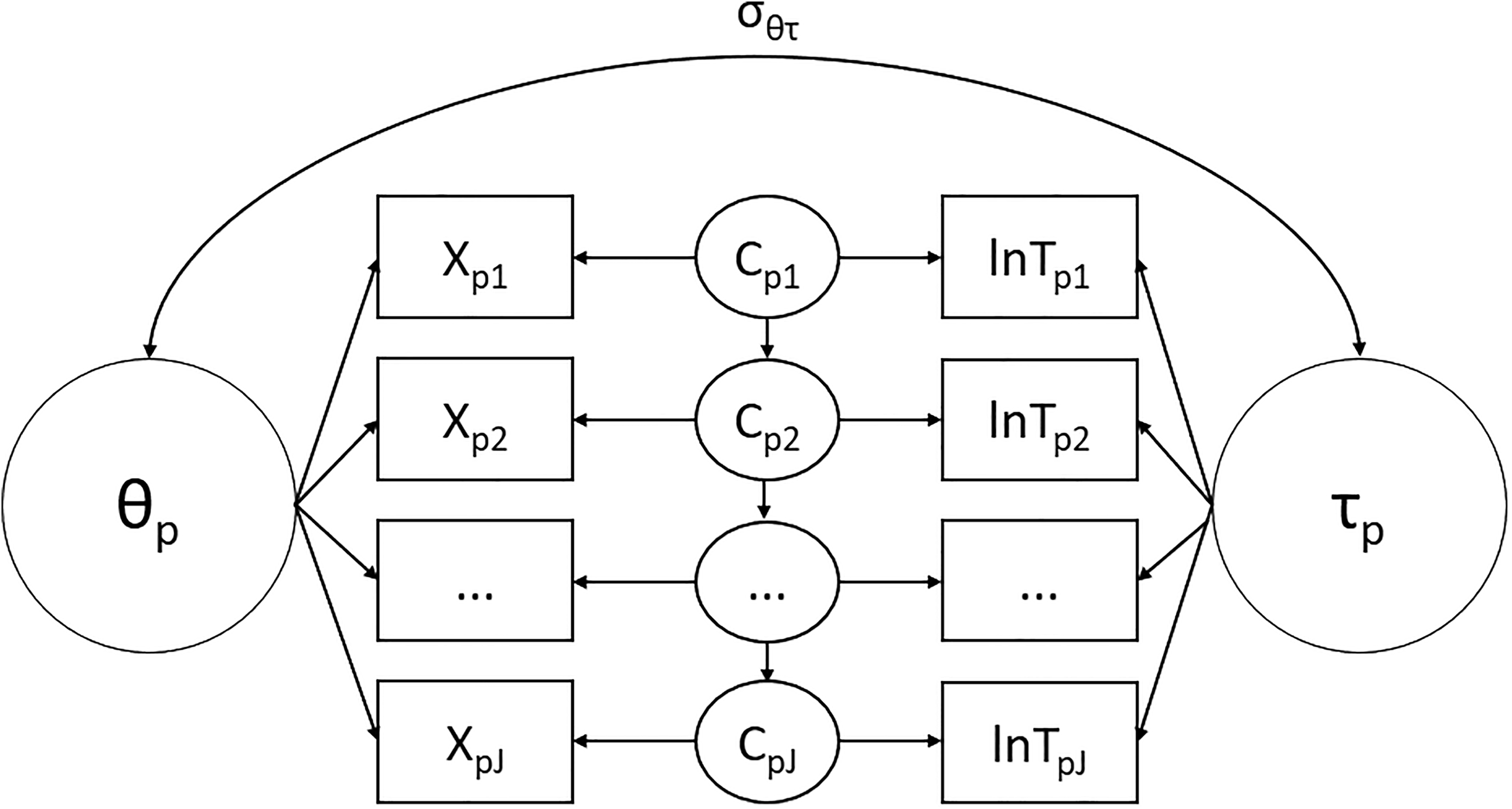
In order to separate the effects of the item, the person and the latent class variable

where
Although other models have been proposed as well, a normal one-factor model is commonly assumed for modeling the log-response times (van der Linden, 2007). Here, we thus assume the log-response times to follow a conditional multivariate normal distribution. As follows,
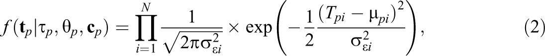
with

where
Next, by assuming a bivariate normal distribution for the latent ability variable
where
In the hierarchical mixture modeling framework, the item-specific latent class variables are commonly assumed to be independent from item to item. However, in practice, these latent class variables may be dependent, for instance, if a respondent guesses on one item, they may be more likely to guess on the next item. To account for such a possible dependency between the latent class variables in the hierarchical mixture framework, Molenaar et al. (2016) also considered a model with a time homogenous first-order Markov-structure on the item-specific latent class variables. As a result, in this model,

where
Markov-dependent item states model.
3. Normality Tests
In the model discussed above, the log-response times within each state are assumed to follow a normal distribution. To test this assumption, we use the SW test and the KS test. Specifically, we propose the following procedure: First, the hierarchical mixture model is fit to the responses and response times. Next, the resulting posterior state probabilities are obtained for each response which in turn are used to draw posterior state assignments to state 0 or 1 for each person’s response to each item. Then the normality tests are conducted on either (1) the response times in state 0 and state 1 according to the posterior state assignment or (2) on the response times weighted by the posterior state probabilities.
The rationale for the above procedure is that if the within-state log-response time distribution is correctly specified, the resulting posterior state probabilities and posterior state assignments are correct. As a result, the SW and KS test statistics will follow their theoretical distribution under the null hypothesis of normality. However, if the within-state log-response time distribution is incorrectly specified, the resulting posterior state probabilities and posterior state assignments are wrong, and the SW and KS test statistics will not follow their null distributions. Below we discuss the SW and KS tests and apply them to the mixture modeling framework.
3.1. SW Test
The SW test, also called the W test for normality, tests the null hypothesis that an observed variable comes from a normally distributed population. Since the original test as proposed by Shapiro and Wilk (1965) could not be used for sample sizes larger than 50, Royston (1982b, 1992) extended it to sample sizes up to 2,000. Then, suppose that
where

where
3.2. KS Test
The KS test is a nonparametric goodness of fit test, which measures the distance between an empirical distribution function of a sample and a hypothesized cumulative distribution function (the one-sample KS test) or which compares the distribution functions of two samples (the two-sample KS test). Here, we will focus on the one-sample KS test for testing the within-state response time distribution of item i for normality, which is defined by

where

where Xp denotes the response time of respondent p on item i, with
Since the posterior state probabilities differ for each respondent on each item they are taken into account by including them as weights in the KS test, Equation 9 needs to be modified to account for the weighted response times (Monahan, 2011). The empirical distribution function can be estimated by

where
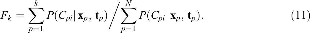
As follows,

Like in the unweighted case, the p value of
4. Simulation Study
4.1. Method
In the simulation study, we compared the performance of the unweighted SW test, the unweighted KS test, and the weighted KS test. Data are simulated according to nine different scenarios, mostly based on Molenaar et al. (2018) who found biased modeling results of the hierarchical mixture model in the case of nonnormality. The first three scenarios concern Markov mixture models that include Markov-dependent item states, the next three scenarios concern mixture models with independent item states, and the final three scenarios are generated according to a baseline model that does not include item states (i.e., a static model without mixtures). The scenarios differ in the distribution that is used for the log-response times, which is a normal, a truncated, or a skewed distribution. The responses are modeled using the two-parameter logistic model, with item parameters
The three Markov mixture model scenarios are the following: Normal Markov mixture: In this scenario, we use the Markov-dependent item states model with normal log-response times to simulate the data. We use Truncated Markov mixture: In this scenario, the data are generated using the same parameter values as in the normal Markov mixture scenario above. However, now we use a right-truncated normal distribution for the log-response times, with truncation at Skewed mixture: Here, the data are generated using the same parameter values as in the normal Markov mixture scenario. However, the normally distributed log-response times are transformed using a Box–Cox transformation (Box & Cox, 1964). In general, the transformation is used to transform skewed variables in such a way that they are closer to a normal distribution. Here, we use the transformation the other way around, so that we transform the normally distributed log-response times into skewed variables using the Box–Cox transformation. That is, we transform the normally distributed log-response times using
Figure 2 shows the resulting log-response time distribution of an arbitrary item from an example run of the three different Markov mixture model scenarios. Note that in the truncated scenario, the log-response times are negatively skewed, while in the skewed scenario, the log-response times are positively skewed.
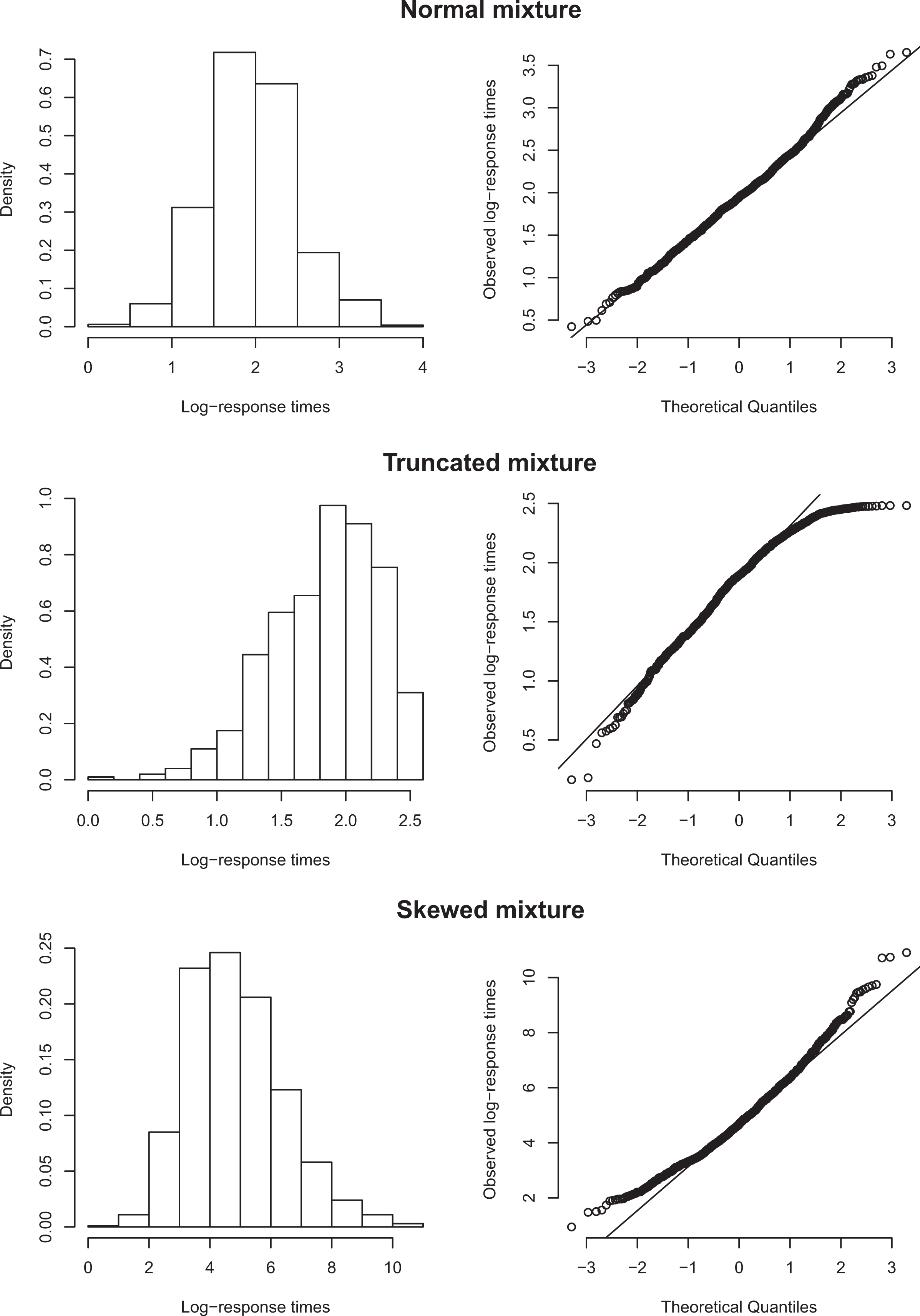
Example run for a random item for normal, truncated, and skewed mixture model scenarios.
In the three independent mixture scenarios, we used the same parameter values and setup as for the Markov mixture scenarios above; however, the item states are assumed to be independent, that is, the Markov structure is omitted (i.e., Normal baseline: In this scenario, the log-response times are normally distributed. The item parameters are as follows: The discrimination parameters for all items are set to Truncated baseline: Here, the data are generated using the same parameter values as in the normal baseline scenario. Like in the truncated mixture model scenario, we use a right-truncated normal distribution for the log-response times, with truncation at Skewed baseline: Here, the data are generated using the same parameter values as in the normal baseline scenario. However, like the skewed mixture model scenario, the normally distributed log-response times are transformed using a reverse Box–Cox transformation (Box & Cox, 1964), with the same value for
5. Results
For the truncated scenarios, convergence problems occurred in
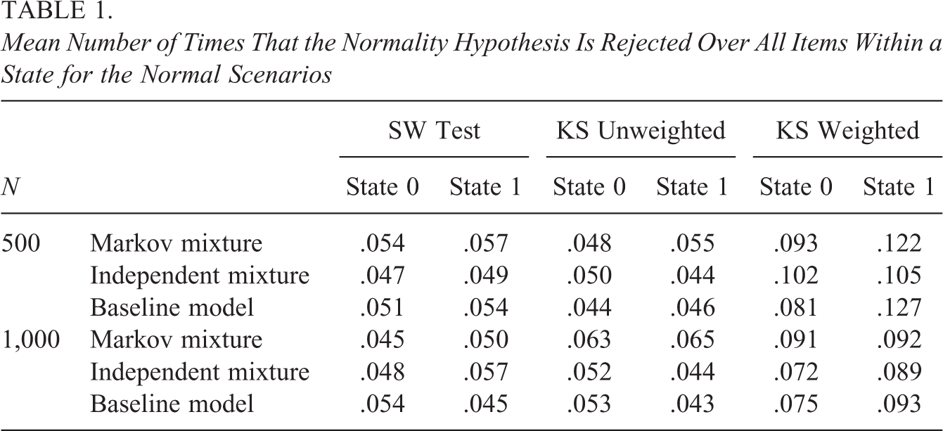
Mean Number of Times That the Normality Hypothesis Is Rejected Over All Items Within a State for the Normal Scenarios
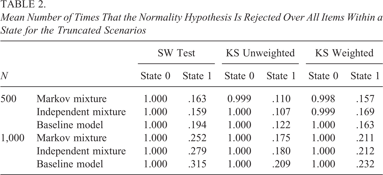
Mean Number of Times That the Normality Hypothesis Is Rejected Over All Items Within a State for the Truncated Scenarios
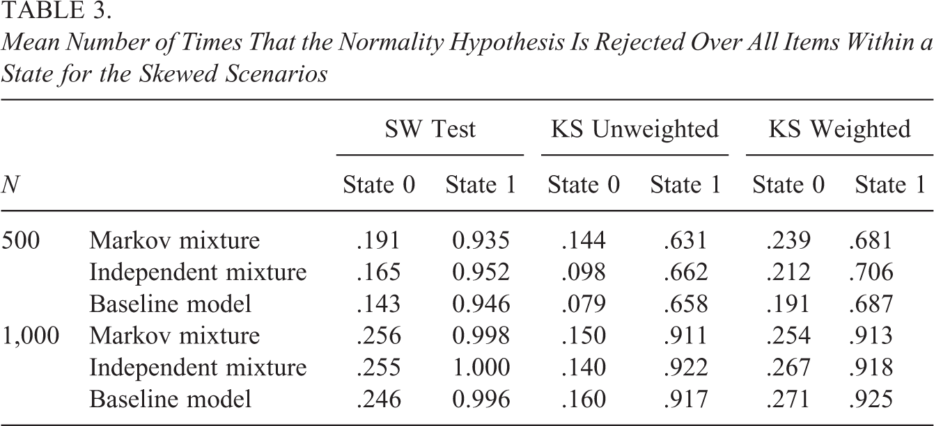
Mean Number of Times That the Normality Hypothesis Is Rejected Over All Items Within a State for the Skewed Scenarios
First, for the normal scenarios in Table 1, these proportions indicate the Type I error rate of our approach. Ideally, these rates are close to the level of significance for the tests to be viable. As can be seen from the table, for the Markov mixture, the independent mixture, and the baseline scenarios, the results are similar. That is, the SW test, and the unweighted KS test have acceptable Type I error rates. In addition, the weighted KS test is associated with an inflated Type I error rate.
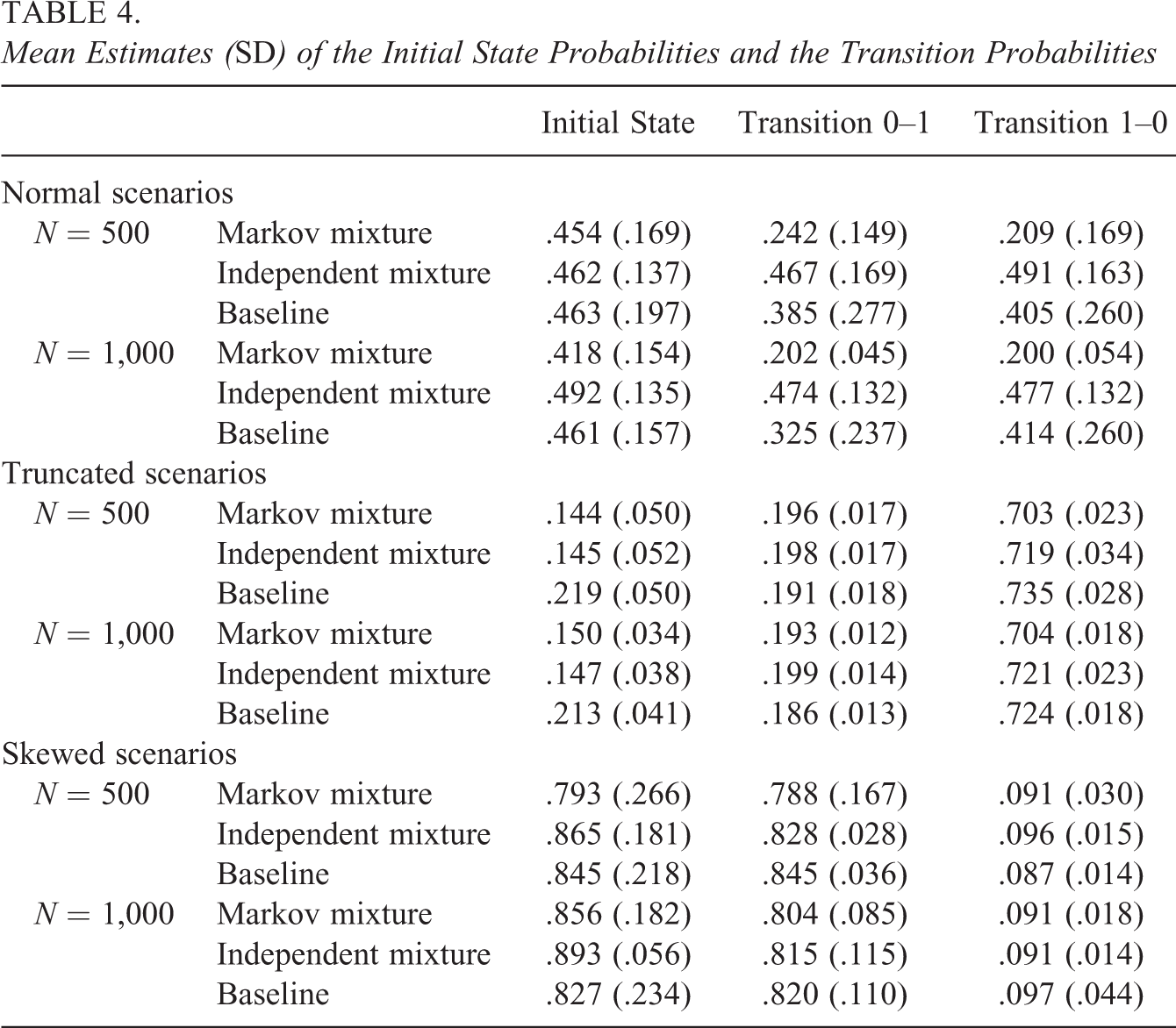
For the truncated and skewed scenarios, the mean proportion of normality rejections reflects the power to detect within-state departures from normality. Here, we used Cohen’s (1988, p. 56) rule of thumb, considering a power coefficient of .80 or higher to be acceptable. As can be seen from Tables 2 and 3, the results indicate that generally the power is acceptable in one state and substantially smaller in the other state. In the truncated scenario, State 0 is associated with larger power, while in the skewed scenario, State 1 is associated with larger power as compared to State 0. This can be explained from Table 4 which contains the average initial state parameter estimates for State 1, together with the transition parameters in the different scenarios (i.e., the table reflects the proportions of persons in the different states). As can be seen from the mean initial state parameter estimates for State 1, in the truncated scenario, State 0 (slower state; larger log-response times) is the larger state, and in the skewed scenario, State 1 (faster state; smaller log-response times) is the larger state. This is due to the log-response times being positively skewed in the skewed scenario and negatively skewed in the truncated scenario (as mentioned above). As a result, due to these larger sample sizes in State 0 for the truncated scenarios and State 1 for the skewed scenarios, power differs between the two states. That is, when fitting a normal mixture to nonnormal data, the nonnormality is best detected in the largest state. Furthermore, even though class sizes are comparable, power tends to be larger in the larger state of the truncated scenarios when compared to the larger state of the skewed scenarios. This is due to the fact that the truncated distribution departs more from normality than the skewed distribution (see Figure 2). In general, the power of the KS tests (weighted and unweighted) is smaller as compared to the SW test. We return to this point in the discussion. Furthermore, the weighted KS test has slightly more power as compared to the unweighted KS test (but is also associated with an increased Type I error rate, see above).
Mean Estimates (SD) of the Initial State Probabilities and the Transition Probabilities
5.1. Conclusion
Taken together the above, Type I error rate and the power of the proposed tests seem acceptable for the SW test and the unweighted KS test with more power for the SW test. The weighted KS test is associated with an inflated Type I error rate. There are no important differences between the Markov mixtures, independent mixtures, and baseline model. It turns out that, generally, violations of normality are only detected in one of the states. We note that of course the power of our approach depends on the severity of the normality violations (this is why the power seems somewhat larger in the truncated scenario as compared to the skewed scenario: the data in the truncated scenario is heavier skewed). In that sense, we consider our simulation study as a prove of principle (i.e., given the effect size we have chosen, we demonstrated that the approach is viable).
Our results indicate that nonnormality is detected if the data contain nonnormal mixtures (i.e., the Markov mixture and independent mixture scenarios) or if the data are nonnormal without mixtures (i.e., the baseline scenarios). In practice, where one does not know the data generating model, a significant normality test thus indicates that (1) the data follow a mixture model with a nonnormal within-state distribution or (2) the data are nonnormal but do not contain mixtures. For the present purposes, the distinction between (1) and (2) is not of importance as the implications are the same: In both cases, there is no mixture of normal distributions in the data, so the results of a normal (Markov-)mixture model should not be trusted. If our proposed tests are insignificant in both states, it can safely be concluded that (1) the data follow a mixture model with a normal within-state distribution or (2) the data are normal without mixtures (i.e., the baseline scenario’s). As in both cases, the (within-state) data are normal, (1) and (2) can be distinguished by comparing the baseline model and the mixture models using common information criteria (e.g., BIC and CAIC) as demonstrated by Molenaar et al. (2018). Therefore, we propose the procedure summarized in the flow chart in Figure 3. That is, first, the fit of a normal (Markov-)mixture model is compared to that of a normal baseline model. If the baseline model fits better, it can be concluded that the transformed response times are normally distributed and that there is no mixture of normal distributions underlying the data. If the mixture model fits better, one can consult the statistics proposed in this article. If these statistics are insignificant in both states, it can be concluded that there is a true mixture of normal distributions underlying the response time data, and the results of the mixture model can be validly interpreted. However, if the proposed statistics are significant, it can be concluded that there is no mixture of normal distributions underlying the data, and the results of the normal (Markov-)mixture model cannot be trusted.
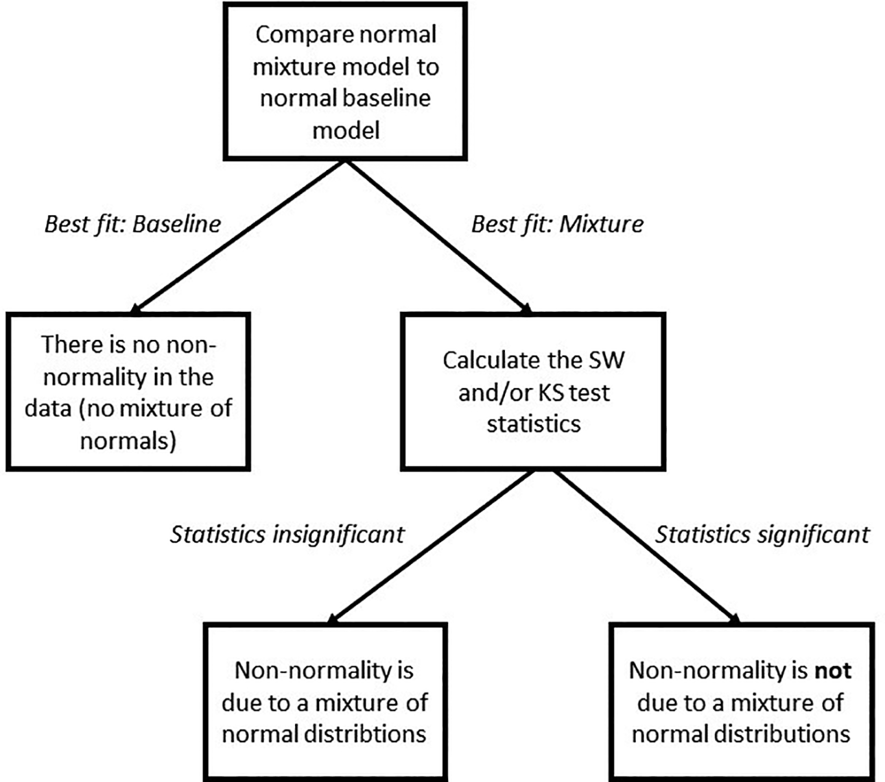
A flowchart of the proposed procedure using the Shapiro–Wilk or Kolmogorov–Smirnov statistics.
6. Application
The within-state normality tests are illustrated by means of a real-data application. The data consist of the responses and response times of 389 psychology freshman of the University of Amsterdam to 28 items of the knowledge subtest of the Dutch version of the Intelligence Structure Test (Amthauer et al., 2001). The knowledge subtest measures essential types of knowledge, which people acquire in schools, higher education and other educational institutions, as well as daily life knowledge acquired from within their culture (Hogrefe Ltd., 2016). The items in the subtest cover a broad range of topics, like economics, geography, mathematics, history, art and culture, natural sciences, and daily life facts (de Vries, 2017). The items are dichotomously scored, with 0 indicating a false response and 1 indicating a correct response. Looking more closely at the response time distributions, Figures 4 and 5 show for a selection of items that they are not normally distributed. The observed response time distributions seem skewed, and the question is whether this nonnormality can be explained by a mixture of a fast and a slow state or whether there is an alternative explanation.
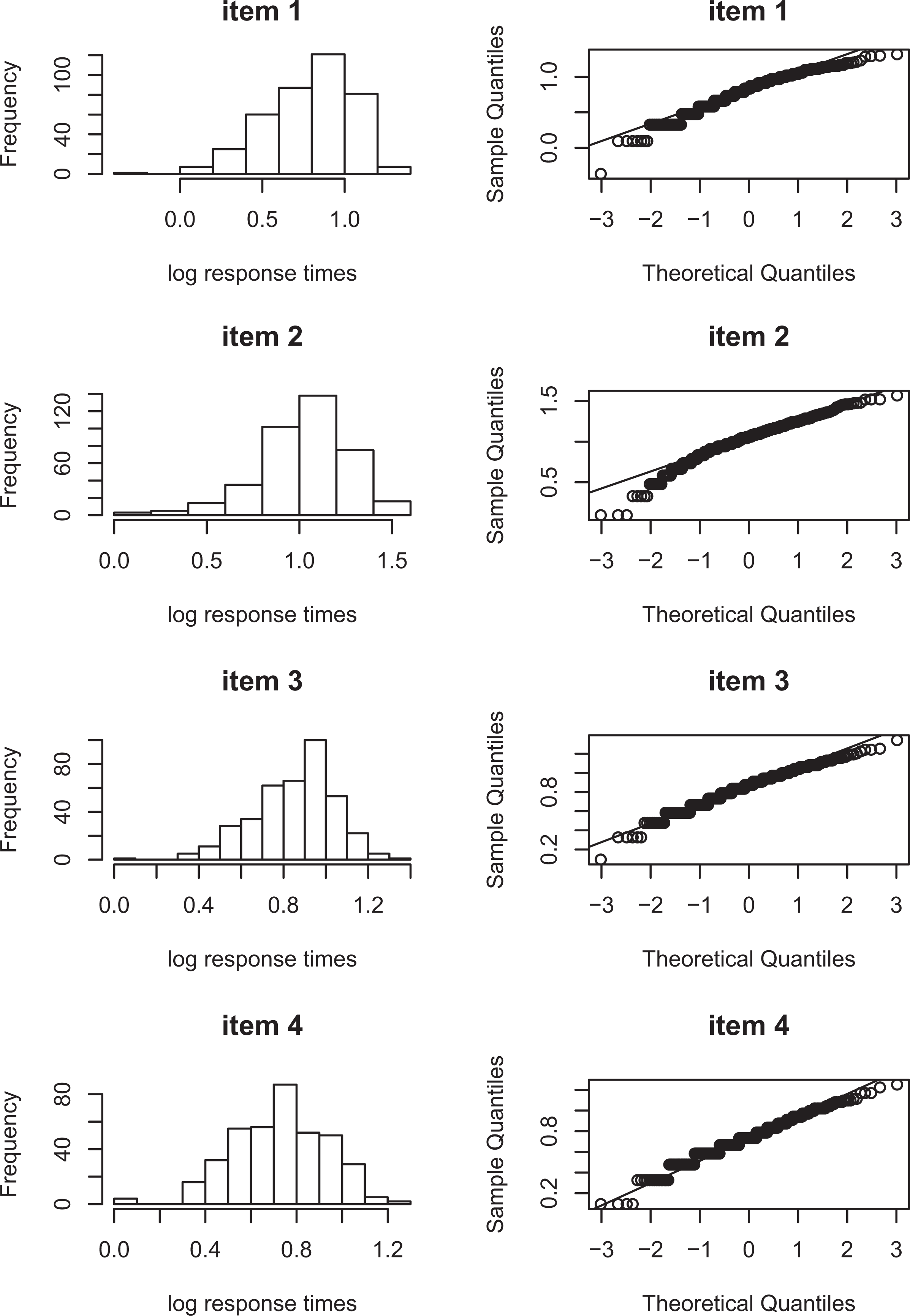
Item score distributions for items 1–4.
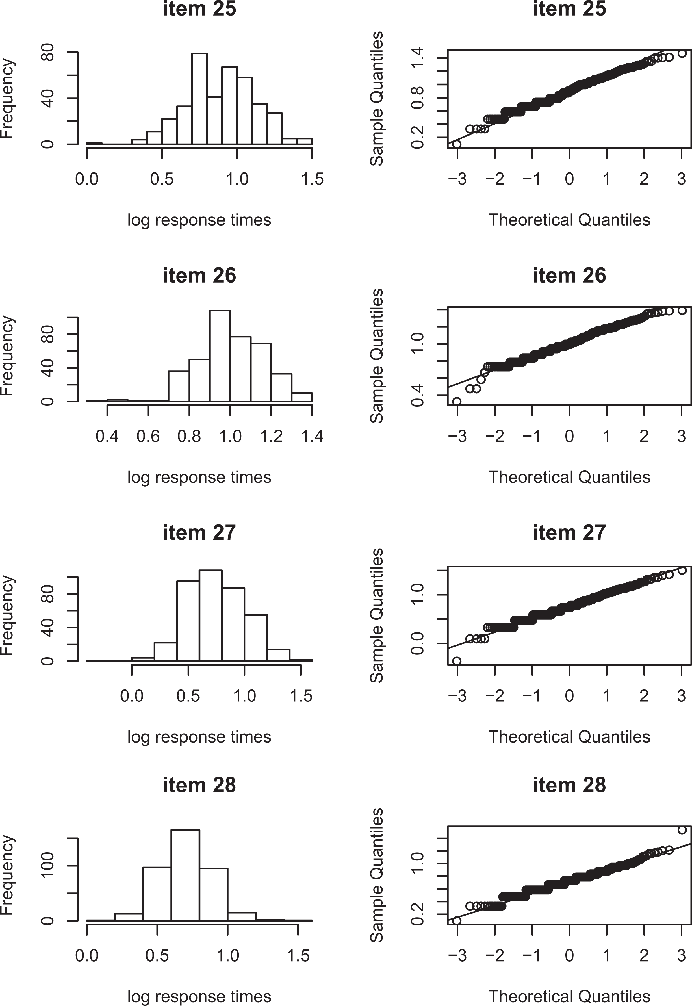
Item score distributions for items 25–28.
In the paper by Molenaar et al. (2016) mixture models with various types of Markov dependencies are fitted to the data and are shown to fit better than a baseline model without item states. However, as the modeling results of a fitting mixture model with a Markov dependency are only interpretable if the assumed normal distribution for the log-response times holds, we test this assumption using the proposed methodology.
Using a significance level of
Number of Nonnormal Items Within Each State
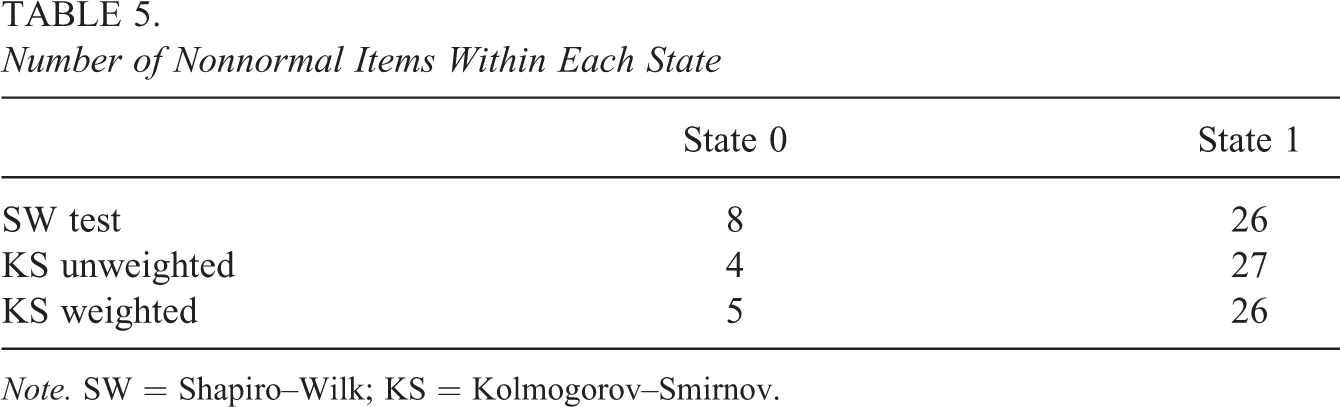
Note. SW = Shapiro–Wilk; KS = Kolmogorov–Smirnov.
7. Discussion
If the within-state response time distribution in the hierarchical mixture modeling framework is misspecified, parameter estimates and model fit indices will be biased and spurious states can be detected in the data as a result. Therefore, in this article, we proposed statistical tests for normality of the within-state log-response time distribution.
In a simulation study, we found that violations of nonnormality can successfully be detected using our tests based on the SW and KS tests. Most importantly, our test has demonstrated an acceptable Type I error rate, which indicates that our test can be used to successfully identify situations where normality holds, and where model fit indices like BIC and CAIC can successfully be used to test between models that include and do not include normal mixtures. If normality is violated, it cannot be concluded whether the violations of normality are due to within-state nonnormality or due to observed nonnormality. However, in such cases, normal mixture modeling should not be adopted anyway, and our test is shown to be a good indicator for such situations.
We also found that the weighted and unweighted KS tests had a slightly increased Type I error rate. In addition, the SW test was associated with larger power as compared to the KS tests. This is line with for instance Razali and Wah (2011), Stephens (1974), and Yap and Sim (2011) who all noted that the KS test in general tends to have smaller power than the SW test. In addition, Shapiro et al. (1968) furthermore showed that in the case of misspecifying the parameters of the hypothesized null distribution, the power and Type I error can be influenced. Type I error rates at the 5% significance level can increase to 61% for a sample size of 50, and the effect becomes more pronounced when sample size increases. Monahan (2011) on the other hand noted that since the KS tests are less powerful, it should not be used in small samples but could be used in larger samples. Although the SW test thus seems preferable over the KS test in the present study, the KS test is more flexible as it can be used to test any assumed distribution, where the SW test can only be used on distributions that can be transformed to a normal one.
As noted above, if in practice, normality is rejected, it is advisable to not interpret the modeling results since they are unreliable. An alternative in that case may be to categorize the response times and use a model for categorical variables as is shown in the application. As Molenaar et al. (2018) showed, such an approach hardly produces parameter bias and false positives with respect to states underlying the data. Furthermore, the approach is comparable to the parametric within-subject mixture modeling approach regarding power. A second solution would be to use a nonparametric or semi-parameter alternative for modeling the responses and response times. However, such an approach is yet to be developed. The semi-parametric models by C. Wang, Fan, et al. (2013) and C. Wang, Chang, and Douglas (2013) can possibly provide a point of departure.
In this article, we have assumed a Markov structure for the dependency between the states. However, the present approach to test for normality is equally amenable to mixture models without Markov structure (e.g., the model by C. Wang & Xu, 2015). In the simulation study, we did not find any important differences between the scenario’s in which the data included a Markov structure and scenario’s in which the data did not included a Markov structure. However, if the Markov dependency becomes stronger (i.e., higher transition probabilities), power for a Markov model may be larger.
Another aspect of the present approach is that of the fit of the mixture model under consideration. That is, we tested for normality by assuming a certain mixture model (in this case, a Markov-dependent item states model). We showed that minor departures from normality can be detected if the model is otherwise correctly specified. If the initial mixture model is misspecified, false positives may arise. The severity of this inflation will depend on the size of the misfit. We therefore think that, first, in practice, were—hopefully—a researcher has a well (theoretically) motivated model that is not severely misspecified, the consequences will not be large. Second, the consequences of this inflation do not have serious consequences as also discussed with respect to the baseline model above. That is, if the tests proposed in the present article are significant, the conclusion should be that the results of the mixture model cannot be trusted.
The normality tests presented in this article are all tests for univariate normality. Testing normality thus needs to be conducted on an item-by-item basis, so in practice, a correction for multiple testing is appropriate (e.g., a Bonferroni or Bonferroni–Holm correction). A focus of future research may be the development of an overall test for multivariate normality, which considers all items at once. Then, the present univariate tests can be used as post hoc tests to investigate whether individual items are responsible for violations of the assumed distribution.
Footnotes
Appendix
Even though
where
for
After calculation of the approximated
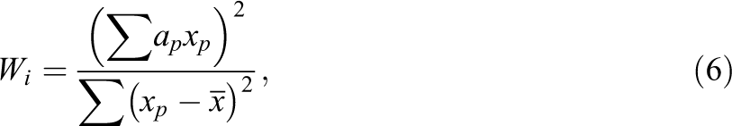
For
As follows, the p value of Wi can be found by using
Declaration of Conflicting Interests
The author(s) declared no potential conflicts of interest with respect to the research, authorship, and/or publication of this article.
Funding
The author(s) disclosed receipt of the following financial support for the research, authorship, and/or publication of this article: The research was supported by a grant from the Dutch Research Council (NWO): VENI-451-15-008.