
Abstract
Disengaged item responses pose a threat to the validity of the results provided by large-scale assessments. Several procedures for identifying disengaged responses on the basis of observed response times have been suggested, and item response theory (IRT) models for response engagement have been proposed. We outline that response time-based procedures for classifying response engagement and IRT models for response engagement are based on common ideas, and we propose the distinction between independent and dependent latent class IRT models. In all IRT models considered, response engagement is represented by an item-level latent class variable, but the models assume that response times either reflect or predict engagement. We summarize existing IRT models that belong to each group and extend them to increase their flexibility. Furthermore, we propose a flexible multilevel mixture IRT framework in which all IRT models can be estimated by means of marginal maximum likelihood. The framework is based on the widespread Mplus software, thereby making the procedure accessible to a broad audience. The procedures are illustrated on the basis of publicly available large-scale data. Our results show that the different IRT models for response engagement provided slightly different adjustments of item parameters of individuals’ proficiency estimates relative to a conventional IRT model.
Introduction
Large-scale assessments of achievement attempt to assess what individuals know and can do.
In order to provide unbiased results, individuals should ideally answer all items with full engagement (Wise & Smith, 2016). However, this requirement is often not fulfilled, especially in low-stakes assessments that have no consequences for individuals (List et al., 2017). Disengagement is considered a threat to the validity of results, because it may lead to lowered proficiency estimates (Wise, 2015) and biased item parameter estimates (Schnipke & Scrams, 1997).
Since the advent of computerized testing, item response times are most often used to identify disengaged responses. In recent years, a number of item response theory (IRT) models for response engagement that augment item responses by response times have been proposed (Pokropek, 2016; Ulitzsch et al., 2020; Wang & Xu, 2015; Wang et al., 2018). These models have the desirable properties of not requiring explicit classifications of engaged and disengaged responses, of reducing bias in item parameter estimates without discarding responses, and of providing estimates of proficiencies that are adjusted for disengagement. The IRT models build on different assumptions and might therefore give different results. However, in real applications, decisions for one specific model are complicated by the fact that many models have not been implemented in widely accessible statistical software. This limits the applicability of IRT models in practice, although many large-scale programs have made item-level data including response times available (e.g., Goldhammer et al., 2016; OECD, 2017).
The aims of the present article are: (1) to summarize the assumptions underlying the classification of response engagement, (2) to outline how these assumptions are embedded in existing IRT models for response engagement, (3) to present some extensions of these models, and (4) to introduce a flexible multilevel mixture IRT (MM-IRT) framework in which IRT models for response engagement can be specified and estimated.
The MM-IRT framework builds upon the widespread Mplus program (Muthén & Muthén, 1998), thereby making IRT models for response engagement accessible to applied researchers. All models can be estimated by marginal maximum likelihood (MML) with the expectation maximization algorithm (EM; Darrell Bock & Lieberman, 1970), including those models that have previously been estimated only in a Bayesian framework (e.g., Ulitzsch et al., 2020; Wang et al., 2018). Although Bayesian estimation has many advantages, it comes at the price of long estimation times. This renders Bayesian estimation impractical in the case of large sample sizes, which are typical for large-scale assessments. In contrast, MML estimation is mainly limited by the number of dimensions that need to be numerically integrated, and it can be applied in fairly large samples.
The remainder of this article is structured as follows. In the next section, we outline the rationales underlying traditional procedures for classifying response engagement. We then describe the IRT models for response engagement that have been suggested in the literature, discuss their assumptions, and provide some extensions that make the models more flexible. Following that, we introduce the MM-IRT framework and show how the models presented are specified in this framework. The framework is illustrated with publicly available data taken from the program for the international assessment of adult competencies (http://www.oecd.org/skills/piaac/publicdataandanalysis/).
Indicators of Response Engagement Based on Item Response Times
The assessment of response engagement has predominantly focused on rapid guessing (Wise, 2017) as a manifestation of disengagement (for other aspects see van Barneveld et al., 2013). Responses given in a time that falls below a certain threshold are considered to be too fast to reflect solution behavior (SB). Item responses are classified as being engaged or disengaged by means of the SB-index, which has a value of 1 for individual i’s (i = 1, 2, …, N) response to item j (j = 1, 2, …, J) if i’s response time to item j (
A popular method rests on the assumption of a bimodal response time distribution and looks for the lowest density in the region between the modes (e.g., Wise, 2015). We will refer to this method as the visual inspection of bimodality (VIB) method. As shown in Figure 1, the VIB method assumes a mixture distribution due to engaged and disengaged response processes and aims to identify the lowest response time in engaged responses. The conceptual idea underlying the VIB procedure is visualized in Figure 1 by means of a schematic path diagram. Here,
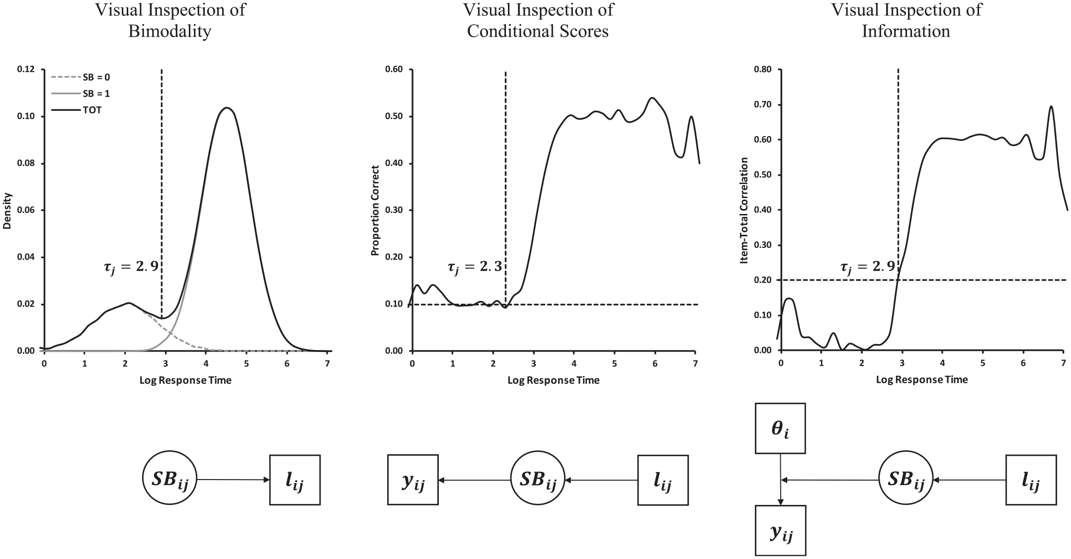
Upper panels = examples for procedures for setting response time thresholds based on artificial data. Lower panels = Graphical depiction of conceptual ideas underlying the procedures for setting response time thresholds.
A second approach combines response times with item responses (correct vs. incorrect), which are denoted as
A third method assumes that disengaged responses do not reflect proficiency (i.e., they are uninformative) (Wise, 2019). The method uses response times and correlations of item responses with provisional proficiency estimates (denoted as
Wise (2019) suggested a method in which the VICS and the VII procedures are combined. Conceptually, in the combined VICS–VII method, success rates and item information are simultaneously considered as outcomes of response engagement, whereas response times serve as predictors of engagement (Figure 1). A different possibility of combining some aspects of the VIB, the VICS, and the VII methods is to consider response times, success rates, and item information as indicators of engagement.
IRT Models for Response Engagement
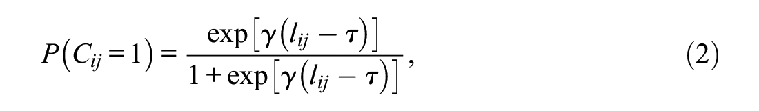
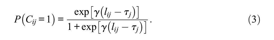
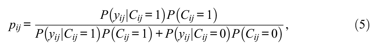
IRT models for response engagement build upon assumptions that parallel some assumptions of the VICS (the proportion of correct disengaged responses corresponds to the chance level) and the VII procedures (disengaged responses are not related to proficiency). The IRT models considered here recur on one dichotomous latent class variable
In the IRT models, the probability of a correct response is structured as

where
When the latent class variable is replaced with the SB-index, the structure corresponds to the effort-moderated IRT model of Wise and DeMars (2006), which estimates the IRT parameters and the individuals’ proficiency levels solely on the basis of responses that, through the use of threshold procedures, have been classified as engaged. The IRT models for response engagement enable researchers to bypass the cumbersome procedures of classifying the engagement status of each item response (Figure 1) and make it possible to deal with responses for which the engagement status cannot be univocally classified.
Similar to the procedures for setting response time thresholds, different kinds of IRT models for response engagement have been suggested that treat response times either as indicators or as predictors of the engagement states. The most commonly used IRT models (Ulitzsch et al., 2020; Wang & Xu, 2015; Wang et al., 2018) combine Schnipke and Scrams’s (1997) mixture model for response times with an IRT part and consider both response times and item responses as being influenced by the class variable. Therefore, we will refer to this group of models as independent latent class IRT (ILC-IRT) models. In a second type of mixture IRT models, the within-individual latent class variable is treated as a dependent variable that is predicted by response times (e.g., Pokropek, 2016). We will refer to this group of models as dependent latent class IRT (DLC-IRT) models.
DLC-IRT Models
DLC-IRT models where response times are used as predictors of response engagement have not often been used in practice. An exception is a model suggested by Pokropek (2016). In the following, we review this model and suggest some extensions to increase its flexibility.
DLC-IRT Models with Single-Level Relationships
Pokropek (2016) suggested a DLC-IRT model in which engagement states are predicted by within-individual level response times. Because relationships between response times, response engagement, and item responses are located solely on one level in Pokropek’s (2016) model, we refer to this type of model as a DLC-IRT model with single-level relationships (DLC-SL-IRT).
In contrast to Pokropek’s (2016)’s original model, we use log-transformed predictors, and we start with a slightly different but statistically equivalent parameterization. In this setup, the probability of an engaged response is expressed as
where
Pokropek’s (2016) model implies that within an individual i, a response to item j is more likely to be engaged than a response to another item k when
Item-specific thresholds
The DLC-SL-IRT model is sketched as a schematic path diagram in Figure 2. Response engagement is specified as a within-individual latent class variable
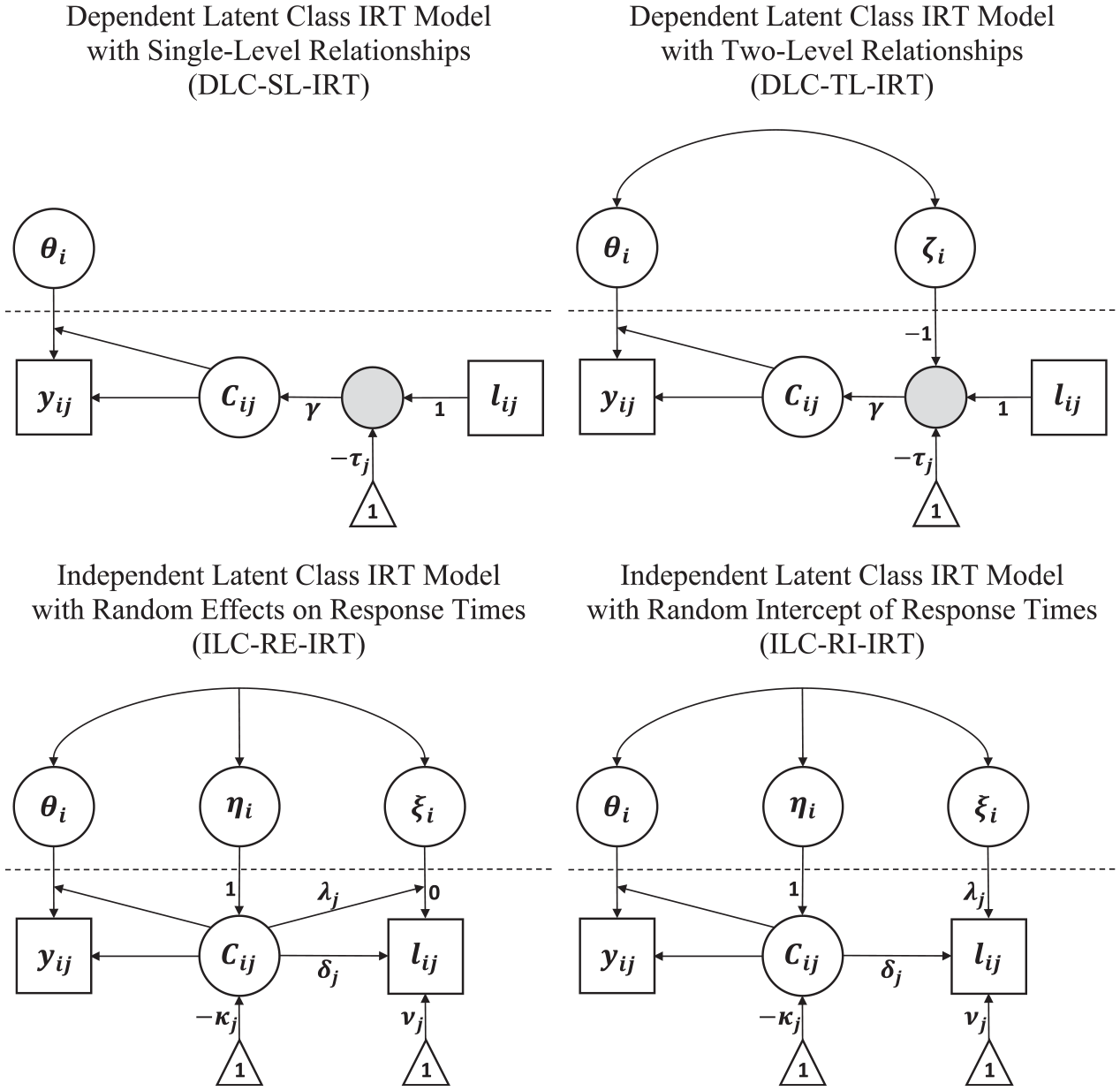
Schematic representation of different IRT models for response engagement. The dotted horizontal line separates the within-individual (lower part) from the between-individual (upper part) level of analysis. Gray filled circles represent node variables that are functions of other observed and latent variables. Triangles are used to indicate intercepts and thresholds.
DLC-IRT Models with Two-Level Relationships
The DLC-SL-IRT model implies that for each individual, the proportion of engaged responses can be fully explained by their item-specific log response times. This is because the model does not include between-individual differences in the latent class variable. However, Pokropek (2016) (see also Rios et al., 2017) noted that when between-individual differences that are conditional on response times exist in the proportion of engaged responses and these are correlated with proficiency, proficiency estimates are likely to be biased. From a conceptual point of view, such relationships are plausible. More proficient individuals have been found to need less time to complete an item conscientiously (e.g., Goldhammer et al., 2013), which means that, for such individuals, a response to item j that is given slightly below the response time threshold
In the DLC-TL-IRT model, we represent the impact of response times as
where
Figure 2 includes a graphical depiction of the DLC-TL-IRT model. The model extends the DLC-SL-IRT model by including the between-individual level threshold disturbance
Posterior Engagement Probabilities in DLC-IRT Models
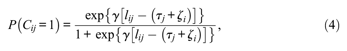
Equations (3) and (4) refer to the probability of an engaged response that are expected on the basis of response times and, therefore, do not provide a full insight into the probability that a response was actually engaged. To better understand the classification of responses in DLC-IRT models, it is instructive to consider the posterior probability of individual i’s response to item j being engaged, which we refer to as
where
Interim Summary of DLC-IRT Models
In DLC-IRT models, the meaning of the latent class variable is defined by the item responses, so that disengaged responses have a solution probability that corresponds to the chance level of success and are not related to proficiency. Response times are used as predictors of latent class membership, which means that response times are the main source of information used to separate engaged from disengaged responses. In the typical case of a low chance level of success, the posterior engagement probabilities in DLC-IRT models reduce the contribution of wrong responses coupled with fast response times in the estimation of IRT item parameters and proficiencies.
Therefore, DLC-IRT models are very similar to the combined ICS-VII procedure for setting response time thresholds (Figure 1). Of the two DLC-IRT models, the DLC-SL-IRT model is most similar to the VICS-VII procedure because it assumes that the response times contain all information necessary for predicting the engagement status of item responses. The DLC-TL-IRT model relaxes some restrictive assumptions, namely, that response times unequivocally predict the engagement status of each response (random threshold) and that conditional on response times engagement is not related to proficiency (correlation between random threshold and proficiency).
ILC-IRT Models
In ILC-IRT models, response times are considered to be indicators of response engagement. The basis of the most common type of ILC-IRT model was laid out by Schnipke and Scrams (1997). Their approach was extended by Wang and Xu (2015), Wang et al. (2018), and Ulitzsch et al. (2020), 1 who incorporated item responses into the models by using the structure shown in Equation (1) and imposing a similar structure on response times:

ILC-IRT models include an additional latent variable

for engaged responses and to

for disengaged responses. The tilde over the intercepts (
ILC-IRT models differ in how the class probabilities are expressed. Ulitzsch et al. (2020) provided the most comprehensive parameterization, which corresponds to
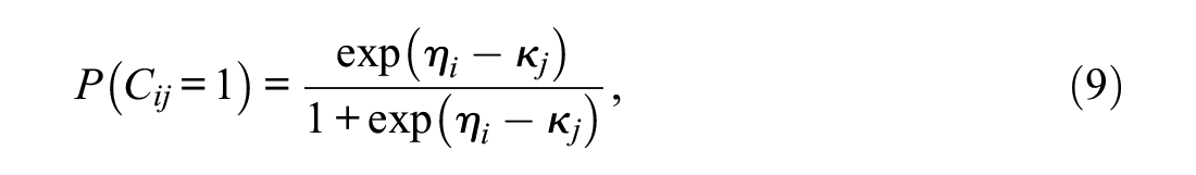
where
ILC-IRT models that include the
ILC-IRT Models With Random Effects of Response Engagement
Up until today, applications of ILC-IRT models have employed a constrained version of the structure provided in Equations (7) and (8). For engaged responses (Equation 7), the
The restrictions imposed on disengaged response times offer a substantive and a statistical interpretation of
To outline the random effect interpretation, we express the effect of

where
Figure 2 includes a schematic path diagram of the ILC-RE-IRT model. The latent class variable reflects the between-individual component
ILC-IRT Models with Random Intercepts of Response Engagement
The assumption that disengaged response times do not reflect typical time expenditure could be questioned when items elicit time-consuming actions even when responses are disengaged. For example, many items contain long reading passages, figures, and tables that require examinees to spend some time even if they examine the material only superficially. In addition, items that have an open response format require examinees to write down an answer, which is more time-consuming than randomly crossing one response option for a multiple choice item (Wise, 2019). In such cases, it is reasonable to assume that both engaged and disengaged response times depend on individuals’ typical time expenditure.
This assumption can be incorporated into ILC-IRT models by allowing the loadings

Here, the
The structure of ILC-RI-IRT models that also include
Posterior Engagement Probabilities in ILC-IRT Models
In ILC-IRT models the posterior engagement probabilities
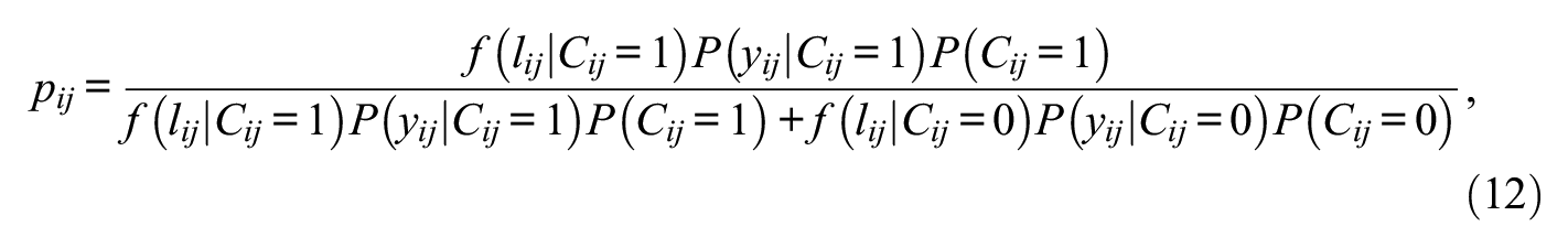
where
Typically, the means of disengaged responses are lower than the means of engaged responses. Therefore, long response times might be expected to be more typical for the engaged than the disengaged state (i.e., a higher PDF in the engaged than in the disengaged response time distribution). However, when the residual variance
Interim Summary of ILC-IRT Models
In ILC-IRT models, responses and response times jointly define the meaning of the latent class variable. Engaged item responses are assumed to be indicative of proficiency and to be accompanied by a specific distribution of response times. In contrast, disengaged responses are assumed to not reflect proficiency and to be accompanied by a different distribution of response times.
We presented two alternative ways of specifying ILC-IRT models for response engagement. The commonly used ILC-RE-IRT models (Ulitzsch et al., 2020; Wang & Xu, 2015; Wang et al., 2018) specify the relationships of the latent class variable with response times by means of a random effect regression, whereas ILC-RI-IRT models replace the random effect with a random intercept. These two specifications imply a different definition of typical time expenditure, so that
ILC-IRT models are conceptually related to the VIB method (Wise, 2015), but this connection is not as close as the one between DLC-IRT models and the VICS-VII method. Clearly, continuous response time variables carry more information than categorical item responses, so that latent class membership is more strongly determined by response times than by item responses (Wang & Xu, 2015). However, ILC-IRT models also account for item responses, whereas the VIB method does not. In addition, the VIB procedure aims to separate fast disengaged responses from engaged responses on the basis of a response time threshold (monotonic relationship), whereas ILC-IRT IRT models allow for more complex relationships between response times and engagement.
DLC-IRT versus ILC-IRT Models
DLC-IRT and ILC-IRT models provide two different ways to include response times in IRT models for response engagement. Table 1 summarizes how response times are used in the different models considered in this article. In ILC-IRT models, response times are specified as reflections of response engagement, whereas in DLC-IRT models, response engagement is predicted by the individuals’ response times. Therefore, DLC-IRT and ILC-IRT models differ in how dependencies between item responses and response times are modeled. DLC-IRT models consider the distribution of item responses conditional on response times, which means that they take response times as given, without incorporating specific assumptions about their distribution. In contrast, in ILC-IRT models, the joint distribution of item responses and response times is modeled on the basis of assumptions about the structure and the distribution of response engagement and response times. These assumptions make it possible to estimate complex relationships between response engagement and response times that could be non-monotonic (Equation 12) and could differ in strengths between items (Equations 10 and 11). In contrast, in DLC-IRT models, item-specific response times are assumed to have monotonic relationships of equal strength with response engagement. Given the fundamental differences between ILC-IRT and DLC-IRT models, decisions in favor of one type of model should be based on substantive considerations. Decisions cannot rely on goodness-of-fit indices based on the model likelihood (e.g., Akaike information criterion and Bayesian information criterion) because DLC-IRT and ILC-IRT models consider different aspects of the data. However, such indices can be used to decide between variants of either type of model.
Summary of the Key Aspects of the Treatment of Item Response Times in Dependent Latent Class (DLC-IRT) and Independent Latent Class (ILC-IRT) Models for Response Engagement.
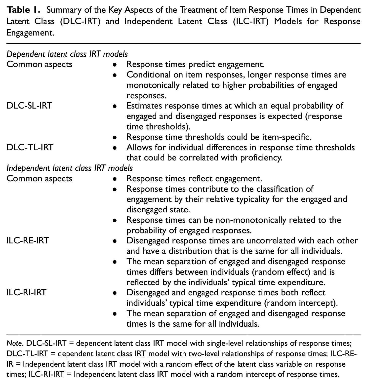
Note. DLC-SL-IRT = dependent latent class IRT model with single-level relationships of response times; DLC-TL-IRT = dependent latent class IRT model with two-level relationships of response times; ILC-RE-IR = Independent latent class IRT model with a random effect of the latent class variable on response times; ILC-RI-IRT = Independent latent class IRT model with a random intercept of response times.
The most important aspect to consider when deciding on a model type is the assumptions about the role of response times and the definition of response engagement. DLC-IRT models take a perspective that is typical for the rapid guessing literature, according to which response engagement can be expressed as a monotonic function of response times (the longer the response time, the more likely it is that the response is engaged; Wise, 2019). Furthermore, in this stream of research, it is not common to make structural and distributional assumptions about response times. Therefore, researchers favoring the perspective pursued in research on rapid guessing might find DLC-IRT models to be most attractive. Indeed, DLC-IRT models provide many benefits compared to the typically time-consuming and cumbersome two-step procedures employed in this field (threshold-based classification of response engagement followed by the IRT analyses of responses classified as engaged). DLC-IRT models are one-step procedures that are easy to apply. Here, response time thresholds are estimated within the model, and the model-implied posterior engagement probabilities are accounted for in the estimation of IRT item parameters and individual proficiency levels. Furthermore, DLC-IRT models have the appealing feature that they can examine individual differences in response time thresholds (DLC-TL-IRT), whereas this is not possible on the basis of traditional methods.
ILC-IRT models contain the key ingredients of van der Linden’s (2007) speed-accuracy IRT model, which is frequently used in psychometrically inspired research. This model is based on the assumption that individuals have their own typical working speed (or typical time expenditure), which they maintain over the course of a test. One key research question employed on the basis of this model refers to the relationships between proficiency and typical time expenditure (e.g., Goldhammer et al., 2013). Disengaged item responses violate the constant time expenditure assumption, which means that ILC-IRT models can be seen as extensions of the speed-accuracy IRT model that account for such violations. As such, ILC-IRT models are a suitable choice when researchers are interested in the relationships between proficiency and typical time expenditure and wish to account for disengaged responses defined by atypical response times. In this vein, the two variants of ILC-IRT models, is whether the log response times’ loadings interact (ILC-RE-IRT) or do not interact (ILC-RI-IRT) with the latent class variable, might prove useful in deriving accurate representations of individuals’ typical time expenditure and engagement states.
The MM-IRT for Response Engagement
In this section, the MM-IRT framework, which allows the previously presented IRT models to be estimated with Mplus (Muthén & Muthén, 2017), is introduced. We first describe how the input data are structured and then move to the specification and estimation of DLC-IRT and ILC-IRT models. The section ends with an illustration of the framework.
Data Setup
IRT models can be formulated and estimated as multilevel models with item responses organized in a long format (e.g., Van Den Noortgate et al., 2003). This setup can be extended to MM-IRT models by including an item-level latent class variable (e.g., Asparouhov & Muthén, 2008; Pokropek, 2016). However, in our experience, the estimation of MM-IRT models on the basis of a long data format is computationally very demanding because the models require the estimation of a large number of interactions. As a solution to this problem, we propose a rearrangement of the input data that greatly speeds up the estimation times when employing MML estimation.
In our setup, the item responses are organized in a diagonal format. Each individual i’s item responses are represented in a matrix
Example of a Data Array for One Individual in the Diagonal Format. Variables in the Columns are Indexed by Item (k = 1, 2, …, K with K = J). The Example includes Two Alternative Organizations of Log Response Times as Used in DLC-IRT and ILC-IRT Models.
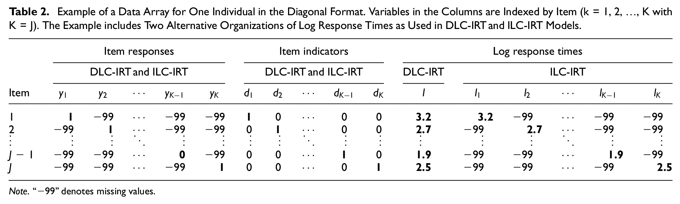
Note. “−99” denotes missing values.
Specification of IRT Models for Response Engagement in the MM-IRT Framework
Specification of the IRT Part for Item Responses
We first outline the specification of the IRT part that is used to model item responses in all models. In our MM-IRT framework, item responses are represented by a 2PL model that provides a good compromise between flexibility and parsimony and is well suited for the open responses considered in this article.
To include the 2PL part in the MM-IRT framework, we specify the item responses to be located on the within-individual level and the proficiency variable to be located on the between-individual level. For engaged item responses, the 2PL structure is parameterized as
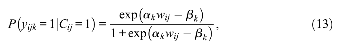
where

which means that the proficiency variable
For disengaged responses, the success probability does not depend on proficiency, and the probability of a correct response corresponds to the chance level of success. In this case, Equation (13) is altered to
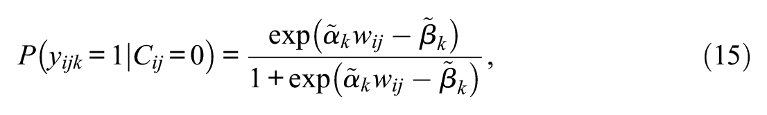
with
Specification and Estimation of DLC-IRT Models
The estimation of the variants of DLC-IRT models recurs on alternative but statistically equivalent parameterizations of Equations (3) and (4). We begin with the more complex DLC-TL-IRT model because the DLC-SL-IRT model is a constrained version thereof. In the DLC-TL-IRT model the latent class variable is specified to depend on item response times that are organized in a long format (Table 2) and on the K = J item indicators via a logistic regression:
where
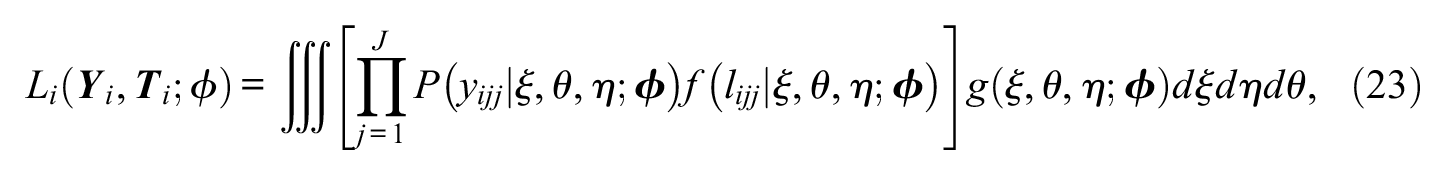
The DLC-IRT models can be estimated by MML through the EM algorithm. MML estimation follows from the procedures outlined by Vermunt (2003). The log likelihood to be maximized is given by
where
As only the diagonal entries (j = k) of
where individual responses are indexed as
Specification and Estimation of ILC-IRT Models
The estimation of ILC-IRT models in the MM-IRT framework requires response times to be organized in a diagonal format (Table 2). On the basis of this data setup, the measurement structure of typical time expenditure is expressed by modifying Equation (7) to

and Equation (8) to

The index k in Equations (19) and (20) replaces the item index j, which means that

where the between-individual random effect variable
The MML estimation of ILC-IRT models is more challenging. The log likelihood to be maximized is given by (e.g., Vermunt, 2008)
which means that, in these models, we consider the joint distribution of item responses and response times that have a probability density that corresponds to
where
Illustrative Application to the PIAAC Data
Illustrative Data
PIAAC is an international large-scale assessment of proficiencies in adults. Here, we consider the literacy test administered in the French-speaking samples (France and Canada). We chose this sample because previous research suggests that it exhibits a typical level of disengagement (Goldhammer et al., 2016), and it offers a sample size that is large enough to estimate the models. In PIAAC, a two-stage booklet design is used. In the first stage, examinees are randomly assigned to one of three booklets. Each booklet has a different level of difficulty and consists of nine items. In stage two, individuals are then assigned to one of four different booklets that contain 11 items each. All items have an open response format, which means that the success probability of disengaged responses can be expected to be essentially zero. In order to derive a sample with a decent number of items without introducing additional complications caused by the design, we selected a subgroup of examinees who had worked on a specific combination of stage-one and stage-two booklets (“low” and “intermediate one”). To keep the examples simple, we used only examinees who answered all 20 items (N = 637).
Model Specification and Estimation
All IRT models for response engagement were estimated with Mplus 8.4 (Muthén & Muthén, 2017) using the accelerated EM algorithm and employing 15 integration points per dimension. As models that include latent class variables could be prone to local optima (Lubke & Muthén, 2005), we employed multiple random starting values to check whether the best log likelihood had been replicated. The Mplus input files for all models are provided in the Supplemental Material.
In our application of DLC-IRT models, the
Model-Data Fit
Decisions between DLC-IRT and ILC-IRT models cannot be based on information criteria, but these indices can be used to examine the merits of accounting for response engagement by comparing the fit of each type of IRT model for response engagement with the fit of a suitable reference model. We chose the 2PL IRT model as a reference for the DLC-IRT models, whereas ILC-IRT models were compared to van der Linden’s (2007) speed-accuracy IRT model (denoted as 2PL + RT). Information criteria were furthermore used to examine the different specifications of each type of IRT model for response engagement. Table 3 summarizes the goodness-of-fit statistics of all IRT models. The DLC-SL-IRT model fitted the data better than the 2PL model, and the fit was further improved by extending the model to the DLC-TL-IRT model. Compared to the 2PL + RT model, the model-data fit was improved by the ILC-IRT models. The ILC-RI-IRT model fitted clearly better than the ILC-RE-IRT model.
Goodness-of-Fit Measures of IRT Models for Response Engagement.
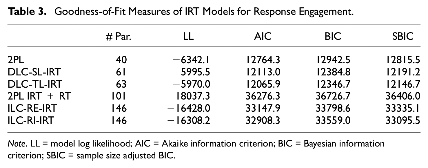
Note. LL = model log likelihood; AIC = Akaike information criterion; BIC = Bayesian information criterion; SBIC = sample size adjusted BIC.
Response Time and Response Engagement
In both DLC-IRT models the process discrimination parameters documented a strong effect of response times (DLC-SL-IRT:
Estimated Response Thresholds in DLC-IRT Models and Engagement Difficulties in ILC-IRT Models, and Estimated Proportion of Engaged Responses (Average Posterior Latent Class Probabilities).
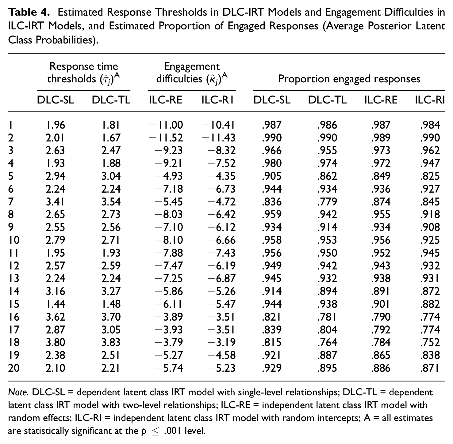
Note. DLC-SL = dependent latent class IRT model with single-level relationships; DLC-TL = dependent latent class IRT model with two-level relationships; ILC-RE = independent latent class IRT model with random effects; ILC-RI = independent latent class IRT model with random intercepts; A = all estimates are statistically significant at the p ≤ .001 level.
In the ILC-IRT models, the relationships of response engagement with response times are represented by the separation of engaged and disengaged response time distributions. The upper panel in Figure 3 reports the results of the ILC-RE-IRT model on the basis of the engaged and disengaged response time intercepts and the regions around the intercepts that comprised 80% of the values (±1.282 residual standard deviations). Therefore, in the case of engaged responses, the vertical bars indicate the region in which the response times of individuals with an average value of
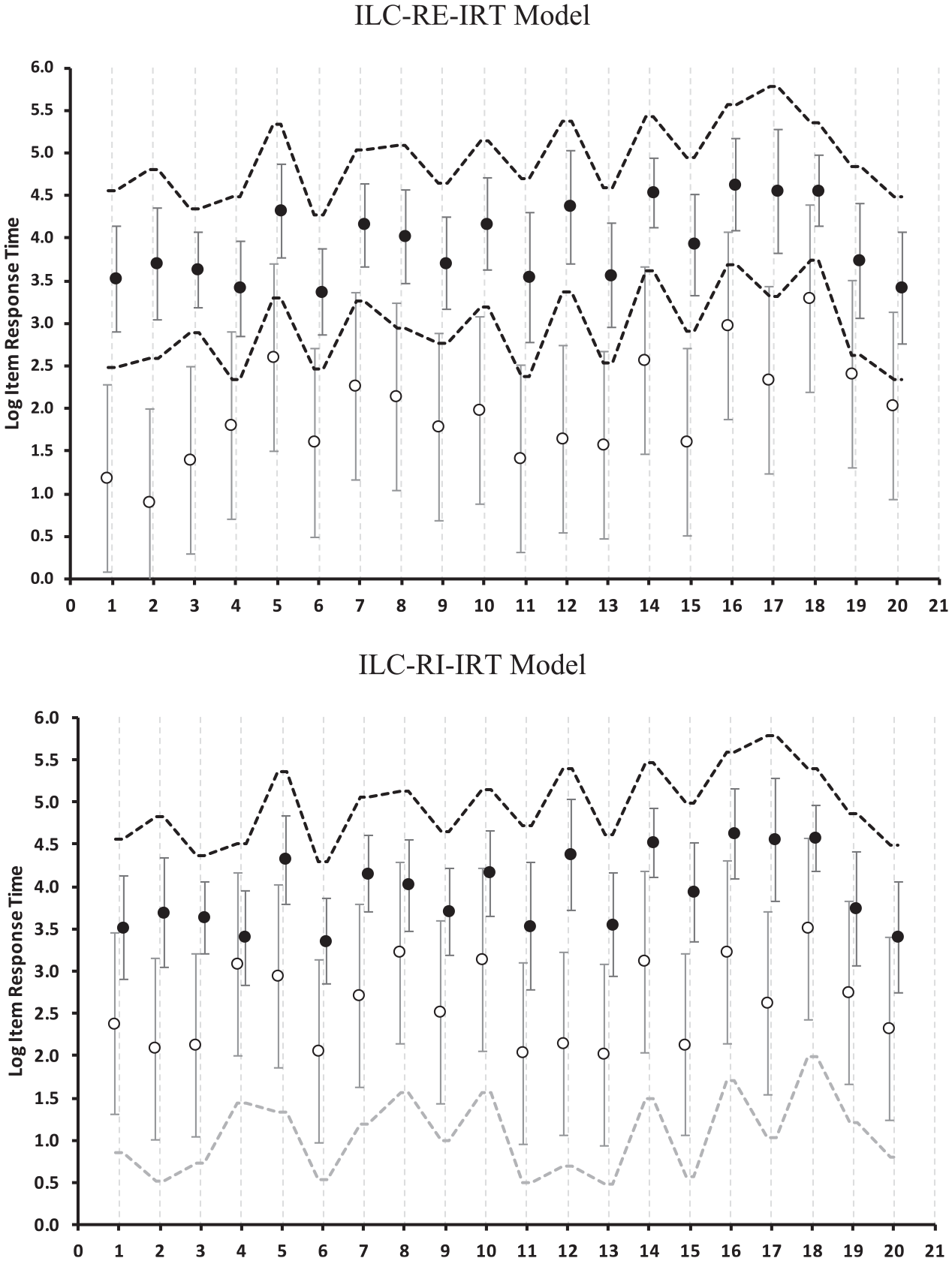
Separation of log response times of engaged and disengaged responses provided by the independent latent class IRT model with random effects (ILC-RE-IRT) and the independent latent class IRT model with random intercepts (ILC-RI-IRT). Circles represent intercepts of engaged (filled black) and disengaged (open) log response times. Vertical bars represent the range between the 10th and 90th percentile of the residual distributions around the intercepts. Dotted lines visualize the impact of individual differences in typical time expenditure.
The lower panel in Figure 3 describes the response time distributions given by the ILC-RI-IRT model. Because the separation of engaged and disengaged response times is specified to be the same for all individuals, dotted lines that indicate the impact of the random intercept
The posterior engagement probabilities given by the ILC-IRT models are reported together with the engagement difficulties in Table 4. Overall, the engagement difficulty parameters and the posterior probabilities were similar in both ILC-IRT models. However, the ILC-RI-IRT model indicated a lower proportion of engaged responses (89.0% vs. 90.8%). This difference was reflected in the larger overlap of response time distributions in the ILC-RI-IRT model (Figure 3), which means that, in this model, relatively long response times were more likely to be classified as disengaged than in the ILC-RE-IRT model.
Both ILC-IRT models provided very similar results with respect to the latent characteristics: They estimated a large variability in engagement propensities (ILC-RE-IRT:
Adjustments of IRT Item Parameters
The estimates of the IRT item parameters are summarized in Figure 4. Compared to the 2PL model, both DLC-IRT models estimated lower item discriminations, but discriminations were slightly lower in the DLC-TL-IRT model. This result suggested that the variability in proficiencies represented by the 2PL model might be inflated by individual differences in response engagement. Figure 4 includes estimates of the item difficulties (i.e.,
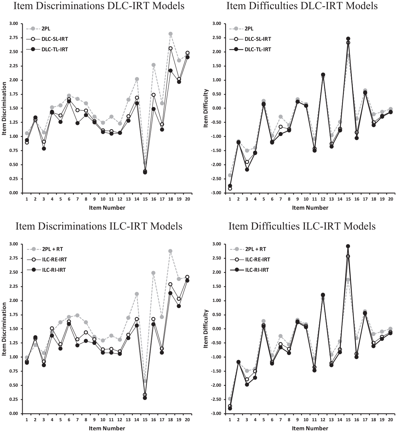
Estimates of item discriminations and difficulties derived from DLC-IRT and ILC-IRT models. Results from a conventional 2PL IRT model and a 2PL IRT model including a congeneric measurement model for time expenditure based on log response times (2PL + RT) as a comparison standard.
Adjustments of Proficiency Estimates
The adjustments of the proficiency estimates provided by the IRT models for response engagement relative to the 2PL model were based on EAP estimates of
Figure 5 presents the scatter plots of the EAP
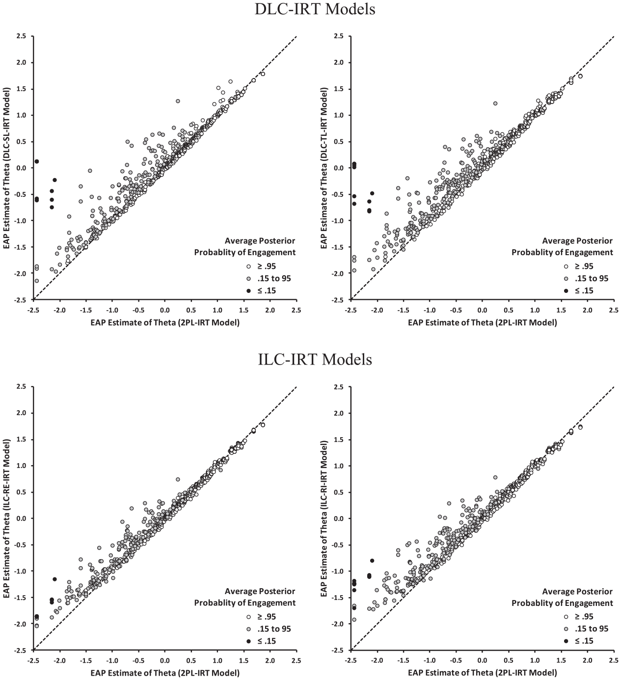
Scatter plots of EAP proficiency estimates provided by the 2PL IRT model (x-axis) and by equated EAP proficiency estimates provided by the DLC-IRT (y-axis in upper panels) and the ILC-IRT models (y-axis in lower panels) for individuals with different levels of engagement (average posterior probabilities of engagement).
Both ILC-IRT models provided proficiency estimates adjusted for response engagement that differed from the estimates of the 2PL IRT model (Figure 5). The marginal distribution of EAP
Summary
All IRT models for response engagement supported the suspicion that the PIAAC literacy assessment was affected by disengaged responses (Goldhammer et al., 2016). In addition, the results indicate that the details of the models’ specifications matter. The preferred DLC-TL-IRT and ILC-RI-IRT models provided stronger adjustments of IRT item parameters and proficiency estimates than the DLC-SL-IRT and ILC-RE-IRT models. However, the information criteria do not tell whether the DLC-TL-IRT or the ILC-RI-IRT model should be chosen as the final model. Nevertheless, we can conclude that DLC-IRT and ILC-IRT models fit the data better than the reference models that do not separate response states and that, within each type of IRT model for response engagement, one parameterization fits the data better than the other. We do not consider this aspect of model selection to be problematic because, in real applications, researchers should decide on one type of IRT model for response engagement on the basis of the perspective they have on response times.
Interestingly, in the present applications, the results pertaining to the item responses and the proficiencies provided by these two preferred DLC-IRT and ILC-IRT models were remarkably similar. Given the fundamental differences between the two types of models, such results should not be taken for granted. Indeed, a closer look at the relationships between response times and posterior engagement probabilities revealed non-monotonic relationships in the ILC-RI-IRT model (i.e., some responses associated with very long response times were classified as disengaged; details available upon request). However, in the present application, only a small number of responses was affected by the non-monotonic relationships, which means that the model estimates were not overly affected by this phenomenon.
Summary and Discussion
IRT models for response engagement are tools that allow item responses and response times to be considered simultaneously, while avoiding the necessarily error-prone procedures for classifying the engagement status of item responses. IRT models for response engagement build upon different assumptions, which means that different IRT models can give different results when they are applied to the same data. Therefore, the objectives of the present article were: (1) to outline the rationale of the commonly employed methods for setting response time thresholds, (2) to describe the assumptions they share with different types of IRT models for response engagement, (3) to suggest model extensions that increase the IRT models’ flexibility, and (4) to provide a flexible MM-IRT framework that makes it possible to estimate various IRT models for response engagement.
Types of IRT Models for Response Engagement
We have delineated that IRT models for response engagement and observed variable procedures are built on common ideas, and we have proposed the distinction between ILC-IRT models, which consider response times as indicators of response engagement, and DLC-IRT models, in which response times serve as predictors of engagement.
Up until today, most IRT models for response engagement belong to the class of ILC-IRT models in which response engagement is defined jointly on the basis of item responses and response times. However, because the continuous log response times carry more information (Wang & Xu, 2015), they are likely to determine the classification of response engagement more strongly than item responses. As such, ILC-IRT models are connected to the VIB method, which uses only response times, but this connection is loose because ILC-IRT models use the complete data and are based on additional structural assumptions. In our view, ILC-IRT models can be best understood as extensions of van der Linden’s (2007) speed-accuracy IRT model, which make it possible to account for violations of the constant time expenditure assumption due to disengaged responses. Disengaged item responses are specified to not depend on proficiency and to be accompanied by response times that stem from a different distribution than that of engaged responses. In ILC-IRT models response times contribute to the classification of response engagement according to their typicality for each engagement state (Equation 12), which means that these models could classify very slow responses as disengaged responses. From the perspective of the typical time expenditure assumption, such kinds of non-monotonic relationships make sense because both fast and very slow responses could be considered to be atypical and disengaged.
The variants of ILC-IRT models presented here use response times differently for classifying response engagement. ILC-RE-IRT models assume that engaged response times differ from an unstructured reference distribution, which means that the more strongly an item’s response time deviates from the reference distribution, the more likely it is that the response is engaged. In contrast, ILC-RI-IRT models state that both engaged and disengaged responses reflect individuals’ typical time expenditure and that the separation between engaged and disengaged response times is the same for all individuals. As shown in the exemplary application, the variants of ILC-IRT models can provide different results. Therefore, researchers need to carefully consider which type of ILC-IRT model is more plausible. The ILC-RI-IRT model might be a better choice when tests consist of items that require nontrivial time expenditure even when responses are not engaged.
By relating response times to response engagement based on the theoretical consideration that faster responses can—with higher certainty—be considered to be disengaged, and without recurring on assumptions about the structure of response times, DLC-IRT models closely mirror the perspectives taken in the research on rapid guessing behavior. Therefore, although DLC-IRT models have not attracted much attention in the literature (but see Pokropek, 2016), we believe that they have much to offer. In this article, we have proposed two extensions of Pokropek’s (2016) DLC-IRT model that both include item-specific response time thresholds that are based on a rationale similar to that of the combined VICS and VII methods (Wise, 2019). As such, DLC-IRT models can be conceived as model-based, one-step procedure counterparts of the VICS-VII procedure.
Of the two variants of DLC-IRT models presented, the DLC-SL-IRT model is closest to the typical approach of classifying each individual’s response engagement on the basis of the same response time thresholds. The DLC-TL-IRT is an extension thereof that allows for individual differences in response time thresholds that could be correlated with proficiency. The failure to include such a component in DLC-IRT models has been discussed as a potential source of bias (Pokropek, 2016; Rios et al., 2017), and we have demonstrated that including individual differences in response time thresholds could indeed affect item parameter and proficiency estimates.
Taken together, the DLC-IRT and ILC-IRT models are conceptually different and fit to different theoretical perspectives of response times as reflections or causes of response engagement. Therefore, decisions in favor of one type of model should optimally be theoretically justified, or the substantive considerations underlying the decision should at least be clearly laid out. Such explanations should be self-evident in research. In the present context, they gain additional importance because DLC-IRT and ILC-IRT models use the input data in different ways so that decisions cannot be guided by information criteria.
The MM-IRT Framework
A further objective of this article was to describe an MM-IRT framework that allows a variety of IRT models for response engagement to be estimated by means of the Mplus software. Our framework is based on a diagonal arrangement of the latent variables’ indicators. This setup combines the strengths of traditional wide and long data formats. An advantage of the wide data format is that all measurement parameters can differ between indicators and latent classes. However, this flexibility comes at the price of requiring a large number of latent class variables, which limits the application of IRT models for response engagement to rather small numbers of items (e.g., Molenaar et al., 2016). In the long data format, multiple latent class variables can be replaced with one class variable located on the within-individual level. The measurement parameters of the indicators of the latent continuous variables are modeled by the effects of the item indicators and their interactions with the latent class variable (Pokropek, 2016). The drawbacks of this arrangement are that it is less flexible in modeling residual structures and that the estimation of item-specific discrimination and loading parameters is computationally demanding. The diagonal data arrangement provides the same flexibility as the wide format and allows a large number of items to be included in the models, while still supporting computationally efficient MML estimation.
The MM-IRT framework provides great flexibility because, in principle, all parameters can be specified to be item-specific. The IRT models applied in this article include fewer constraints than the models employed in the literature (e.g., Ulitzsch et al., 2020), and the constraints can be further relaxed. An important aspect of the MM-IRT framework is that it is not limited to item response times, and it allows alternative predictors or indicators of response engagement to be incorporated into IRT models for response engagement. This feature makes it possible to investigate the utility of other within-individual variables, such as interest ratings (e.g., Lindner et al., 2019) or repeating response patterns (e.g., Cui, 2020), as alternative or additional predictors or indicators of response engagement in DLC-IRT and ILC-RIT models, respectively. Similarly, the proposed models can be extended by between-individual variables, which makes it possible to study their relationships with individual differences in thresholds or engagement (e.g., Nagy et al., 2019). These possibilities should be explored in more detail in further research.
Further Research
The models presented here are, in some respects, more constrained than some other models suggested in the literature. The IRT model applied to engaged responses does not include pseudo-guessing parameters, which might be desired in the case of multiple choice items. We plan to explore this modeling option in future studies.
A concern in the context of ILC-IRT models could be the assumption that item-specific engagement states are conditionally independent. An alternative is to consider that item-specific engagement states depend on previous states. Molenaar et al. (2016) suggested a model in which response processes are modeled by a hidden Markov process, but their model has not been applied to response engagement yet. Future research could investigate possibilities to include such dependencies in IRT models for response engagement. However, an interesting line of research would be to study whether serial dependencies can be accounted for by means of DLC-IRT models that are computationally less demanding. In this vein, more research could be devoted to DLC-IRT models to increase their flexibility, for example, by including item-specific effects of response times and accounting for measurement error in response times (Molenaar & de Boeck, 2018).
Conclusion
The MM-IRT framework makes it possible to specify and estimate a variety of ILC-IRT and DLC-IRT models that extend the arsenal of latent variable models for response engagement. Furthermore, the MM-IRT framework makes the IRT models for response engagement accessible to applied researchers. Indeed, as shown in the Supplemental Material., the Mplus input code for specifying the models is not complicated. We hope that the ideas and the procedures outlined here will prove useful to researchers studying the impact of response engagement (Wise, 2015) and will stimulate research that extends our knowledge about test-taking motivation (e.g., Nagy et al., 2018).
Supplemental Material
sj-docx-1-epm-10.1177_00131644211045351 – Supplemental material for A Multilevel Mixture IRT Framework for Modeling Response Times as Predictors or Indicators of Response Engagement in IRT Models
Supplemental material, sj-docx-1-epm-10.1177_00131644211045351 for A Multilevel Mixture IRT Framework for Modeling Response Times as Predictors or Indicators of Response Engagement in IRT Models by Gabriel Nagy and Esther Ulitzsch in Educational and Psychological Measurement
Footnotes
Declaration of Conflicting Interests
The author(s) declared no potential conflicts of interest with respect to the research, authorship, and/or publication of this article.
Funding
The author(s) received no financial support for the research, authorship, and/or publication of this article.
Supplemental Material
Supplemental material for this article is available online.
Notes
References
Supplementary Material
Please find the following supplemental material available below.
For Open Access articles published under a Creative Commons License, all supplemental material carries the same license as the article it is associated with.
For non-Open Access articles published, all supplemental material carries a non-exclusive license, and permission requests for re-use of supplemental material or any part of supplemental material shall be sent directly to the copyright owner as specified in the copyright notice associated with the article.