Overview of the winning approaches in BCI Controlled Robot Contest in World Robot Contest 2021: Calibration-free SSVEP

Abstract

Recently, steady-state visual evoked potential (SSVEP) has become one of the most popular electroencephalography paradigms due to its high information transfer rate. Several approaches have been proposed to improve the performance of SSVEP. The calibration-free scenario is significant in SSVEP-based brain–computer interface systems, where the subject is the first time to use the system. The participating teams proposed several effective calibration-free algorithm frameworks in the SSVEP competition (calibration-free) of the BCI Controlled Robot Contest in World Robot Contest 2021. This paper introduces the approaches used in the algorithms of the top five teams in the final. The results of the five subjects in the final proved the effectiveness of the approaches. This paper discusses the effectiveness of each approach in improving the system performance in the calibration-free scenario and gives suggestions on how to use these approaches in a real-world system.

1 Introduction

A brain–computer interface (BCI) offers people an alternative way to communicate with or control an external device. It directly measures the user’s brain activities and translates them into corresponding control signals for BCI applications [1]. Electroencephalogram (EEG) is the most popular input signal in BCIs due to its simplicity and low cost, which records electrical activities from the scalp [2]. There are several paradigms widely used in BCIs, e.g., P300 evoked potentials [3], motor imagery [4], and steady-state visual evoked potential (SSVEP) [5]. Compared with other paradigms, SSVEP enjoys more widespread adoption due to its high information transfer rate (ITR), short user training time, and ease of use. When the user stares at a target flickering at a frequency ranging from 3.5 to 75 Hz, the brain generates EEG signals at the target’s frequency at the same (or multiples of the) frequency [6]. Thus, it is easy to know which target the user is paying attention to by identifying the frequency information of the user’s current EEG signals.

Multiple frequency recognition approaches have been developed to improve the performance of SSVEP-based BCIs. They are divided into calibration-free and calibration-based approaches based on whether the calibration data are required. Calibration-free approaches are easy to implement and do not need any calibration data, e.g., canonical correlation analysis (CCA) [7], minimum energy combination [8], multivariate synchronization index [9], and Ramanujan periodicity transforms [10]. However, calibration-free approaches need a long stimulation duration to achieve high accuracy, leading to low ITR. To increase ITR when calibration data can be obtained, the SSVEP-based BCI system can use calibration-based approaches to construct specific templates and spatial filters for the subjects, e.g., extended CCA (eCCA) [11], modified eCCA (m-eCCA) [12], L1-regularized multiway CCA (L1MCCA) [13], task-related component analysis (TRCA) [14], task-discriminant component analysis [15]. These approaches improve the performance of SSVEP.

The high-performance of SSVEP helps develop the application of BCIs in visual spellers [12] and device controllers [16]. Figure 1 shows the workflow of a classical SSVEP speller used in the SSVEP competition (calibration-free) of the BCI Controlled Robot Contest in World Robot Contest 2021 (WRC2021). Figure 2 shows the detailed layout of the visual keyboard used in the speller. There are 40 targets (including 0–9, A–Z, comma, dot, space, and backspace) flickering at different frequencies ranging from 8 to 15.8 Hz with a frequency interval of 0.2 Hz and an initial phase interval of 0.5π. The user needs to stare at a target character, then EEG signals will be collected through the EEG headset and transmitted to a computer. When a sufficiently long EEG trial is collected for analysis, the algorithm will process the EEG trial and mine the frequency information. Finally, the target character will be shown on the screen.

Fig. 1

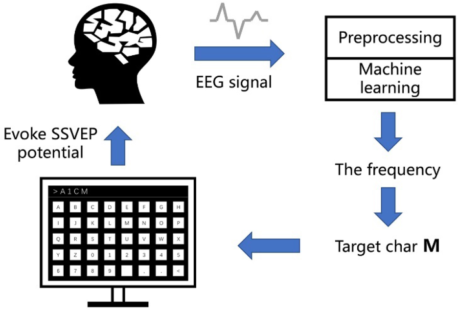
Workflow of an SSVEP speller.

Fig. 2

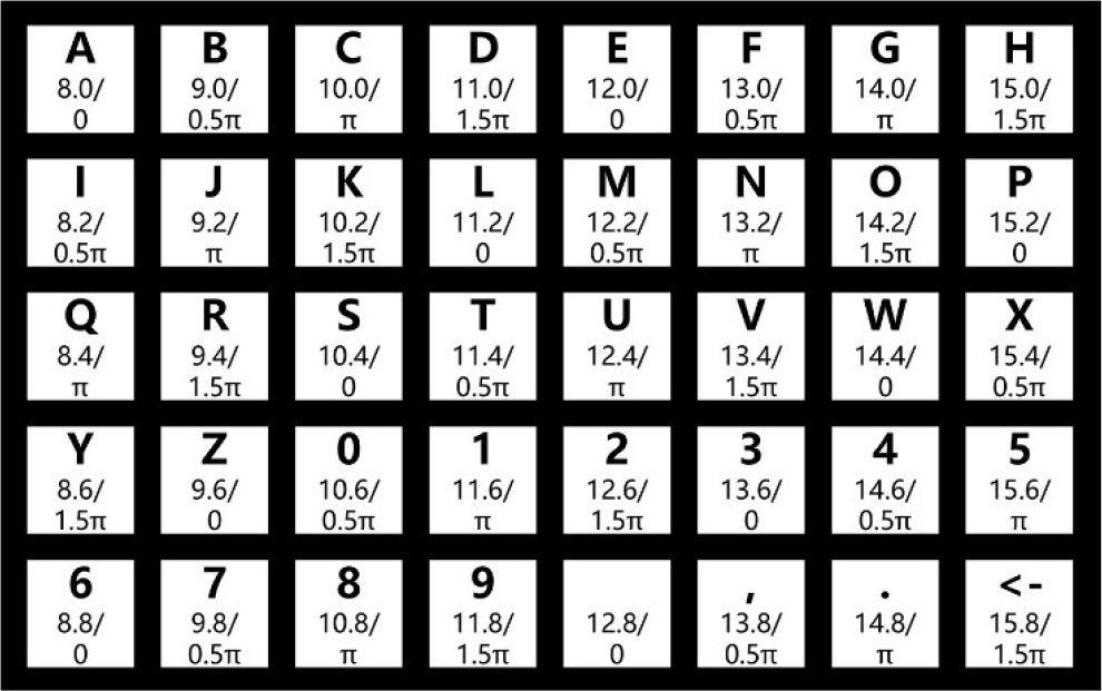
Stimulation interface used in the final. The two numbers below each character indicate its flickering frequency (Hz) and initial phase (in radius).

In this paper, we introduce the algorithms used by the top five teams (Hust-BCI, MuTouRen, CQU-faster, LuQiXiuZiJiaYouGan, and BrainStorm) in the final of the SSVEP competition (calibration-free) of WRC2021. We are from Hust-BCI. For simplicity, the algorithms of the five teams will be called Algo-H (Hust-BCI), Algo-M (MuTouRen), Algo-C (CQU-faster), Algo-L (LuQiXiuZiJiaYouGan), and Algo-B (BrainStorm). This paper aims to verify the performance of different algorithms in the calibration-free scenario.

The remainder of this paper is organized as follows. Section 2 introduces the five algorithms, including the preprocessing methods, frequency recognition approaches, and dynamic window framework. Section 3 presents the results of the five subjects in the final and verifies the approaches’ effectiveness on the benchmark dataset. Section 4 discusses the effectiveness of each approach. Finally, Section 5 presents the conclusion.

2 Methods

This section first introduces the experimental settings used in the competition. Then, we present the preprocessing methods used by the five teams and the frequency recognition approaches, including CCA [7], eCCA [11], TRCA [14], and the filter bank method [17]. Finally, we present the dynamic window framework used by all five teams and the differences in their implementation of this framework.

2.1 Preprocessing methods

All five teams used a 50-Hz notch filter due to the 50-Hz power line noise. Algo-H and Algo-L used a band-pass filter to remove the high and low-frequency noise. All teams extracted data 0.14 s after stimulus onset, because there is a latency [18] in the visual system.

In Algo-H, in addition to the above methods, we used image filtering denoising (IFD) proposed by Yan et al. [19] to denoise the EEG data. In IFD, the authors found that image filtering of SSVEP could not effectively remove the noise; thus, they proposed a reverse solution in which the SSVEP noise signal was obtained by image filtering, and the noise was subtracted from the original signal.

2.2 Canonical correlation analysis

Lin et al. [7] first used CCA to enhance the signal-to-noise ratio (SNR) of SSVEPs. CCA can be used to extract the underlying correlation between two multi-channel time-series [20]. The main idea of CCA is to obtain linear combinations for the two signals to maximize their correlation. Let $X\in {ℝ}^{N_c\times N_s}$ denote an EEG trial with N _c channels and N _s samples. Y _f is a sine–cosine reference signal for frequency f and phase ϕ _f , given as follows:

${\text{Υ}}_f=\left[\begin{array}{c}\sin \left(2\pi ft+{\varphi }_f\right)\\ \cos \left(2\pi ft+{\varphi }_f\right)\\ ⋮\\ \sin \left(2\pi nft+{\varphi }_f\right)\\ \cos \left(2\pi nft+{\varphi }_f\right)\end{array}\right],t=\frac{1}{f_{\text{s}}},\frac{2}{f_{\text{s}}},\cdots ,\frac{N_{\text{s}}}{f_{\text{s}}}$

1

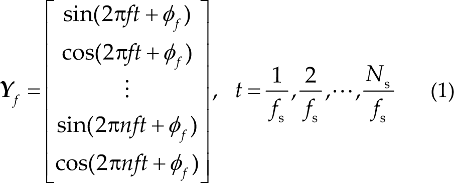
where f _s is the sampling rate, and n is the number of harmonics. The weight vectors W _X and $W_{y_f}$ can be computed by solving the following optimization problem:

$W_X,W_{Y_f}=\underset{W_X,W_{Y_f}}{argmax}\frac{E\left[W_X^{\text{T}}X{X}_f^{\text{T}}{W}_{Y_f}\right]}{\sqrt{E\left[W_X^{\text{T}}X{X}^{\text{T}}{W}_X\right]E\left[W_{Y_f}^{\text{T}}{Y}_f{Y}_f^{\text{T}}{W}_{Y_f}\right]}}$

2

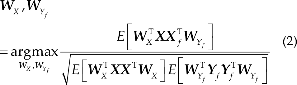
Then, the CCA correlation between X and Y _f can be computed by applying the Pearson’s correlation ρ to X ^T W _X and $Y_f^T{W}_{Y_f}$ .Let K be the number of targets (K = 40 in this paper). The stimulation frequency of the EEG trial is determined by solving the following optimization problem:

$f^{\ast }=\underset{f\in {\left\{f_i\right\}}_{i=1}^K}{\text{argmax}}\rho \left(X^{\text{T}}{W}_X,Y_f^{\text{T}}{W}_{Y_f}\right)$

3

2.3 Extended canonical correlation analysis

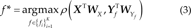
Extended canonical correlation analysis (eCCA) [11] computes the spatial filters using the subject-specific reference and the sine–cosine reference signals to improve the performance of the CCA-based method. Let ${\overline{X}}_f$ be the subject-specific reference signals for frequency f which can be obtained by averaging training set $X_f\left(f\in {\left\{f_i\right\}}_{i=1}^K\right)$ . Three sets of weight vectors will be computed using Eq. (2): (1) $W_X^{\left(1\right)}$ and $W_{Y_f}^{\left(1\right)}$ between X and Y f , (2) $W_X^{\left(2\right)}$ and $W_{{\overline{X}}_f}^{\left(2\right)}$ between X and X f , and (3) $W_{{\overline{X}}_f}^{\left(3\right)}$ and $W_{Y_f}^{\left(3\right)}$ between ${\overline{X}}_f$ and Y _f .

Then, Pearson’s correlation ρ will be applied to four sets of signals, and a correlation vector is defined as follows:

${\rho }_{\text{all }}=\left[\begin{array}{c}{\rho }_1\\ {\rho }_2\\ {\rho }_3\\ {\rho }_4\end{array}\right]=\left[\begin{array}{c}\rho \left(X^{\text{T}}{W}_{\text{X}}^{(1)},Y_f^{\text{T}}{W}_{{\text{Y}}_f}\right)\\ \rho \left(X^{\text{T}}{W}_X^{(2)},{\overline{X}}_f^{\text{T}}{W}_X^{(2)}\right)\\ \rho \left(X^{\text{T}}{W}_{\text{X}}^{(1)},{\overline{X}}_f^{\text{T}}{W}_{\text{X}}^{(1)}\right)\\ \rho \left(X^{\text{T}}{W}_{\text{X}}^{(3)},{\overline{X}}_f^{\text{T}}{W}_{\text{X}}^{(3)}\right)\end{array}\right]$

4

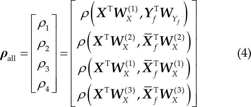
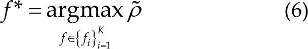
The four correlation values are combined using the following equation:

$\tilde{\rho }={\displaystyle \sum }_{i=1}^4\text{sign}\left({\rho }_i\right){\rho }_i^2$

5

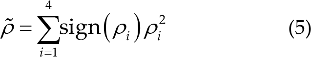
Similar to CCA, the stimulation frequency is determined by the largest $\tilde{\rho }$ :

$f^{\ast }=\underset{f\in {\left\{f_i\right\}}_{i=1}^K}{\text{argmax}}\tilde{\rho }$

6

2.4 Task task-related component analysis and ensemble task task-related component analysis

Tanaka et al. [21] proposed TRCA to process near-infrared spectroscopy data and Nakanishi et al. [14] first used it in SSVEP-based BCIs. The main idea of TRCA is to extract the task-related components by maximizing the reproducibility during the task period. When applied to SSVEP-based BCIs, TRCA maximizes reproducibility among multiple trials to improve SNR and suppress the background electrical activities.

TRCA decomposes an EEG trial x (t)∊R ^N C with N _C channels into the task-related component s (t) and task-unrelated component n (t) as follows:

$x_j\left(t\right)=a_{1,j}{s}_j\left(t\right)+a_{2,j}{n}_j\left(t\right),j=1,2,\mathrm{...},N_C$

7

where a_1,j and a_2,j are mixing coefficients. TRCA determines a weight vector w _k (k indicates the class k) to maximize the task-related component obtained by maximizing inter-trial covariance after spatial filtering as follows:

$w_k^{\text{T}}S{w}_k={\displaystyle \sum }_{\begin{array}{c}{h}_1,h_2=1\\ h_1\ne h_2\end{array}}^{N_k}{\displaystyle \sum }_{j_1,j_2=1}^{N_{\text{C}}}{w}_{k,j_1}{w}_{k,j_2}\mathrm{cov}\left[x_{j_1}^{\left(h_1\right)}(t),x_{j_2}^{\left(h_2\right)}(t)\right]$

8

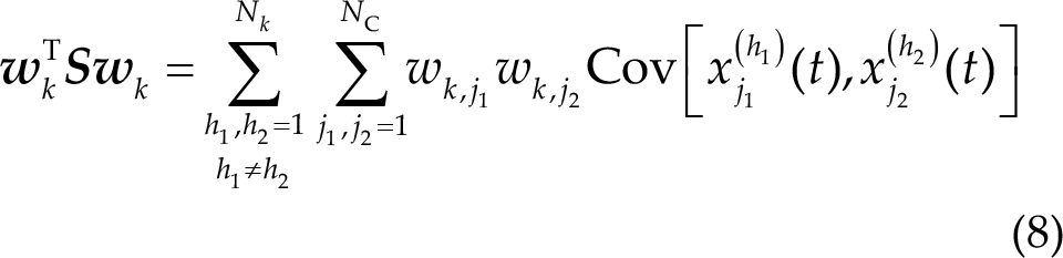
where N _k is the number of trials of class k.

A constraint of the variance of the weighted signal is added to solve the above problem as follows:

$w_k^{\text{T}}Q{w}_k={\displaystyle \sum }_{j_1,j_2=1}^{N_{\text{C}}}{w}_{k,j_1}{w}_{k,j_2}\mathrm{cov}\left[{\tilde{x}}_{j_1}(t),{\tilde{x}}_{j_2}(t)\right]=1$

9

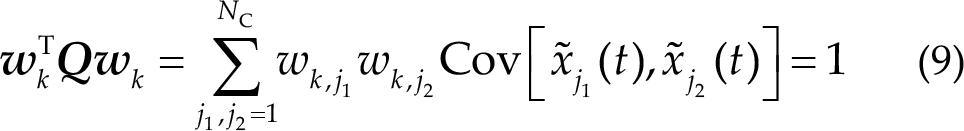
where $\tilde{x}\left(t\right)=\left[x^1\left(t\right),x^2\left(t\right),\dots ,x^{N_k}\left(t\right)\right]$ is a concatenated matrix of all training trials of class k.

Consequently, the weight vector w _k of class k can be obtained by solving the following optimization problem:

$w_k=\underset{{\widehat{w}}_k}{\text{argmax}}\frac{{\widehat{w}}_k^{\text{T}}S{\widehat{w}}_k}{{\widehat{w}}_k^{\text{T}}Q{\widehat{w}}_k}$

10

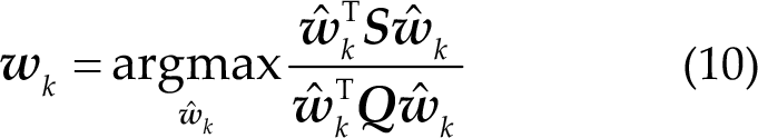
Then, the class of the trial calculated using TRCA is given as follows:

$\tau =\underset{k}{\text{argmax}}\rho \left(X^{\text{T}}{w}_k,{\overline{X}}_k^{\text{T}}{w}_k\right),k=1,2,\dots ,K$

11

Unlike TRCA, eTRCA concatenates all weight vectors to compose a common spatial filter W ∊ℝ^{N _C ×K} for all classes:

$W=\left[w_1,w_2,\dots ,w_K\right]$

12

Then, Eq. (11) can be modified as follows:

$\tau =\underset{k}{\text{argmax}}{\rho }_2\left(X^{\text{T}}W,{\overline{X}}_k^{\text{T}}W\right),k=1,2,\dots ,K$

13

where ρ2 ( X , Y ) indicates the two-dimensional correlation analysis between X and Y .

2.5 Filter bank method

Chen et al. [17] first used the filter bank method to enhance the performance of CCA, called FBCCA. Besides FBCCA, the filter bank method can be applied to all approaches, e.g., eCCA (FB_eCCA), TRCA (FB_TRCA), and eTRCA (FB_eTRCA). Filters with different passbands are applied to the original EEG trial to decompose it into several sub-band components. The i-th filter has the same upper cut-off frequency of 88 Hz with all other filters and a different lower cut-off frequency of i ×8 Hz. Consequently, a weighted summation of squares of these correlation coefficients is calculated as the feature for target classification:

${\rho }_k^{\text{fb}}={\displaystyle \sum }_{i=1}^{N_{\text{fb}}}w(i){\rho }_{k,i}^2$

14

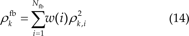
According to Ref. [17], the weight for i-th sub-band is defined as follows:

$w(i)=i^{-1.25}+0.25,i=1,2,\dots ,N_{\text{fb}}$

15

where N _fb is the number of filters.

In Algo-C, the contestants used a different weighting method based on the kurtosis of the coefficients of the same sub-band, i.e.,

$w\left(i\right)=\text{kurtosis}({[{\rho }_{{ }_{1,i}},{\rho }_{{ }_{2,i}},\mathrm{...},{\rho }_{{{ }_K}_{,i}}]}^T),i=1,2,\mathrm{...},N_{\text{fb}}$

16

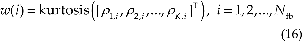
Then, they used SoftMax to normalize the weight coefficients as follows:

$w(i)=\frac{{\text{e}}^{w(i)}}{{{\displaystyle \sum }}_{i=1}^{N_{\text{fb}}}{\text{e}}^{w(i)}},i=1,2,\dots ,N_{\text{fb}}$

17

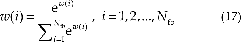
Consequently, they used this method to extend FBCCA (FBCCA_k).

2.6 Dynamic window framework

ITR (bit/min) is the most critical metric in SSVEP-based BCIs, and its calculation formula is given as follows:

$ITR=60\left[{\log }_{2}K+P{\log }_{2}P+(1-P){\log }_2\frac{1-P}{K-1}\right]/T$

18

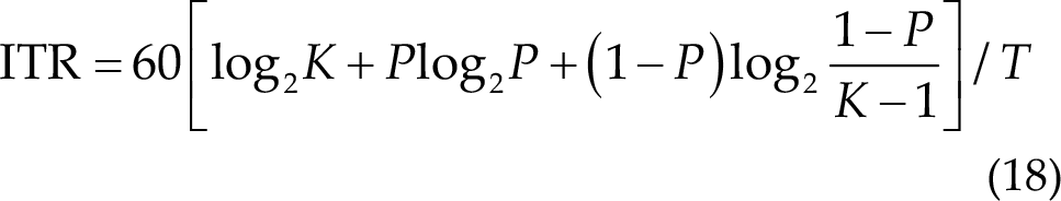
where P is the classification accuracy, and T (in seconds) is the average computing time (replacing with test data length in the final). ITR was ideally calculated, meaning that the gaze shifting time was not included in the ITR calculation. Thus, to obtain a high ITR, the data length should be short. Obviously, the shorter the data length, the lower the classification accuracy. Therefore, it must obtain a balance between the data length and accuracy.

The optimal data length is distinctive and susceptible from trial to trial due to spontaneous EEG’s complexity and nonstationarity [22]. Thus, using a fixed data length for all trials is inappropriate. The dynamic window framework [22, 23] is suitable under this circumstance. As it was an online environment and data were provided in the form of data packets, the algorithm could calculate the result after getting sufficient data and choose to continue to get data if the result’s confidence was not sufficiently high. Its main idea is to set a standard to judge whether the current result meets the requirement. If not, the algorithm will continue to get data until the requirement is satisfied. Usually, the algorithm needs to set a minimum length, maximum length, and interval.

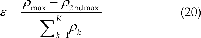
There were mainly two dynamic window strategies used in the final. The first strategy tries to compute a confidence score from the correlation coefficients of all classes and set a threshold used by all teams. If the score exceeds the threshold, the result is credible, and the algorithm stops receiving data and outputs the results. The teams used three methods to obtain the confidence score. One was based on the risk function proposed in [22], which could be computed as follows:

$\epsilon =\frac{-\left({\rho }_{\max }-{\rho }_{2\text{ ndmax }}\right)}{-\left[{{\displaystyle \sum }}_{k=1}^K{\rho }_k-K\log \left({{\displaystyle \sum }}_{k=1}^K{\text{e}}^{{\rho }_k}\right)\right]}$

19

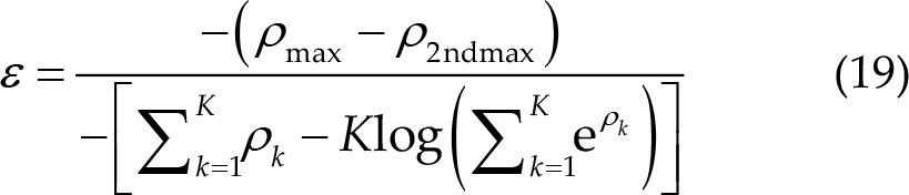
It was also used in Algo-H, Algo-M, and Algo-C. Under this circumstance, the score ε needs to be smaller than the threshold th to indicate that the result is credible. Algo-L used another score computing method, given by

$\epsilon =\frac{{\rho }_{\max }-{\rho }_{2\text{ndmax }}}{{{\displaystyle \sum }}_{k=1}^K{\rho }_k}$

20

The contestants used the kurtosis of the correlation coefficients as the score in Algo-B. In Algo-L and Algo-B, the score ε needs to be greater than the threshold th to prove the result’s credibility. The threshold th was determined through cross-validation using preliminary data.

Besides the above strategy, in Algo-H, we used a strategy based on integrating different algorithms. We used four algorithms (CCA, FBCCA, eCCA, and eTRCA) and determined whether to output the result according to the voting results of the algorithms. The result is credible when half of the algorithms gives the same results. We used the following rules in the final:

$\text{If}\hspace{0.17em}{L}_{\text{eTRCA}}==L_{\text{eCCA}}\hspace{0.17em}\text{and }(L_{\text{eTRCA}}==L_{\text{CCA}}\text{or}\hspace{0.17em}{L}_{\text{eTRCA}}==L_{\text{FBCCA}}),\text{ then output the result}$

21

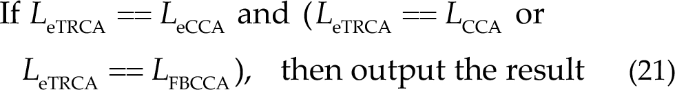
where L denotes the label given by the algorithms.

2.7 Training strategy in calibration-free scenario

Although the contestants had no access to training data from the subjects in the final, they could use data from the subjects in the preliminary. In Algo-L, the contestants used data from the preliminary to train the filters and templates of TRCA. Similarly, the contestants used data from the preliminary to train the filters of TRCA in Algo-M; however, they used sine–cosine reference signals as templates. In Algo-H, we trained TRCA and eCCA models in the same way.

However, it is not easy for the models trained on old subjects to perform well on the new subjects. In Algo-H, we tried using the first block data to update the models to solve this problem. When a test trial came, we used the results of CCA and FBCCA as the label. Then, we used the trial to update the filter and template of eTRCA and eCCA of the corresponding class. To ensure the accuracy of the label, we set a sufficiently long data length (2 s, longer than the maximum length used in the dynamic window framework) for the first block data. Furthermore, we used dynamic updating and dynamic window frameworks simultaneously, where we updated the models when the results were credible.

2.8 Flowcharts of five teams

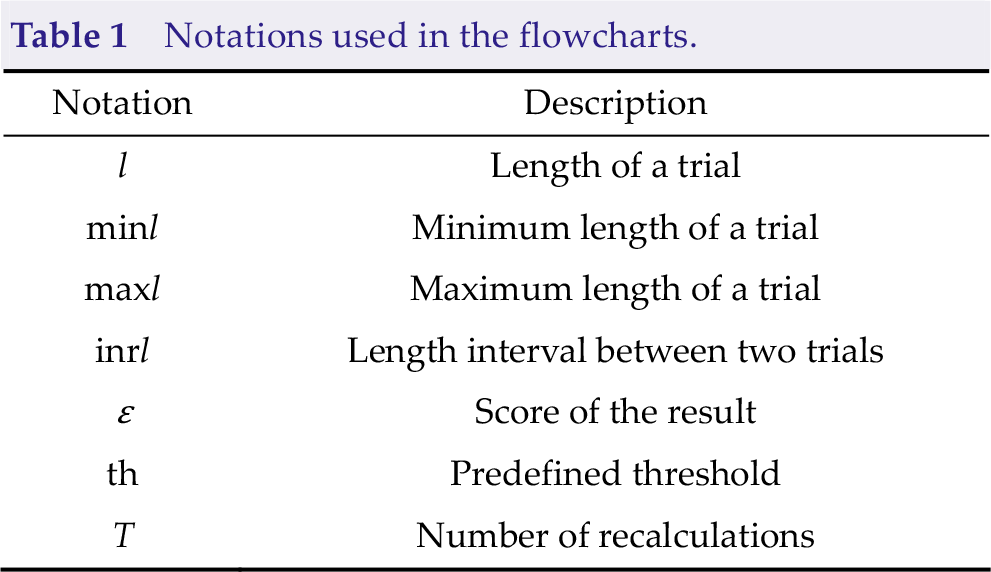
Figure 3 shows the flowcharts of the five algorithms. Table 1 presents notations used in the flowcharts. Algo-H uses the current user’s data to update the models; thus, it is time-consuming. The frameworks of the other four algorithms are similar, meaning that their computational cost is also similar.

Fig. 3

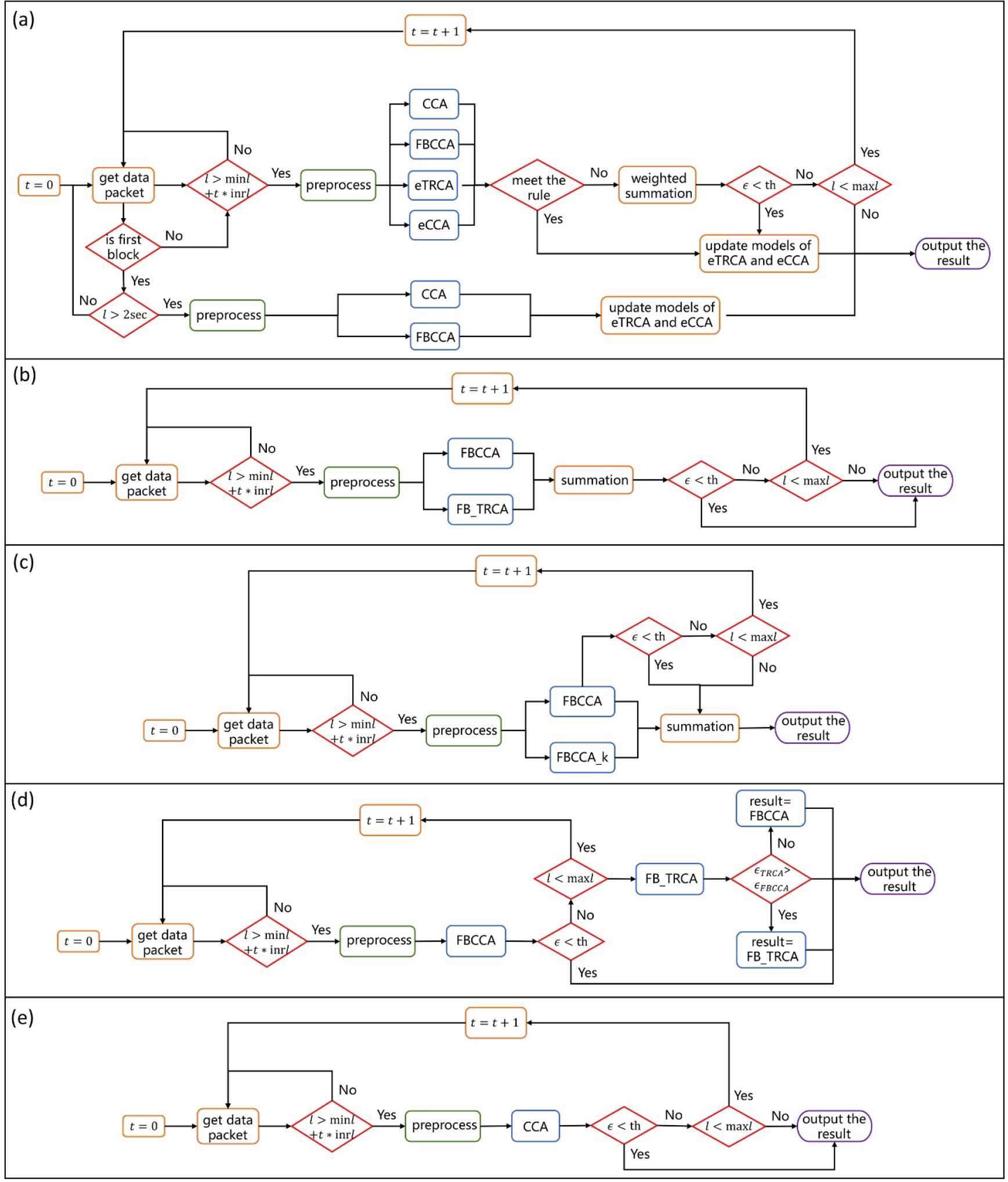
Flowcharts of the five algorithms. (a) Algo-H. (b) Algo-M. (c) Algo-C. (d) Algo-L. (e) Algo-B.

Table 1

Notations used in the flowcharts.

Notation	Description
l	Length of a trial
minl	Minimum length of a trial
maxl	Maximum length of a trial
inrl	Length interval between two trials
ε	Score of the result
th	Predefined threshold
T	Number of recalculations

3 Results

3.1 Experiment results in the final

The competition was approved by the institutional review board of Tsinghua University (NO. 20210032). The competition was in the calibration-free scenario, meaning that the subjects were the first time to use the system, and the contestants had no access to the subjects’ training data. This scenario is slightly different from the traditional calibration-free approaches, where the contestants can use calibration-free approaches and use models trained with other subjects’ data. EEG data were recorded using a 64-channel wireless EEG acquisition system (Neuracle China) with a sample rate of 1000 Hz. The raw data were down-sampled to 250 Hz. The frequency of the power line noise was 50 Hz. The contestants could only use the eight channels near the optical area (POz, PO3, PO4, PO5, PO6, Oz, O1, and O2). The graphical user interface (GUI) presented a cue for 1 s to make subjects focus on the highlighted target during each trial. Then, all target characters flickered for 4 s. After stimuli, the result was calculated using calibration-free algorithms and highlighted on the GUI as feedback for 1 s. During the test, the system provided data in an online environment. Whenever calling the getData function, the system would provide a new data packet, including EEG data, and trigger information with a data length of 120 ms. In the same block, data packets were in order. If the test data included multiple blocks and data of the current block were all sent out, EEG data of the new block would be sent when calling the getData function next time. Each subject had three blocks of data in the final. The system was fully online; thus, the algorithms must calculate the result within 4 s.

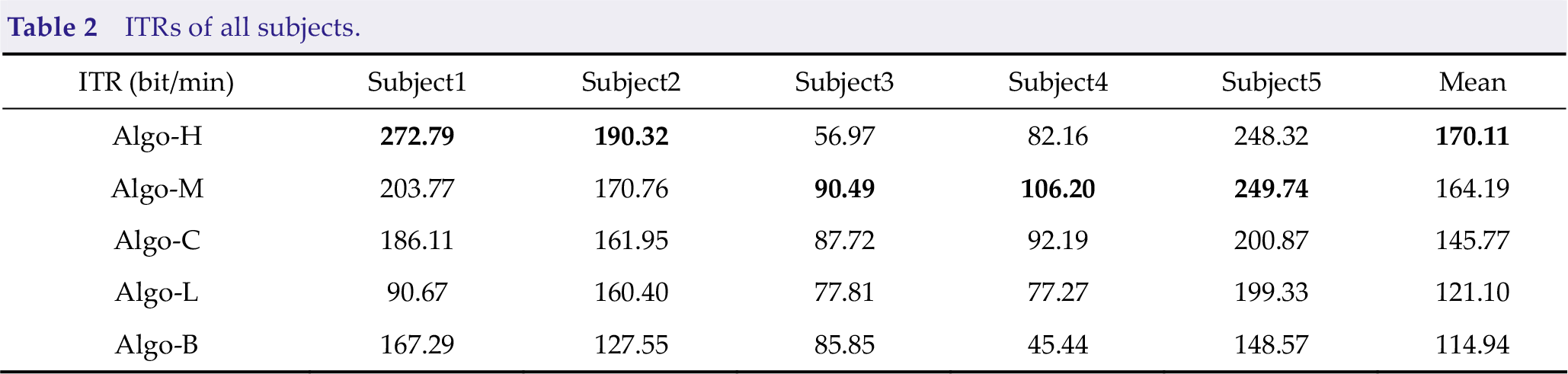
There were five subjects in the final, and each subject had three blocks of data. All five subjects were male and aged 20–25 years. Table 2 presents the mean ITRs of the five subjects. Different subjects had different results because of differences in environment and subject proficiency. The ITRs of Subject1, Subject2, and Subject5 were much higher than those of Subject3 and Subject4. Algo-H and Algo-M performed much better than other algorithms. Of the two algorithms, Algo-H had an outstanding performance on skilled subjects, whereas Algo-M had good performance on all subjects. In other words, the performance of Algo-M is more stable, and Algo-H is more suitable for skilled subjects. Algo-M’s performance on all subjects is better than all other algorithms, except Algo-H, meaning that FB_TRCA is suitable for the scene.

Table 2

ITRs of all subjects.

ITR (bit/min)	Subject1	Subject2	Subject3	Subject4	Subject5	Mean
Algo-H	272.79	190.32	56.97	82.16	248.32	170.11
Algo-M	203.77	170.76	90.49	106.20	249.74	164.19
Algo-C	186.11	161.95	87.72	92.19	200.87	145.77
Algo-L	90.67	160.40	77.81	77.27	199.33	121.10
Algo-B	167.29	127.55	85.85	45.44	148.57	114.94

The ITRs of all blocks are shown in Fig 4. In Algo-H, we used a long data length for the first block; thus, the ITRs of the first block of all subjects are lower than other algorithms. On Subject1, Subject2, and Subject5, the ITRs of the second and third blocks improved significantly, proving that using the first block to update the models is very effective. However, on Subject2 and Subject3, the ITR of the second block is lower than that of the first block. Therefore, when the data quality is poor, and the accuracy of the pseudo-labels cannot be guaranteed, it is inappropriate to update the models with the first block data.

Fig. 4

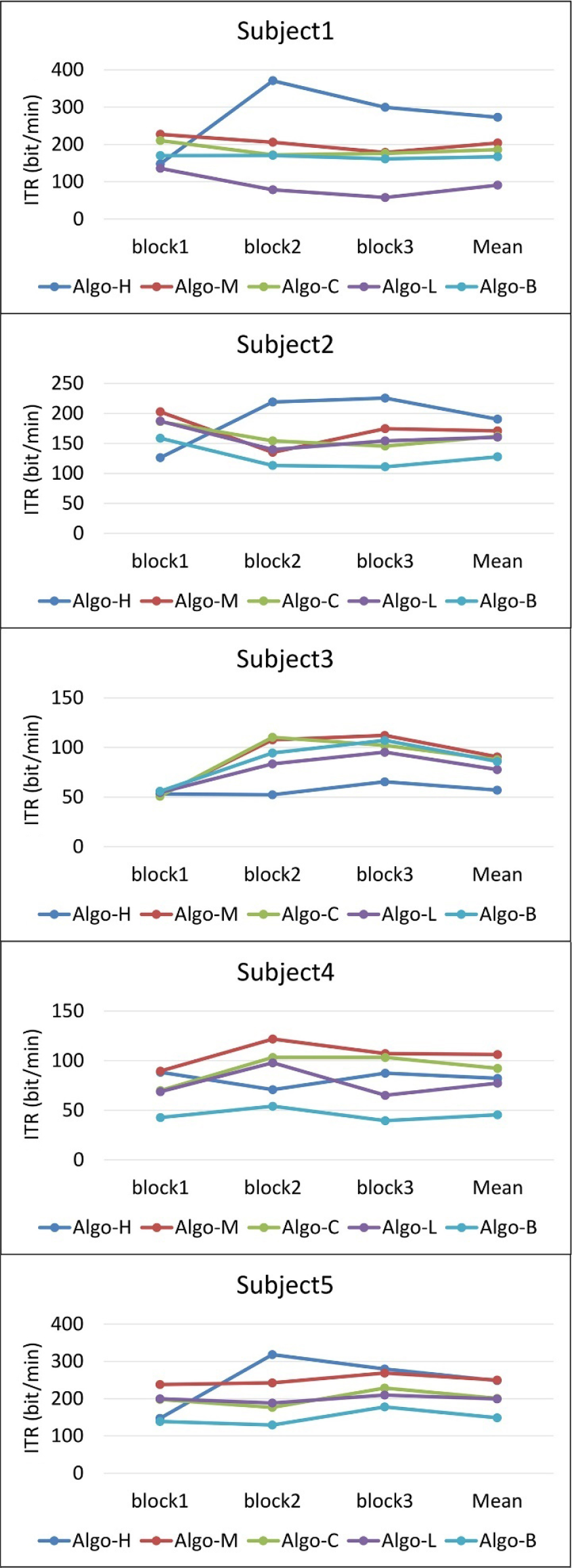
ITRs of all blocks.

3.2 Offline experiment results

We tested the performance of the algorithms on the benchmark dataset. The benchmark SSVEP dataset was first introduced by Wang et al. [24] in 2017. The visual keyboard of the speller used in the benchmark dataset was the same as that used in the competition. Thus, the benchmark dataset can be directly used in this study. There were 35 subjects and six blocks of EEG signals were collected from each subject. In each block, there were 40 trials corresponding to all 40 targets.

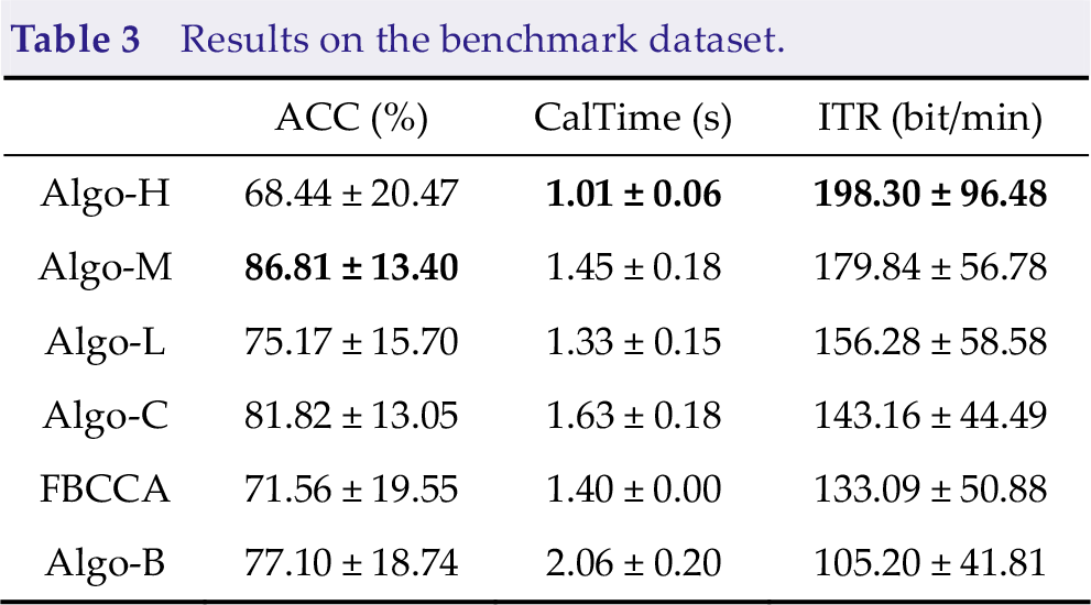
Table 3 presents the average accuracy (ACC), average calculating time (CalTime), and average ITR of the algorithms on the benchmark dataset for all subjects. In addition to the above five algorithms, we added FBCCA as a comparison. For FBCCA, the calculating time was fixed at 1.4 s. All algorithms performed better than FBCCA, except Algo-B, proving the effectiveness of the dynamic window framework. Algo-H had the shortest calculating time; therefore, it had the highest ITR, even with lower accuracy. The standard deviation of the ITR of Algo-H was the largest, meaning that Algo-H varied greatly among different subjects. Figure 5 shows that Algo-H performed much better than other algorithms on many subjects. Algo-H performed poorly only on very few poor subjects.

Table 3

Results on the benchmark dataset.

	ACC (%)	CalTime (s)	ITR (bit/min)
Algo-H	68.44 ± 20.47	1.01 ± 0.06	198.30 ± 96.48
Algo-M	86.81 ± 13.40	1.45 ± 0.18	179.84 ± 56.78
Algo-L	75.17 ± 15.70	1.33 ± 0.15	156.28 ± 58.58
Algo-C	81.82 ± 13.05	1.63 ± 0.18	143.16 ± 44.49
FBCCA	71.56 ± 19.55	1.40 ± 0.00	133.09 ± 50.88
Algo-B	77.10 ± 18.74	2.06 ± 0.20	105.20 ± 41.81

Fig. 5

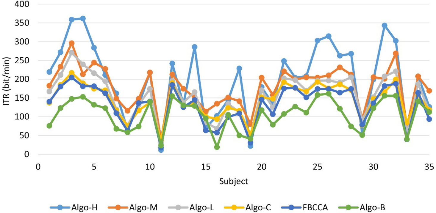
ITRs of all subjects from the benchmark dataset.

Figure 6 shows the average ITRs of all subjects on different blocks. Similar to the results in the final, the ITR of the first block of Algo-H was much lower than other algorithms, except Algo-B. However, the ITRs of the remaining blocks of Algo-H were much higher than all other algorithms. Consistent with the above conclusion, the standard deviation of the ITR of Algo-H was the largest. Thus, not all subjects were suitable for the strategies used by Algo-H.

Fig. 6

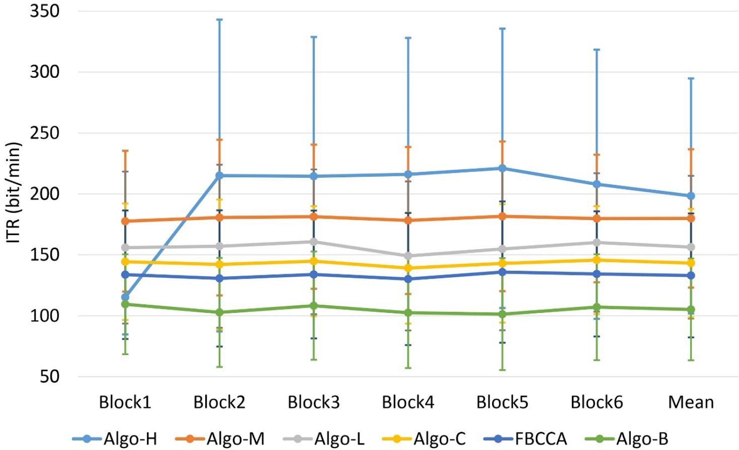
ITRs of all blocks from the benchmark dataset.

4 Discussion

This paper introduces the algorithms used by the top five teams in the final of the SSVEP competition (calibration-free) of the WRC2021. The algorithms used several new approaches to improve the performance of SSVEP in calibration-free scenarios.

By comparing the ITRs of the first and following blocks, we can prove that using the first block of data to update models is helpful. However, it may lower the ITR on the first block because it needs a long data length to guarantee the accuracy of the pseudo-labels. Furthermore, the quality of data for unskilled subjects is poor. Therefore, updating models under this circumstance may degrade performance. Thus, in a real-world calibration-free system, the system can use the data from the initial stage to update the models when the subject is not entirely unskilled. The system can adjust data length at this stage according to data quality.

In the preliminary stage, we obtained that the performance of the dynamic window framework based on the integration of different algorithms was much better than the traditional dynamic window framework when the data quality is not that good. Because when the data quality is outstanding, TRCA or eCCA may perform well with a pretty short data length, whereas CCA and FBCCA may perform poorly, making the integration inoperative. The results on the benchmark dataset proved that our dynamic window framework is suitable for most subjects. Consequently, integrating different algorithms instead of using only one algorithm effectively improves performance in a real-world system. So almost all teams used this strategy.

5 Conclusion

In this paper, we introduce algorithms used by the top five teams, Algo-H, Algo-M, Algo-C, Algo-L, and Algo-B, in the final of the SSVEP competition (calibration-free) of the WRC2021. These algorithms provide some new ideas for dealing with SSVEP calibration-free scenarios. Some ideas may be helpful for real-world systems, such as updating the models with previous data and dynamic window framework based on the integration of different algorithms. In future work, we will propose a more comprehensive and practical calibration-free algorithm framework to improve the performance of SSVEP in the calibration-free scenario.