Sage Journals: Discover world-class research

Abstract

Textile defect detection and classification is an important part of the textile production process, however, to detect accurately and efficiently is still difficult. In this study, we present an effective formulation for textile defect detection. Unlike traditional textile detecting methods, a conventional neural network (CNN) support vector machine (SVM) is designed to extract the depth features of textile images and to classify defects. The effectiveness of textile feature extraction is improved by optimizing Alexnet to obtain a CNN with better feature extraction and less computation. Textile defect classification is more effective using SVM instead of Softmax. Experimental results demonstrated that the improved Alexnet-SVM gave 99% accuracy in defect classification using the TILDA database. This accuracy was 5% greater than Alexnet and GoogleNet.

Keywords

Computer Vision Convolutional Neural Network Improved Alexnet SVM Textile Defect Classification Textile Defect Detection

Introduction

Defects of textiles have the characteristics of multi-scale, various cloth types, and complicated background texture, which brings difficulties for the entire textile inspection process. Therefore, detecting textile defects has important scientific research value. There are four main defect detection algorithms: statistical,^1,2 frequency spectrum,^3,4 model,^5,6 and pattern methods.⁷ Among these four methods, the frequency spectrum method is popular in textile defects detection since it is stable in feature extraction. The frequency spectrum method has the following methods in practical application: Fourier transform method,⁸ Gabor filter method,⁹ wavelet transform,¹⁰ and filtering approach.^11,12 An optimized Gabor filter was proposed to set up a defect detection model based on the analysis of fabric defect characteristics. The composite differential evolution is used to optimize the Gabor filter parameters and achieve an optimal feature extraction of fabric defects.¹³ However, this method is not effective to extract the discrimination between the defect and the background.

On one hand, all the methods mentioned above are traditional defect detection methods. Their detection process is complex, and the accuracy of detection cannot meet the requirements of industrial production. On the other hand, convolutional neural networks (CNN) have made great progress in defect detection. In one study, a novel cascaded auto encoder (CASAE) architecture and CNN was designed to automatically detect defects on metal surfaces.¹⁴ The experimental results show that the method meets the requirements for robustness and accuracy of metal defect detection. In one study,¹⁵ a multi-step CNN was proposed to classify defects on the inner surface of tires, and the accuracy was improved by 17%. A multi-class defect detection model for electrical equipment was proposed in another study based on a fast region-based R-CNN model.¹⁶ This model is more effective and accurate than traditional detection methods. It is precisely because of the excellent performance of CNN in the field of computer vision that we propose a method for classifying textile defects based on CNN models.

Softmax is a common collocation classifier for CNN, but we found in some literature that CNN is better with a support vector machine (SVM). A method was proposed for identifying brain tumors based on the CNN-SVM model, and achieved excellent results.¹⁷ Other researchers proposed a CNN-SVM model for gesture recognition.¹⁸ Experimental results show that the model is more promising and efficient than existing methods such as hue saturation value + random decision forest (HSF + RDF), scale-invariant feature transform + partial least squares (SIFT + PLS), model predict control (MPC), and classic CNN. Therefore, we propose a CNN-SVM model to be compared with the CNN model and some previously proposed textile classification models. The results show that CNN-SVM performed better for classification accuracy.

The main contributions of this study are threefold: 1) To extract deep features for defect detection and classification based on Alexnet. By using Alexnet, the classification accuracy of the verification set can reach 94% using the TILDA dataset.¹⁹ 2) To propose an improved algorithm based on Alexnet, which has an accuracy of 95% in the verification set. 3) Since Softmax is not the optimal solution for classification algorithms, a method for classifying textile features extracted by improved Alexnet is proposed by developing an SVM classifier; the accuracy of this method in the validation set reached 99%. In short, this study presents an improved Alexnet that can extract more effective features, and designs a SVM classifier to improve the accuracy of classification.

The content of this paper is organized as follows. The basic theories are described. The CNN framework and SVM classifier designed in this paper are then described. The data and parameters of the training are described next, followed by the conclusion.

CNN and Classifier

CNN

CNNs are widely used in the field of computer vision. It mainly contains six layers as follows.

Convolution Layer

The convolution operation is the summation of two variables after they are multiplied. Convolution enhances the input signal and reduces the noise. The smaller the convolution kernel, the finer the processing of the image, but it also means that more convolutional layers are needed to conduct feature extraction.

Activation Function

The activation function is used to increase the fitting ability of the network. It is usually used between the nodes of the neural network. Krizhevsky et al. proposed the Relu activation function to solve the problem of gradient disappearance and reduce large computational complexity²⁰ Eq. 1 is the formula for the Relu function. Use of the Relu activation function can reduce the amount of computation, however, the activation function can increase the sparsity of the network and solve the overfitting problem.

f_{k s} (x) = \max (x, 0)

(Eq.1)

Pooling Layer

After the convolution operation, a large quantity of image redundancy still exists. To handle this problem, the image should be down-sampled. This is called “pooling,” which is the most important role to prevent the network from overfitting.

Fully Connected Layer

The main function of the fully connected layer is to integrate the feature map of the previous layer and output features which contain higher level semantic content. Usually the output of this layer indicates the class categories for the classification purpose.

Local Response Normalization (LRN)

Krizhevsky et al.²⁰ first proposed the LRN layer to introduce a competitive mechanism for local neurons, which leads to a larger probability value of the neuron response, and inhibits other neurons with less feedback so as to enhance the generalization ability of the model.

Dropout

Dropout randomly discards some neurons during training. Neurons that have undergone this operation are not involved in the spread. Thus every training will produce a different network structure. This method can effectively reduce the amount of calculation and reduce the possibility of overfitting.

Classifiers

Softmax

When CNN is used for multi-classification, the Softmax classifier is usually used. The classifier converts the output value of the network into the probability of each category, and the category with the highest probability is the prediction category. The Softmax value is calculated as in Eq. 2.

S_{i} = e^{(T_{i})} / (\sum_{j} e^{(T_{j})})

(Eq.2)

T is any array, and i and j represent the subscript values of an element of the array T, respectively.

Loss is defined as cross entropy and represented by Eq. 3.

L_{i} = - \log (e^{(T_{i})} / (\sum_{j} e^{(T_{j})}))

(Eq.3)

Softmax encourages the output of real target categories to be larger than other categories, but the value of such an output cannot be too large, so this classification output more easily creates errors than SVM.

SVM

The ultimate goal of SVM is to find an optimal linearly separable hyperplane to distinguish different categories. The optimal linear separable planes divide different data with the greatest distances to obtain different categories. Let the classification set be S = {(x_i,y_i)|I = 1,...,n}, where x_i∈Rd, y_i = {+1,–1} is the category label corresponding to x_i. Let the classification plane function be f(x) = w^Tx+b, where w is the weight and b is the offset. If the above function is converted into an equation, then the equation is w^Tx+b = 0.

After normalizing f(x), when |f(x)|≥1 is satisfied for S, the classification interval is 2/(‖w‖). Therefore, the problem of achieving the ultimate goal of SVM can be translated into the weight optimization problem to satisfy the condition given in Eq. 4.

y_{i} [(w^{T} x) + b] - 1 \geq 0, i = 1, 2, \dots, n

(Eq.4)

Eq. 4 aims to ensure that the divided defect get the correct results. The solutions to extend the classifier to a multi-classifier are one-against-one, one-against-all, direct modification of classification formulas, and so on.

Model Implementation

Alexnet

When Alexnet was introduced, CNN began to be widely used in the field of computer vision. Alexnet's input is 256*256*3, where the width and height of the image are 256, and the color channel is 3. Alexnet is randomly cropped into 227*227*3 images at the data layer, which is also a way of data enhancement (Fig. 2).

Fig. 1

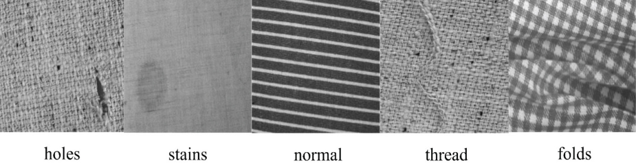
Five classes of defect images.

Fig. 2

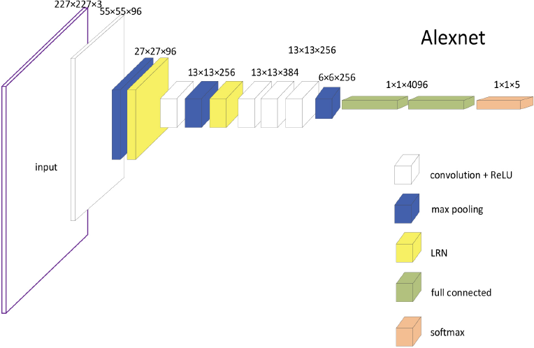
Alexnet schematic.

In the first layer, the number of convolution kernels is the output data dimension (namely 96 in this work), the convolution kernel size is 11*11, and the step size is 4. After the convolution layer, the size of the image becomes 55*55*96; after the function layer is activated by Relu, the size of the image does not change. Then through the pooling layer, the pooling strategy is max-pooling, the kernel size is 3, the stride is 2, and the output data size is 27*27*96. Finally, there is a normalization layer, which is a local normalization layer (LRN) with a local size of 5, a scaling factor (alpha) of 0.0001, and an exponent term (beta) of 0.75. The norm layer does not change the size of the data.

In the second layer, the operations performed are basically the same as the first layer. However, the number of convolution kernels is 256, the size of the convolution kernel is 5*5, and the step size is 1. Unlike the first layer, the convolution layer strategy keeps the data size unchanged after the convolution (same strategy) and adopts the padding operation by setting the padding edge to a value of 2. The pooling layer and the normalization layer calculation (norm layer) strategy are consistent, so the output of the second layer is 13*13*256.

The third and fourth layers have no normalization layer and pooling layer. With the image size invariant strategy after operation, the number of convolutional layers is 384, the convolution kernel size is 3, and the padding edge is 1. The resulting data size is 13*13*384.

The fifth layer is calculated in a similar manner to the first layer and the second layer. The number of convolution kernels is 256, the convolution kernel size is 3, and the padding is 1. The output of the convolutional layer is 13*13*256. However, there is no local normalization operation for this layer, that is to say, no norm layer exists. The resulting data size is 6*6*256, which converts the data into a long vector output of length 9216.

The sixth to eighth layers are fully connected layers, which are different from the previous layers, and the layers do not share weights. The number of cores for the sixth and seventh layers is 4096. Both the sixth and seventh layers have adopted the Dropout strategy, and the value of Dropout is set to 0.5. The core of the eighth layer is 1000 nodes, and it can be classified into 1000 classes by inputting it into the Softmax regression function layer. The classification performed in this paper is Category 5, so the 1000 outputs are changed to 5 outputs to complete the classification of textile image defects. However, Alexnet has three shortcomings that cannot be ignored. 1) Alexnet's numbers of parameter are too large for the small sample used in this study. 2) Alexnet's first layer of convolution kernels is too large to extract finer features, which is detrimental to feature extraction of textile images with very small defects. 3) Constrained by the hardware capabilities of the era proposed by Alexnet, Alexnet uses group convolution. However, a fatal disadvantage of group convolution is that information flow is reduced between channels of different groups, that is, the output feature maps only consider part of the input features.

Improved Alexnet

Improved Alexnet is designed based on VGG-Net²¹ and it has deeper and thinner network when comparing with Alexnet. VGG-Net has three main advantages: 1) The first layer has a small quantity of filters and short steps. 2) The training model is adaptive to multi-scale changes. In addition, VGG-Net uses a 3*3 convolution kernel with a step size of 1 and a pixel. 3) The LRN layer has no influence on the feature extraction of textile images, and has no obvious improvement effect (Fig. 3).²¹

Fig. 3

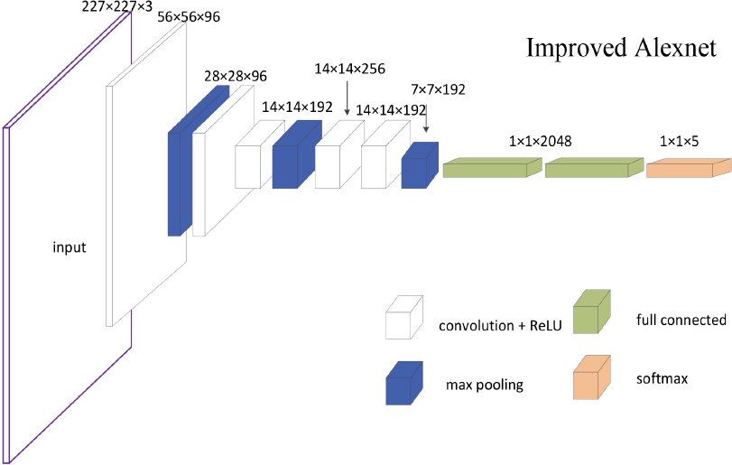
Improved Alexnet schematic, which was thinner and less computation than Alexnet.

According to VGG-Net, the small size of convolution kernels normally has implicit rules, which can capture finer features; and two 3*3 convolution kernels can replace 5*5 convolution kernels, making the network more nonlinear with fewer number of parameters. Therefore, this study proposes to replace Alexnet's 11*11 convolutional layer with a 9*9 convolutional layer, and replace the second layer of 5*5 convolutional layer with two 3*3 convolutional layers using the same strategy. This layer reduces the number of convolution kernels to 192. In addition, according to the experimental results of VGG, the effect of the LRN layer is small and the amount of calculation is increased, so this section deletes the LRN layer of Alexnet. Finally, the number of nodes of the first and second fully connected layers is reduced from 4096 to 2048.

In general, by improving the chunky network into a thin and deep network, the depth of the network is increased while reducing the number of parameters, so that the improved network does not sacrifice any performance or even has better performance. The data set used in the Alexnet had an image size of 256*256*3, but when the image was entered into the input layer, the image size of improved Alexnet was randomly cropped into 227*227*3. At the first level, after passing through the convolutional layer, the size of the image becomes 56*56*96; the function layer is then activated by Relu. After the pooling layer, the pooling strategy is the maximum pooling, kernel size is 3, stride is 2, and the output data size is 28*28*96; this section uses a consistent pooling layer. In the second layer, the convolution layer fill edge is 2. The second layer has no pooling layer, so the output of the second layer is 28*28*96. The second and third layer calculation strategies are the same. But the third layer has a pooling layer, and the output data size is 14*14*192.

The strategy of the fourth and fifth layers is the same. Only the filter layer and the Relu function, the output of the convolutional layer is 14*14*256. The output of the sixth layer of the convolutional layer is 14*14*192. The sixth layer has a pooling layer, and the resulting data size is 7*7*192, which converts the data into a long vector output of 9408. The seventh to ninth layers are fully-connected layers, and the sixth and seventh layers have a core number of 2048. Both the seventh and eighth layers have adopted the Dropout strategy, and the value of Dropout is set to 0.5. The eighth-layer kernel number is 5, and it can be classified into five categories by inputting it into the Softmax regression function layer.

Multi-Class SVM

To improve the accuracy of classification, this section uses SVM instead of Softmax. The method is based on Hinge-Loss.²² The multi-class SVM based on HingeLoss is more like a “real” multi-class SVM (Eq. 5).²³

1 (y) = \max (0, 1 +_{t \neq y}^{\max w_{t} x} - w_{y} x)

(Eq.5)

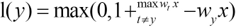
If the score of the correct label exceeds the score of the other label by at least 1, the loss value is 0. Otherwise, the loss value is the correct label score that is at least 1 point lower than the other label scores. In the case of a small number of data sets, Eq. 5 provides a suitable method to improve the classification accuracy. It essentially distinguishes between statistical methods and does not require a large amount of data to improve classification accuracy. And its implementation process is simple and straightforward, which simplifies the difficulty of implementation.

Experiments

Experimental Data

This study used the TILDA image library to conduct the experiments. As shown in Fig. 1, this work examines and classifies the five types of textile images (numbered 0, 1, 2, 3, 4) for holes, stains, normal, thread, and folds.

There are more than 300 images of each defect, and the image is expanded by 4 times by rotating the image 90° and 180°, Gaussian noise, and changing the image color difference, for a total of 8105 sheets. Among them, 1653 were broken, 1390 were stains, 1456 were normal, 1646 were threaded (knotted), and 1960 were folded. Among them, the training set (6484) and the verification set (1621) were randomly divided into 8:2 ratios, and a test set (20 in each category) was set up, which did not participate in training and verification. The image library used in this study is a grayscale image, so the image is unified into a 256*256*3 color image.

Training

The experiments in this work are based on the cafe²⁴ framework and the GeForce GTX 1080Ti. The training of CNN belonged to supervised training. The input training data was marked with the correct category and learned various network parameters. Verification was the use of the network at the time of verification, predicting the type of image of the validation set and comparing it to the correct category label. The calculation formula for the accuracy of the verification set is given in Eq. 6.

a c c = (\frac{V_{r i g h t}}{V_{t o t a l}}) * 100 %

(Eq.6)

acc is the classification accuracy, V_right is the right classification, and V_total is all the samples. The training process of convolutional neural networks is as follows. 1) The Gaussian distribution was used to randomly initialize the parameters of each layer W. With such a setting, the initial value of the parameter can be made smaller, and saturation did not occur. The Gaussian distribution had a mean of 0 and a variance of 0.01. The parameter b was set to a constant of 0.1. 2) Took 150 training data in turn to participate in the training. 3) Calculated the corresponding output y according to the current network parameters and the label corresponding to the image to calculate the Softmax loss value. 4) Updated W and b using the gradient descent method until the training stopped.

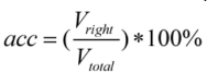
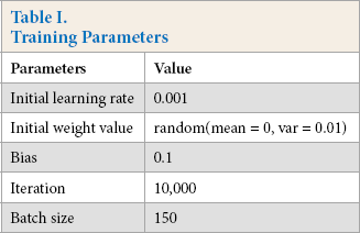
In this study, the initial learning rate α was set to 0.001, the total number of iterations was 10,000, and 150 iterations were taken for each epoch (Table I). The learning rate was reduced by 10 times every 5000 times. Verification of the verification set was performed every 1000 times, and each verification basically verified the picture of the verification set once, and the corresponding loss and accuracy were obtained.

Table I

Training Parameters

Parameters	Value
Initial learning rate	0.001
Initial weight value	random(mean = 0, var = 0.01)
Bias	0.1
Iteration	10,000
Batch size	150

Results and Comparison with Previous Work

To confirm the rigor of the experiment, this work trained and tested all three networks mentioned above. Fig. 4 is a visualization of the training and verification process for each network and the prediction of the same test picture (Class 2). This picture is a flawless picture (the flaws in the images are difficult to classify), which is the most difficult type of picture to identify for a model. Based on the left side of Fig. 4, the visualization of the training process for the models Alexnet, Improved Alexnet, and Improved Alexnet SVM (top to bottom), respectively, is shown. After 6000 iterations, the accuracy of Alexnet reached 94% and Improved Alexnet reached 95%, while Improved Alexnet SVM only needed 2000 iterations to achieve 95% accuracy, up to 99%. All three models can accurately output the classification results. Alexnet outputted class 2 with 91.34%, Improved Alexnet outputted class 2 with 99.59%, and Improved Alexnet SVM outputted class 2 with 100.00%. According to the effect of model training and testing ability, the Improved Alexnet SVM model had a stronger learning ability and more accurate classification ability. From the prediction results of Table II and Fig. 4, the prediction of SVM was the most accurate. Because of the predicted output of the SVM multi-classifier, only the correct category was positive and the other was negative, reflecting the characteristics of the maximum inter-class distance.

Fig. 4

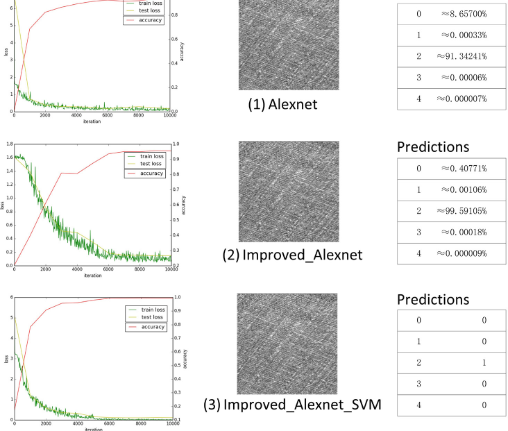
Training and verification process for each network with the prediction results of the test pictured.

Table II

Comparison of the Accuracy of the Proposed Method in Verification with Previous Research in the TILDA Dataset¹⁹

Model	Accuracy(%)
PCA + FFN²⁶	97.35
MLP neural networks²⁷	89.48
Sparse coding²⁸	93
GoogleNet	94
LeNet-5²⁹	93.81
VGG16²⁹	96.38
Alexnet	94
Improved Alexnet	95
Improved Alexnet SVM	99

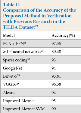
This study also trained GoogleNet²⁵ for comparison and the three other previous classification models as well. Table II provides a summary of the comparison. One study proposed a method using the feed-forward neural network (FFN) classifier to classify different features extracted from discrete cosine transform (DCT) transformed images and reported the average classification accuracy (CA) result of 97.35%.²⁶ Tabassian et al.²⁷ proposed a new approach, which was based on accepting uncertainty in labels of the learning rate and combined with the Dempster-Shafer theory of evidence, with a detection accuracy of 89.48%. Zhu et al.²⁸ proposed an algorithm based on Gabor filter and sparse coding training, which can achieve 93% accuracy in the defect detection of twill, plain, gingham, and striped fabrics. This study used the same data set (TILDA19) to train on GoogleNet and got a detection accuracy of 94%. Another study trained LeNEt-5 and VGGNet and achieved 93.91% and 96.38% accuracy on the TILDA dataset, respectively.²⁹ Although VGGNet had a higher accuracy in the TILDA dataset than Improved Alexnet, the network structure of Improved Alexnet was shallower and less computationally intensive.

Conclusions

Automated inspection of textile defects is critical to the textile industry. Unlike traditional machine learning methods, convolutional neural networks (CNNs) are extremely effective in extracting depth features of images. Based on the complexity of textile texture background and the outstanding development of CNN in defect detection, this study proposes to use convolutional neural network to extract the depth features of textile images and classify textile images according to these features. The experimental results also show that the SVM classifier was better than Softmax.

However, this work only proposes a defect classification algorithm that cannot detect the size of the defect. In fact, many small defects should be ignored in actual production, so the network itself should be able to distinguish between small defects and defects to improve actual production efficiency. In future work, we will focus on designing algorithms that ignore defects of a certain size.

Footnotes

Acknowledgements

This work was supported by the National Natural Science Foundation of China (No. 61703169) and the China Scholarship Council (CSC).

References

Alper Selver

; Avşar

; Özdemir

J. Text. Inst. 2014, 105 (9), 998–1007.

Kuo

C.-F. J.

; Su

T.-L.

; Chang

C.-D.

; Lee

C.-H.

Fiber. Polym. 2008, 9 (6), 768–775.

Ralló

; Millán

M.S.

; Escofet

Appl. Opt. 2007, 46 (27), 6688–6699.

Millán

M.S.

; Escofet

; Ralló

Unsupervised Flaw Segmentation in Textile Materials under Visible and NIR Illumination. In Optics, Photonics, and Digital Technologies for Multimedia Applications; International Society for Optics and Photonics: 77230Q, 2010.

Ozdemir

; Ercil

Proceedings, 1996 IEEE Conference on Emerging Technologies and Factory Automation. ETFA ‘96; IEEE, 1996, 2, 697–703.

Chan

H.-Y.

; Raju

; Sari-Sarraf

; Hequet

E.F.

A General Approach to Defect Detection in Textured Materials Using a Wavelet Domain Model and Level Sets. In Wavelet Applications in Industrial Processing III; International Society for Optics and Photonics: 60010D, 2005.

Schneider

; Merhof

Pattern Anal. Appl. 2015, 18 (3), 725–737.

Campbell

J.G.

; Murtagh

F.D.

Opt. Eng. 1998, 37 (9), 2536–2542.

Mak

K.L.

; Peng

International Journal of Computer Science 2006, 1 (4), 274–282.

10.

Qin

; Xu

Analysis and Research of the Fabric Density Based on the Wavelet Transform. In 2012 Fifth International Symposium on Computational Intelligence and Design; IEEE: 2012, pp 197–200.

11.

Meylani

; Ertuzun

; Ercil

Texture Defect Detection Using the Adaptive Two-Dimensional Lattice Filter. In Proceedings of 3rd IEEE International Conference on Image Processing; IEEE: 1996, pp 165–168.

12.

Meylani

; Ertuzun

; Ercil

A Comparative Study on the Adaptive Lattice Filter Structures in the Context of Texture Defect Detection. In Proceedings of Third International Conference on Electronics, Circuits, and Systems; IEEE: 1996, pp 976–979.

13.

Tong

; Wong

W.K.

; Kwong

C.K.

Neurocomputing 2016, 173, 1386–1401.

14.

Tao

; Zhang

; Ma

; Liu

; Xu

Applied Sciences 2018, 8 (9), 1575.

15.

Tada

; Sugiura

Defect classification on automobile tire inner surfaces using convolutional neural networks. 2017 International Conference on Computing, Communication, Control and Automation (ICCUBEA). IEEE, 2017, pp 1–6.

16.

Lan

; Zhang

; Du

Defect Detection from UAV Images Based on Region-Based CNNs. In 2018 IEEE International Conference on Data Mining Workshops (ICDMW); IEEE: 2018, pp 385–390.

17.

Lang

; Jia

; Feng

Brain Tumor Identification Based on CNN-SVM Model. In Proceedings of the 2nd International Conference on Biomedical Engineering and Bioinformatics-ICBEB, 2018, pp 31–35.

18.

; Chen

; Wu

A Recognition Method of Hand Gesture with CNN-SVM Model. In Bio-inspired Computing–Theories and Applications; Springer Singapore: Singapore, 2016; pp 399–404.

19.

Computer Vision Group, Freiburg. https://lmb.informatik.unifreiburg.de/resources/datasets/tilda.en.html (accessed August 2020).

20.

Krizhevsky

; Sutskever

; Hinton

G.E.

Advances in Neural Information Processing Systems 2012, 25, 1097–1105.

21.

Simonyan

; Zisserman

arXiv: 1409.1556, 2014.

22.

Crammer

; Singer

; Cristianini

; Shawe-Taylor

; Williamson

J. Mach. Learn. Res. 2001, 2, 265–292.

23.

Moore

; DeNero

L1 and L2 regularization for multiclass hinge loss models. Symposium on Machine Learning in Speech & Natural Language Processing, 2011.

24.

Jia

; Shelhamer

; Donahue

; Karayev

; Long

; Girshick

; Guadarrama

; Darrell

Caffe: Convolutional Architecture for Fast Feature Embedding. In Proceedings of the ACM International Conference on Multimedia-MM ‘14; ACM Press: New York, New York, USA, 2014, pp 675–678.

25.

Szegedy

; Liu

; Jia

; Sermanet

; Reed

; Anguelov

; Erhan

; Vanhoucke

; Rabinovich

Going Deeper with Convolutions. In 2015 IEEE Conference on Computer Vision and Pattern Recognition (CVPR); IEEE: 2015, 1–9.

26.

Rebhi

; Benmhammed

; Abid

; Fnaiech

J. Photonics 2015, 2015, 1–9.

27.

Tabassian

; Ghaderi

; Ebrahimpour

Expert Syst. Appl. 2011, 38 (5), 5259–5267.

28.

Zhu

; Wu

; Li

; Deng

Textile Research Journal 2014, 84 (15), 1634–1649.

29.

Jing

; Ma

; Zhang

Color. Technol. 2019, 135 (3), 213–223.

Textile Defect Classification Based on Convolutional Neural Network and SVM

Abstract

Keywords

Introduction

CNN and Classifier

CNN

Convolution Layer

Activation Function

Pooling Layer

Fully Connected Layer

Local Response Normalization (LRN)

Dropout

Classifiers

Softmax

SVM

Model Implementation

Alexnet

Improved Alexnet

Multi-Class SVM

Experiments

Experimental Data

Training

Results and Comparison with Previous Work

Conclusions

Footnotes

Acknowledgements

References