Sage Journals: Discover world-class research

Abstract

In immunoelectron microscopy (immuno-EM) on ultrathin sections, gold particles are used for localization of molecular components of cells. These particles are countable, and quantitative methods have been established to estimate and evaluate the density and distribution of “raw” gold particle counts from a single uncontrolled labeling experiment. However, these raw counts are composed of two distinct elements: particles that are specific (specific labeling) and particles that are not (nonspecific labeling) for the target component. So far, approaches for assessment of specific labeling and for correction of raw gold particle counts to reveal specific labeling densities and distributions have not attracted much attention. Here, we discuss experimental strategies for determining specificity in immuno-EM, and we present methods for quantitative assessment of (1) the probability that an observed gold particle is specific for the target, (2) the density of specific labeling, and (3) the distribution of specific labeling over a series of compartments. These methods should be of general utility for researchers investigating the distribution of cellular components using on-section immunogold labeling.

Keywords

gold labeling immuno-EM quantitation controls knockdown statistics

Electron microscopic investigation of ultrathin sections provides a useful approach for detailed analysis of intracellular structures and organelles in a variety of biological disciplines including pathology, tissue biology, and cell biology (Griffiths 1993; A1-Amoudi et al. 2004; Zuber et al. 2005). The sections not only offer high-resolution information but also allow the identification of a wide range of cellular compartments on the basis of their structural characteristics (they identify the structural framework of the cell). An additional advantage is that ultrathin sections expose molecular components such as proteins, lipids, and carbohydrate moieties (Griffiths 1993) to immunocytochemical labeling reagents, allowing molecules to be localized over a range of cellular structures and organelles. Currently, labeling reagents consist of a wide range of macromolecules, usually proteins, that are allowed to bind to the section before their own location is revealed using electron-dense marker reagents. A final important advantage of sectioning is that it allows the position and orientation of the sections to be chosen to facilitate appropriate application of powerful sampling strategies and estimators of structural quantities (Lucocq 1994,2008; Abramoff et al. 2004; D'Amico and Skarmoutsou 2008).

Nanometer-sized particles of colloidal gold (Faraday 1857; Lucocq 1993) have long been the electron-dense markers of choice for assessing the distribution and local concentration of proteins and lipids present on ultrathin sections (Bendayan 2000; Skepper 2000). The labeling comprises a digital readout with the advantage that it can be quantified by counting (Bendayan 2001; Lucocq 2008), and under optimal conditions, the intensity and amount of labeling are expected to reflect the distribution of the component. However, one reason that the labeling can be misrepresentative of target components is because the raw gold particle counts in a single labeling experiment comprise both specific and nonspecific elements. This means that in most systems the degree to which an observed gold particle represents the component of interest (the specific labeling) is unknown unless some additional experimental interventions and measurements are carried out. Up to now, there have been relatively few investigations on strategies that enable the experimenter to distinguish and quantify nonspecific interactions responsible for this bias. This report addresses two key questions: (1) what is the optimum experimental strategy to determine the specificity of gold particle labeling on sections? and (2) what strategies can be used for quantifying the extent to which labeling is specific? Accordingly, we describe recommendations for best practice and strategies for analyzing data to provide clear understandable readouts of specific labeling.

Materials and Methods

Experiments and Statistics

The examples of knockdown experiments discussed in this report are entirely synthetic and illustrative. Explanations of each experiment are provided within the appropriate parts in the Results section, χ 2 statistics was carried out as described for a two-sample test in Siegel and Castellan (1988). Introductions to stereological principles, on-section immunoelectron microscopy (immuno-EM), and gold particle labeling quantitation can be found in the following books and reviews (Weibel 1979; Griffiths 1993; Howard and Reed 1998; Lucocq 2008; Peters and Pierson 2008; Webster et al, 2008; Cortese et al. 2009).

Results

Specific and Nonspecific Labeling

Initially, we define the terms illustrated in Figure 1. The primary affinity reagent is any macromolecule with a domain that binds, usually reversibly, to a component located in the section (Figure 1). Most often (but not always), the primary affinity reagent in immuno-EM is an antibody. Binding occurs to a spatially restricted “target determinant,” for example, an epitope (for antibody binding), oligosaccharide, or polar lipid head group. The target determinant often (but not always) forms part of a more extensive macromolecule that we term the “target component.”

Antibodies are the cornerstone of immunocytochemical techniques, but other useful reagents include lectins (Roth et al. 1996), avidin–biotin (Brändli et al. 1990), receptors, enzymes (Londoño et al. 1989), and various lipid-binding modules (Downes et al. 2005). Typically, these reagents bind with affinities in the range of 10 6 –10 15 M⁻¹, and affinity is due to combinations of charge interactions, hydrogen bonding, hydrophobic, and Van der Waals interactions. Some reagents engage in multimeric binding (e.g., lectins and antibodies), which may further enhance their binding through an enhanced overall affinity termed avidity.

Figure 1

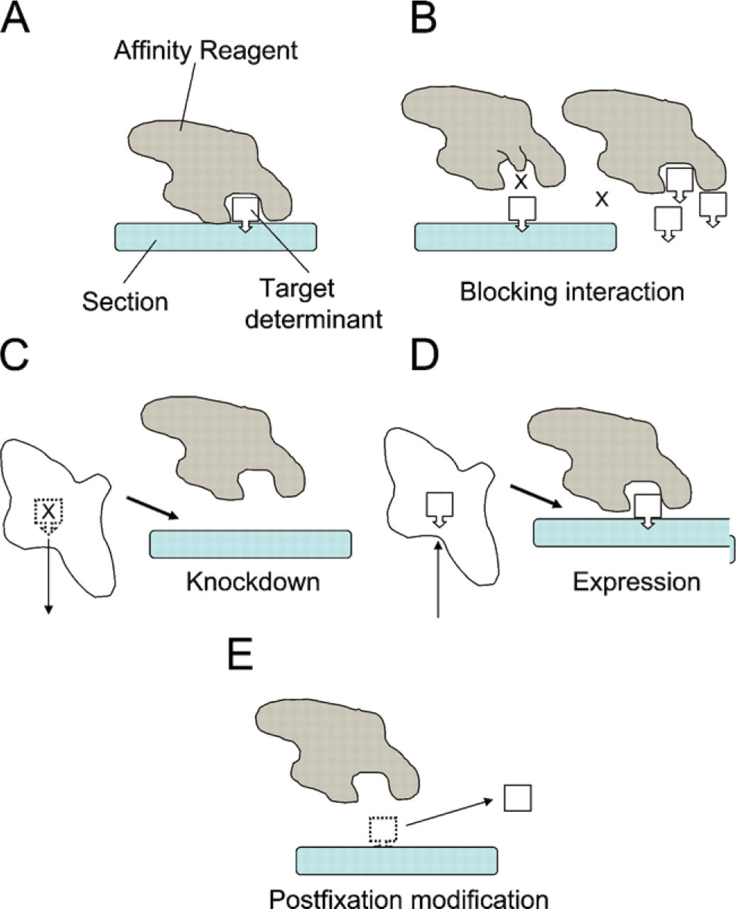
Reagent-based and specimen-based controls. (A) Terminology used in this report. The primary affinity reagent (Affinity Reagent) becomes associated with a target determinant (carried on a target component molecule), which is embedded within the ultrathin section (Section). (B) Reagent-based controls. Left: Interactions of reagent with target determinant can be blocked by modification (in this case mutation) of the binding site, thereby reducing labeling. The affinity reagent is otherwise similar in amino acid sequence, ensuring nonspecific interactions can be preserved. Right: Excess soluble target determinants are introduced into the system and compete for binding of target determinants in the section. In this type of control, effects of the point mutation or competition for binding can be independently verified using biochemical tests for specificity. (C-E) Specimen-based controls by modification of the target component determinant. In C, target determinants are reduced by restricted or deleted expression, which is ideally verified by independent biochemical means. In D, target components carrying target determinants are introduced to the system in this case by inducing expression, although a variety of other methods could be used (see text). Often convenient determinants (such as epitope tags) may be introduced to the target components to facilitate labeling. Preferably, in this type of system, the expression of the endogenous target may need to be suppressed, and the introduced target should be at similar levels to that of endogenous. In E, the determinant is modified chemically before labeling in order to modify the interaction of the affinity reagent with the determinant. In this case, the section has been exposed to an enzyme, which modifies the determinant by cleaving specifically the bond between the determinant and the target component. A good example in this case is the localization of phosphotyrosine (pTyr) using specific antibody. The section is exposed to a phosphatase with specificity for this epitope, and the section is then labeled using the phosphotyrosine antibody. Reduction in the labeling indicates specific labeling for the pTyr.

Multiple non-covalent interactions ensure tight and specific binding of the target molecules embedded in the electron microscopic (EM) section, and also two types of nonspecific interactions occur. First, there are nonspecific interactions with non-target components in the ultrathin sections, which can be manifested as binding to any organelle profile (Momayezi et al. 2000). The classic sites for the most intense labeling of this type are profiles of the nucleus, mitochondria, or peroxisomes (Roth et al. 1981; Nanci et al. 1985; Lucocq et al. 1987); the evidence that this binding is to non-target components comes from the resistance of this nonspecific labeling to substitution of the specific primary antibody by nonspecific antibodies in the labeling system. The biochemical/biophysical basis of these interactions appears not to have been analyzed in any great detail, but is likely due to combinations of the same forces that ensure specificity (discussed earlier). Consistent with this, nonspecific labeling of this type may be reduced by appropriate dilution of the primary affinity reagent (dilution), high salt conditions, detergents, or inclusion of carrier proteins [e.g., BSA, ovalbumin, fish skin gelatin, or non-immune serum; see Lucocq et al. (1986) and Griffiths (1993)]. Nonspecific binding may also occur when aldehyde groups, introduced through crosslinking fixation, crosslink the reagents to the section, although there appears to be a general consensus that judicious use of aldehyde-blocking agents such as ammonium chloride and glycine can prevent this (Griffiths 1993; Scothern and Garrod 2008). A second type of nonspecific interaction occurs when the specific interacting domain of the affinity reagent binds to determinants resembling, but not identical with, the target determinant. These target determinants are then likely to be located in components that are not related to the target. Examples would be the binding of lectins or antibodies to oligosaccharides with the same terminal sugar residues but belonging to oligosaccharides/glycoproteins distinct from the target oligosaccharide/glycoprotein. The exact extent of this type of nonspecific interaction may be difficult to analyze, but could be addressed using the knockdown/knockout approach described later. Finally, off-target labeling might occur when determinants identical to those found in the target component may be present in macromolecules unrelated to the target. One rare example from the literature is a monoclonal antibody that binds strongly to a sequence of amino acids occurring in protein(s) unrelated to the target (Nigg et al. 1982). This effect is less likely to be observed with polyclonal antibodies. Another well-known instance would be the occurrence of identical oligosaccharide chains on glycolipids and glycoproteins. Since its inception, a variety of approaches have been used for evaluating specificity in on-section immunogold-EM. These strategies are focused on two main elements of the labeling process: these are the labeling reagents and the specimen itself.

Analyzing Specificity: Reagent-based Controls

One popular way to perform a control for nonspecific interactions is to omit the affinity reagent altogether, but this might not reproduce levels of nonspecific labeling due to sticking to various organelles. A better approach is to substitute an affinity reagent with similar composition but with diminished or absent specific binding activity. This reagent can be an antibody of the same class as the primary reagent, but which lacks specificity for the antigen of interest, or a preimmune serum. However, a more focused method is to use an affinity reagent that has been modified in structure at the target-binding site (Figure 1B, left). This can be achieved chemically, although more often a mutated form of the affinity reagent is used. A recent example from our own studies is the use of mutated pleckstrin homology (PH) domains lacking crucial residues responsible for binding to the phosphoinositide. The PH domain of TAPP1 was used to localize the minor inner leaflet phosphoinositide PtdIns 3,4 P2, and the control was a mutated TAPP1 molecule that had a single amino acid substitution in the head group–binding site (Watt et al. 2004). In that study, there was a reduction in the labeling over a range of organelles. Crucially, this type of control does not distinguish binding of affinity reagents to determinants that are found in non-target macromolecules. Another related reagent-based control is to introduce excess soluble target determinant into the binding reaction (Figure 1B, right) (Roth and Wagner 1977; Bendayan 1981). In this case, the control is likely to inhibit binding to determinants found in off-target and in on-target components.

Thus, there is a range of reagent-based approaches, which examine the specificity of labeling, but these approaches focus on the affinity reagent itself rather than the target component. In fact, no amount of hard work at the level of the affinity reagent can define the specificity for the target component per se–-this can be examined effectively only at the level of the target component itself.

Analyzing Specificity: Specimen-based Controls

In this case, target components are either modified or up/downregulated selectively, most often before fixation of the living cell or tissue (Figures 1C and 1D) or more rarely after fixation by modification of components in the section (Figure 1E). Verification of the modification or expression level can, in many cases, be achieved by using independent biochemical methods such as immunoblotting, and it is much easier to achieve on living cells than after fixation. Thus, any change in labeling is likely to be related to the target component. There are broadly three approaches for modifying the target components to determine specificity of the labeling.

Downregulation of Target Components in Cells Before Fixation, After downregulation of the target component/determinant, there is a reduction of signal, indicating specificity (Figure 1C). One approach is to knockdown target expression using hairpin RNA (shRNA) or small inhibitory RNA (siRNA) that are usually only partially effective. A preferred approach is to knockout the gene in genetically tractable organisms such as yeast, Caenorhabditis elegans, or mice (Chan et al. 2009; Garraway et al. 2009; Li et al. 2009; Matters et al. 2009; Gawden-Bone et al. 2010), which ablates expression altogether, although viability of the organisms generated is a potential problem. One possible problem with these approaches is the secondary modification of cell function due to absence of the target components of interest, which could affect cell viability, localization, and/or metabolism or even modify the structure of compartments, thereby, affecting the extent and/or interpretation of any signal reduction. There is also the problem of compensatory upregulation of functionally linked cellular components. Theoretically, perhaps the best approach to counter these problems might be expression of proteins mutated to ablate binding of the primary affinity reagent, the so-called knockin, discussed later (Zhang et al. 2007; Tong et al. 2009). Another way to avoid the effects of reduced expression is to carry out chemical modification of the target component after fixation, most often on the surface of the section (discussed later).

Introduction of Target Components Into Cells.

Target components can be introduced into cells using genetic expression methods (Figure 1D) via microinjection (Idrissi et al. 2008), viral infection (Griffiths et al. 2001), or uptake by means of endocytosis (Boukour et al. 2006). One difficulty here is the effect on cell function before fixation and mislocalization due to overexpression. This can be minimized by the introduction of an epitope-tagged molecule to which antibodies are available combined with careful titration of expression to attain levels that are comparable to the endogenous protein. A large number of epitope tags have been applied in immuno-EM, but relatively few have been used reproducibly. These include FLAG, HA, myc, and GFP (Andjelkovic et al. 1997; Currie et al. 1999; Prior et al. 2001). The best tags will allow detection by the labeling system at low expression by using antibodies/binding reagents that produce low-noise/nonspecific staining when used at concentrations that can detect the target component of interest. One commonly used tag is GFP, which enables live cell imaging and correlative microscopy to be done (Keene et al. 2008). Good commercially available antibodies against GFP provide virtually no signal on non-expressing cells, allowing even widely distributed pools of antigen to be detected. A further refinement is the preparation of cells expressing knockdown-resistant epitope-tagged proteins in combination with knockdown of the endogenous proteins (Zhang et al. 2007).

Modification of Target Components in the Section.

An example for this approach is to use an enzyme with strict specificity for the target determinant (Figure 1E). The enzyme might be used to add additional components to the substrate, but most often will be used to degrade its substrate. Note that, in either case, the specificity of labeling is dependent on the specificity of the enzyme for the target.

A recent example from our own work is the application of purified catalytic domain of a tyrosine phosphatase on the surface of the section to determine the specificity of the labeling using an antibody raised against phosphotyrosine (Gawden-Bone et al. 2010). Here, two sequential sections are processed identically, except that one is preincubated with concentrated phosphatase solution before labeling with the antibody. The reduction in labeling is then an indication of the specificity of the labeling for pTyr (Gawden-Bone et al. 2010). Another example of this type of control is the use of N-linked oligossacharide processing enzymes such as glycosidase, endoglycosidase-H and endoglycosidase-F, and PNGase-F to control for the specificity of lectin- and oligossacharide-binding antibodies (Lucocq et al. 1987). An example of adding a target determinant comes from the same study by using galactosyltransferase to create new terminal galactose residues on terminal N-acteyl glucosamine residues situated in oligosaccharides located in the ultrathin section (Lucocq et al. 1987). Notice that, although the enzymes might be narrowly specific for the target determinant, this type of control may not distinguish between different components carrying the same target, and it is difficult to confirm by independent means that there has been a modification of the target determinant.

Approaches for Quantitative Evaluation of Labeling Specificity

Basic Concepts.

Ultrathin sections are extremely small samples of the animal, organ, or cell cultures. Precise quantitative estimates of gold particle labeling are dependent on the use of multistage schemes for sampling individuals, organs, slices, blocks, sections, and micrographs/fields (Lucocq 2008; Mayhew and Lucocq 2008). At each sampling stage, random sampling is recommended because it ensures acquisition of data that is minimally biased. However, a helpful modification to random sampling in many heterogeneous biological systems is systematic, uniform, random sampling, which can provide improved efficiency and is now the technique of first choice. In systematic random sampling, a regularly spaced array of samples is placed at random within the sample. For example, when sampling a tissue for EM, the positions of the blocks are taken systematically with constant distance between them and the first block is positioned at a random location. A typical application of the multistage sampling scheme is detailed in published reviews (Lucocq 1994,2008; Mayhew and Lucocq 2008). At the bottom end of this sampling scheme lies the electron-dense gold particle labeling used to “locate” the primary affinity reagent. A number of stereological estimators for labeling distribution and labeling density over compartment/organelle profiles are known (Griffiths 1993; Lucocq 1994,2008; Mayhew et al. 2009); these include the point counting for profile areas and line intersection counting for profile boundaries that are used here (Weibel 1979; Howard and Reed 1998). Gold particle labeling may also be quantified.

As already discussed, the total raw number of gold particles counted in any one labeled section when the target component is present at normal expression levels, Ng(+), is composed of specific, Ng(s), and nonspecific, Ng(ns), labeling. Another reason that the number of gold particles does not report directly on the number of target components is because the labeling efficiency (gold particles per target component) can vary (Lucocq 1994). This variation might be due to a number of factors, including stoichiometry of the labeling sequence, variation and effects of crosslinking, different posttranslational processing of the target, or variable penetration of labeling reagents into the section. Under normal conditions of immuno-EM, these effects are not controlled, and specialized experimental protocols are required for estimating labeling efficiency. For the purposes of this report, we consider only the specificity of labeling density and labeling distribution. We do not discuss here the application of specific labeling quantification in labeling efficiency calculations.

In the case of reduced expression, the residual labeling after reduced expression (knockdown/knockout) Ng(-) is then the best available estimate of the nonspecific component of the labeling, Ng(ns) (this will often be a conservative estimate in the case of knockdown because expression is often not reduced completely).

Thus, Ng(+) = Ng(s) + Ng(ns).

And an estimate of Ng(s) = Ng(+) - Ng(−).

The fraction of labeling that is specific, f(s), is given simply by f(s) = Ng(s)/Ng(+).

Assessing Contribution of Specific Labeling to Labeling Densities.

A commonly used readout of gold labeling is the concentration, or density, over organelle or cell structure profiles, and our focus here is on the possible reduction in labeling density that occurs when the expression of a component is reduced or the amount of target in the section is reduced by on-section modification. Thus,

D (s) = D (+) - D (-)

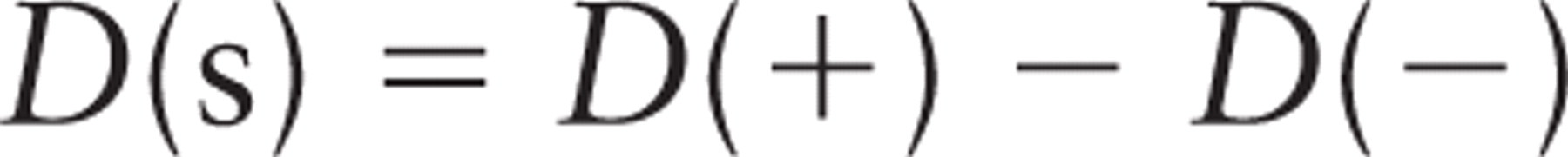
where D(+) is the density of labeling estimated over a compartment under the normal expression, D(-) is the density estimated on the same compartment in a specimen with reduced expression. D(s) is the specific labeling density, which is the difference between these densities. In the experimental systems, in which expression has been induced (++) rather than suppressed (-), an estimate of the specific labeling density is D(s) = D(++) - D(+). For reasons of simplicity, we focus only on the knockdown/knockout (reduced expression) case in this report.

The density of labeling can be expressed using Ng/A or Ng/B, where A is the area of organelle profiles and B is the length of membrane profiles assessed on the section. The counting of the number of gold particles (Ng) will involve appropriate sampling of gold particles, whereas A or B can conveniently be estimated using point counting or line intersection counting (Lucocq 1994,2008).

Importantly, for technical reasons under most circumstances, quantitative data on normal expression and reduced expression can only be obtained from different specimens/sections/fields, and therefore, an estimate of the specific labeling density is as follows:

Ng (s) / A (s) = (Ng (+) / A (+)) - (Ng (-) / A (-))

And when discrete stereological events (say point counts, P) are used, rather than absolute area/lengths, the labeling density can be assessed as a specific labeling index. Here the labeling is related to the number of point hits (gold particles per point) or line intersection counts (gold particles per intersection) as follows:

For point counts for profile area,

Ng (s) / \sum P (s) = (Ng (+) / Σ P (+)) - (Ng (-) / Σ P (-))

Or in the case of line intersections for boundary length,

Ng (s) / Σ I (s) = (Ng (+) / Σ I (+)) - (Ng (-) / Σ I (-))

The statistical precision of the specific labeling density estimate will depend on the precision of these ratio estimators. It has been found that, in the case of stereological estimates, a major determinant of precision is the variation between animals or cell cultures (Gundersen and Østerby 1981; Gupta et al. 1983). However, in our experience, knockdown using siRNA, induced expression, or on-section modification of targets are all additional major sources of variation in gold particle labeling estimates (our own unpublished data). Therefore, to improve precision in the final estimates, it is advisable to run at least three to five or more animals/experiments [see Howard and Reed (1998) for further discussion] and if possible to match normal and reduced expression samples as closely as possible, perhaps by using the same culture preparation or litter-mates and by processing the samples in parallel with ultrathin sections being incubated on the same droplets of reagents. In the case of on-section modification of target, the digestion/modification might be done on opposite sides of the same electron microscopic section (resin only) or on adjacent sections from the same block of embedded specimen.

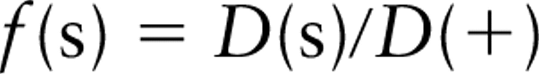
Estimating the Fraction of Labeling That Is Specific (Specific Labeling Fraction).

From the density estimates, an estimate of the probability that a gold particle counted in the raw (total labeling) data will be specific (f(s)) can be obtained from

f (s) = D (s) / D (+)

or from accessible counts on separate samples with normal and reduced expression

f (s) = (D (+) - D (-)) / D (+)

and by substitution and rearrangement

f (s) = 1 - ((Ng (-) \times A (+)) / (A (-) \times Ng (+))) .

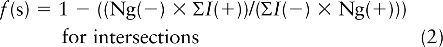
However, as noted earlier, the simplest scenario is when the densities can be estimated in relation to point counts or intersection counts. This gives a measure of intensity over each compartment considered. The difference in the intensities can then be expressed as a fraction of the intensity estimated for the test condition. Again, this fraction, the specific labeling fraction, is an estimate of the probability that labeling over a compartment will be specific:

f (s) = 1 - ((Ng (-) \times Σ P (+)) / (Σ P (-) \times Ng (+))) for point counts, and

f (s) = 1 - ((Ng (-) \times Σ I (+)) / (Σ I (-) \times Ng (+))) for intersections

The accuracy of this estimate over a particular compartment will depend on the number of gold particles and the number of point/line intersection hits. So for a compartment with fewer counted gold particles and with fewer counted point or line intersection hits, the precision of the probability estimate will tend to be lower than that if the counts are higher. On the basis of previous studies (Lucocq et al. 2004), it is recommended that ∼100–200 gold particles or probe hits are counted over the compartment.

Each element contributing to the specific labeling, i.e., D(+) and D(-), are ratio estimates–-i.e., the number of gold particles per point or intersection count. If data from only a single experiment are available, then the coefficient of error for the ratio estimate of density can be calculated (Cochran 1977) as long as individual sampling units (micrographs or scans) contribute to the final ratio. However, as already explained, major portions of the overall variation in signals are due to the variability between biological controls, and so it is advisable to run comparisons for control and test samples from at least three independent experiments.

In the example illustrated in Table 1, a single culture dish of cells from a randomly selected cell culture has been treated with siRNA for a membrane protein [reduced expression (-)] and another dish has been treated with scrambled siRNA as a control [normal expression (+)]. The cells were processed in parallel for immuno-EM, sectioned, and labeled, and the extent of membrane profiles in the various compartments was assessed using line intersection counting (Lucocq 1994). Twenty micrographs were taken from systematic, uniform, random locations, and particles/intersections were counted over all compartments. The results were used to estimate the gold particle density per intersection.

Table 1.

Specific labeling density and specific labeling fraction

	Ng(+)	I(+)	D(+) = Ng(+)/I(+)	Ng(-)	I(-)	D(-) = Ng(-)/I(-)	f(s)	D(s) = D(+) - D(-)
ER	49	80	0.613	13	95	0.137	0.777	0.476
NE	10	10	1	7	8	0.875	0.125	0.125
Golgi	7	11	0.636	7	13	0.54	0.154	0.098
SV	51	25	2.04	11	35	0.314	0.846	1.726
Mit	11	40	0.275	12	45	0.267	0.0303	0.008
EE	9	8	1.125	11	10	1.1	0.0222	0.025
LE	8	9	0.889	10	12	0.833	0.0625	0.056
PM	8	95	0.0842	9	109	0.0826	0.0195	0.0016
Total	153	278		80	327

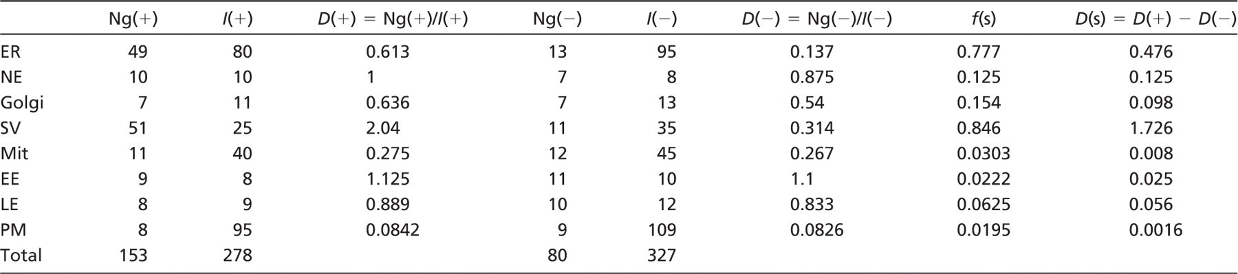
Two specimens, normal expression (+) and reduced expression (-), were fixed and embedded, and ultrathin sections were labeled for a membrane protein. Approximately 20 micrographs were taken at systematic uniform random locations (Lucocq 2008). Gold particle counts (Ng) and counts of intersections (I) between membrane profiles and lines of a test grid were made and tabulated. Densities were calculated as gold particles per intersection from D(+) = Ng(+)/I(+) for normal expression and D(-) = Ng(-)/I(-) for reduced expression. The difference in these densities D(s) represents an estimate of the density of specific labeling—the specific labeling density. The fraction of gold particles over each compartment that is specific, the specific labeling fraction, is given by D(s)/D(+) and is directly computed using Equation (2). D, labeling density; f(s), specific labeling fraction; D(s), specific labeling density; ER, endoplasmic reticulum; NE, nuclear envelope; Golgi, Golgi apparatus; SV, secretory vesicles; Mit, mitochondria; EE, early endosomes; LE, late endosomes; PM, plasma membrane.

The difference between the values obtained for full expression (D(+)) and reduced expression (D(-)) was expressed as a fraction (f(s)) of the value obtained at normal expression (D(+)). This fraction can be calculated easily from Equation (2). The results show that knockdown induced the largest reduction in labeling density over the secretory vesicles (SV), whereas there is also some reduction over endoplasmic reticulum (ER) and nuclear envelope (NE). The specific labeling fraction, f(s), is highest over SV (0.85) followed by ER (0.77), Golgi membranes (Golgi; 0.15), and NE (0.13). From this analysis, there is at least an 85% probability that a gold particle labeling a secretory granule is specific. The “at least” qualification is because the knockdown is unlikely to be complete (as determined by semi-quantitative western blotting), leaving the possibility of residual-specific labeling. Thus, secretion granules have highest fraction of specific labeling followed by plasma membrane (PM) and ER. Over mitochondrial membranes, early and late endosomes or PM less than 7% of the labeling was specific.

Estimating the Density of Labeling That Is Specific (Specific Labeling Density).

The specific labeling density (D(s)) becomes the best available estimate of the relative local concentration of the target within the caveats related to labeling efficiency discussed earlier in Basic Concepts. The specific labeling density (D(s)) is calculated simply from the difference in the densities D(+) and D(-) as in Equation (1), and from the synthetic example already discussed, the results are expressed in Table 1 (far right column). This analysis shows that the highest concentration of specific labeling is present over the SV. On the basis of normal expression (raw gold particle counts), the early endosomes had a substantial labeling density (1.13 gold particles/intersection), representing 55% of the density over SV. However, now the early endosomes have a much reduced specific labeling density (0.025 gold particles/intersection), representing only 1.4% of the SV density. Again by this measure of specific labeling, mitochondria are essentially unlabeled. Overall, the data show that major concentrations of specific label are found over SV and ER, and weakest label is found over mitochondria, endosomes, and PM.

Specific labeling density identifies those individual compartments that have the highest concentration of specific label. However, it is also possible to analyze the data across the compartments to determine whether the reduced expression produced a statistically significant difference in the labeling distribution and what the distribution of specific (real) label over a range of cell compartments will be.

Assessing the Statistical Significance of Labeling Distributions After Reduced Expression.

A simple way to compare two distributions is to prepare a contingency table and use the χ 2 test to determine significance of differences (Mayhew et al. 2003,2009; Mayhew and Lucocq 2008). This can be applied to the two sets of gold particle counts and is especially useful in the early stages of an investigation or for rapid screening of data generated from two experimental conditions. Densities are not calculated and intersection points or area point counts are not used. The example is illustrated in Table 2 and uses the data taken from Table 1.

First, the raw gold particle counts under normal expression and reduced expression are summed and inserted into the Table (Totals, column 3). Next, these summed counts are used to calculate the expected number of gold particles in each compartment (Exp), as if both sets had come from the same population. For example, the summed counts for ER divided by the total of summed counts (62/233) provides an estimate of the expected proportion over the ER. Next, the expected number of gold particles over the ER is computed by multiplying this proportion (62/233) by the total gold particles counted for the normal expression set ((62/233) × 153 = 40.71) and by the total number of gold particles for the reduced expression set ((62/233) × 80 = 21.29). Using the raw counts and the expected value for each compartment, it is possible to calculate a χ 2 value for each compartment in the case of the normal expression (χ 2 (+)) and the reduced expression (χ 2 (-)). In this case, the sum of the χ 2 values for all compartments is 27.6, and for (k −1)(r −1) = 7 degrees of freedom, this is highly significant with p<0.005 (k = number of columns and r = number of rows). Furthermore, if the individual χ 2 values are examined, the hot spots for differences between the normal and reduced expression conditions can be identified. It is important to point out that the highest χ 2 values may arise if the test compartment has either a higher or a lower value than the expected value. Notice that there are restrictions on the use of the χ 2 test. It is recommended that none of the categories has an expected value of 0 gold particles and not more than 20% has an expected value of less than 5. If these conditions apply, then categories can be “pooled” to increase the number of gold particles counted.

Table 2.

Comparing labeling distributions in normal expression and reduced expression

	Obs Ng(+)	Obs Ng(-)	Totals	Exp Ng(+)	Exp Ng(-)	Specificity index	χ 2 (+)	χ 2 (-)	χ 2 total
ER	49	13	62	40.71	21.29	0.593	1.69	3.23	4.91
NE	10	7	17	11.16	5.84	-0.304	0.12	0.23	0.35
Golgi	7	7	14	9.19	4.81	-0.695	0.52	1.00	1.52
SV	51	11	62	40.71	21.29	0.736	2.60	4.97	7.57
Mit	11	12	23	15.10	7.90	-0.791	1.11	2.13	3.25
EE	9	11	20	13.13	6.87	-0.917	1.30	2.49	3.79
LE	8	10	18	11.82	6.18	-0.941	1.23	2.36	3.60
PM	8	9	17	11.16	5.84	-0.825	0.90	1.71	2.61
Total	153	80	233	153	80		9.45	18.13	27.6

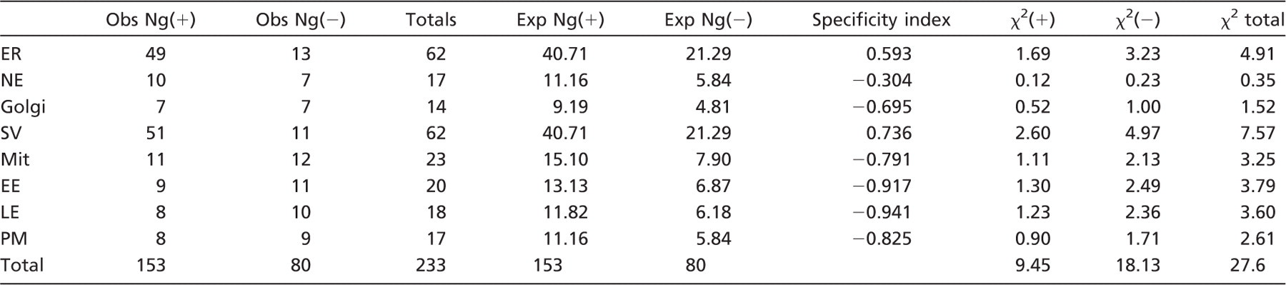
Data presented are derived from that presented in Table 1. Only gold particles are considered here. Gold particle counts from the two conditions are summed (Totals). The totals are used to estimate the total number of expected gold particles over each compartment as if the two counts came from the same population. For example, for ER, the expected value for the normal expression would be (62/233) × 153 = 40.71. For each condition and compartment, the expected value can be compared with the observed value as a χ 2 statistic of which the sampling distribution is known for different degrees of freedom. The formula for the χ 2 statistic is (Obs - Exp) 2 /Exp, with degrees of freedom df = (k - 1)(r - 1), where r is the number of rows and k is the number of columns. The df in this case is 7. The partial χ 2 statistic is presented and summed. The table of χ 2 values for the overall value 27.6 for df = 7 shows p<0.005, i.e., the two distributions come from the same population. To further analyze whether large χ 2 values come from a compartment with excess or lower than expected specific label, a specificity index is computed from (Obs(+)/Exp(+)) - (Obs(-)/Exp(-)). If positive (with values typically between 0 and +2), this index suggests a prominent χ 2 value is due to the accumulation of specific label in this compartment (see text for details). Note that the χ 2 and specificity index are most sensitive if compartments containing nonspecific labeling have been included in the analysis. Obs, observed value; Exp, expected value.

To aid in identifying compartments with possible specific labeling a specificity labeling can be computed, which represents the difference in the ratio of observed (Obs) to expected (Exp) values for the normal and reduced expression. For example, in the case of ER, the ratios are Obs Ng(+)/Exp Ng(+) = 49/40.71 = 1.204 and Obs Ng(-)/Exp Ng(-) = 13/21.29 = 0.61. The specificity index (1.204 - 0.61) is therefore +0.593, indicating more labeling over that compartment than expected from the pooled data. On the other hand for PM, the ratios are Obs Ng(+)/Exp Ng(+) = 8/11.16 = 0.76 and Obs Ng(-)/Exp Ng(-) = 9/5.84 = 1.54. The specificity index in this case is therefore −0.825, indicating less labeling than expected over that compartment. Simply put, when this index is positive, it indicates that the normal and reduced expression values are higher and lower than the expected values, respectively, and the specific labeling is less likely to be found over that particular compartment. Conversely, if the specificity index has a negative value, this indicates that specific labeling is less likely to be present over that compartment. Overall, the results show that the major contributors to the χ 2 value are the ER and the SV and that both of these compartments are labeled more than expected by comparison with the pooled distribution of gold particle counts.

Calculating Labeling Distributions: Specific Labeling Over a Range of Compartments.

One of the most important uses of gold particle labeling data is the evaluation of target component distribution by assessing the proportion of total labeling that is situated over each compartment. So far we have considered how to compute the probability that a gold particle situated over a cellular compartment is specific and the estimation of specific labeling density; also, we have compared two distributions using χ 2 analysis. The next section discusses how to compute the distribution of specific labeling using the specific labeling density data. The principle is to correct the observed raw counts over each compartment obtained under normal expression. This uses the estimate of specific labeling density as a multiplier that is applied to the estimator of compartment/structure (in this case the intersection counts) to find the number of specific gold particles over each compartment. For example, in Table 3 (which uses the data from the synthetic experiment in Table 1), the specific labeling density (D(s)) can be multiplied by the intersection counts obtained from the normal expression experiment (I(+)) to give the number of specific gold particles (Ng(s)). Using this data, the fraction of total specific gold particle label over each compartment can be computed and expressed as a percentage value, Freq(s) %, and compared with the percentages using the gold particle counts at normal expression, Freq(+) %. The results show that some compartments (mitochondria, early and late endosome, and Golgi) collectively appear to contain a significant fraction of the total labeling (23%) at normal expression, but after correction for specific labeling, they appear to contain much smaller proportion of label (3.8%). Now the only two compartments with substantial proportions of the label are the SV (50.9%) and the ER (44.9%). These compartments hold the vast majority of the labeling for this cellular component.

Simple Illustrative Example

The methods discussed earlier are brought together in the simple example illustrated in Figure 2 and Table 4. For reasons of simplicity and clarity, we show data from a single pair of microscopic fields with very low counts of gold particles and very low counts of intersections. In reality, there would be perhaps 20 or more microscopic fields and a 100 or more gold particles/intersections. In this experiment, the expression of a membrane protein has been reduced from normal expression (+) using siRNA (-), and the two specimens were fixed processed, sectioned, and immunogold-labeled for this particular protein. Again for simplicity, the gold particles are counted over three compartments: the PM, NE (shown here as a single membrane), and ER. The array of test lines was applied with random position and random orientation in relation to the underlying specimen/structure profiles. Intersections with the compartment membranes and the gold particles were counted for each condition. Notice that, because the numbers of counts and gold particles in this example were relatively low, the χ 2 analysis was not carried out.

Table 3.

Calculating the distribution of specific labeling across cellular compartments

	Ng(+)	I(+)	D(+)	Ng(-)	I(-)	D(-)	D(s) = D(+) - D(-)	Ng (s)	Freq(s) %	Freq(+) %
ER	49	80	0.61	13	95	0.137	0.476	38.05	44.92	32.0
NE	10	10	1	7	8	0.875	0.125	1.25	1.48	6.54
Golgi	7	11	0.64	7	13	0.54	0.098	1.077	1.27	4.58
SV	51	25	2.04	11	35	0.314	1.73	43.14	50.9	33.33
Mit	11	40	0.28	12	45	0.267	0.0083	0.333	0.39	7.19
EE	9	8	1.13	11	10	1.1	0.025	0.2	0.24	5.89
LE	8	9	0.89	10	12	0.833	0.056	0.5	0.59	5.23
PM	8	95	0.084	9	109	0.0826	0.0016	0.156	0.18	5.23
Total	153	278	80	327			84.7	100	100

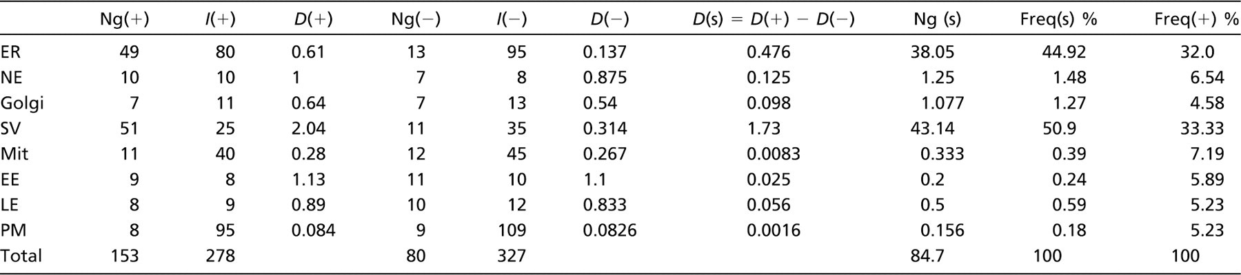
Data are from those displayed in Table 1. The number of gold particles labeling a compartment under normal expression conditions, Ng(+), is composed of specific Ng(s) and nonspecific elements Ng(ns)—the latter estimated as the number of specific gold particles labeling that compartment under reduced expression, Ng(-). The key is to estimate Ng(-) using the specific labeling density D(s), and the intersection counts for that compartment under the normal expression conditions, I(+); Ng(-) = D(s) × I(+). So for ER, Ng(+) = 0.476 × 80 = 38.1 specific gold particles. The number of specific gold particles can be calculated across all compartments, and the fraction is expressed as a percentage of total specific labeling for each compartment (Freq(s) %); these values are compared with that of the raw gold particle distribution obtained at normal expression levels (Freq(+) %).

The density of gold particles per intersection at normal expression, D(+) = Ng(+)/I(+), and at reduced expression, D(-) = Ng(-)/I(-), was calculated. For example, the values for the PM were 0.6 and 0.4 gold particles per intersection. The difference in these density estimates, specific labeling density D(s) = D(+) - D(-), was 0.2. As a fraction of the density at normal expression, the specific labeling fraction, f(s) = D(s)/D(+), was 0.2/0.6 = 0.33. The probability that a gold particle observed over the PM was specific was, therefore, 0.33. Next, the number of specific gold particles, Ng(s), labeling the PM were calculated by multiplying the specific labeling density, D(s), with the number of intersections counted over structures in normal expression condition, I(+). Ng(s) = D(s) × I(+), which for PM was 1.0. Overall, the results show the following: the specific labeling density was ∼2-fold higher over the ER compartment compared with the other compartments, and the probability that a gold particle represented specific labeling was highest (0.8) over ER compared to 0.33 over the other two compartments. The total number of specific gold particles over ER was 4.8 compared to 1 and 1 for PM and NE, respectively. Thus, the bulk of this antigen (70.6%) was present over the ER but, because of its extent, the density of specific labeling over the ER was not as marked when compared with specific labeling over the other two compartments.

Figure 2

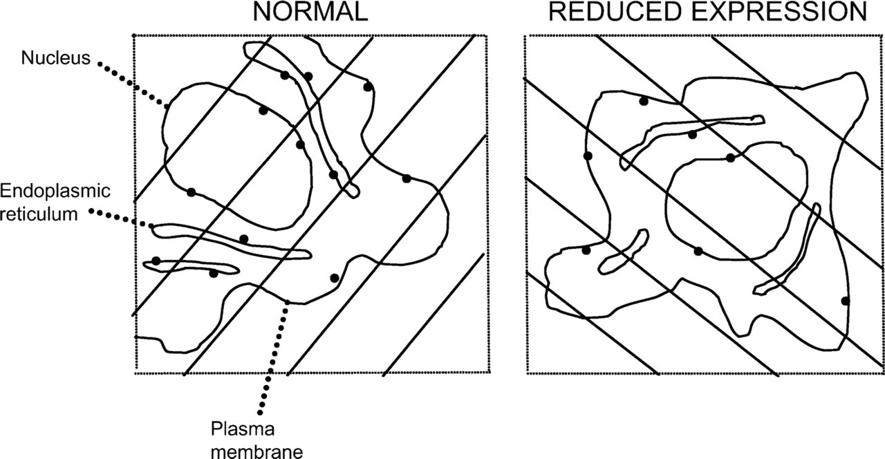
Assessing specific labeling–-simple illustrative example. Microscopic fields were sampled appropriately from ultrathin sections labeled for a membrane antigen–-one field from normal expression (NORMAL) condition and one from the reduced expression (REDUCED EXPRESSION) condition. Gold particles are indicated by black dots, and the cell compartment profiles were identified as indicated (for simplicity, nuclear envelope was drawn as a single membrane). Arrays of test lines were overlaid on the micrographs and intersections of one edge of each line with the compartmental membrane profiles were counted. The results are presented in Table 4 and discussed in the Results and Discussion section.

Table 4.

Quantitative assessment of specific labeling—simple example

	Ng(+)	I(+)	D(+)	Ng(-)	I(-)	D(-)	D(s) = D(+) - D(-)	f(s)	Ng(s)	Freq(s) %
PM	3	5	0.6	4	10	0.4	0.2	0.33	1	14.7
NE	3	4	0.75	2	4	0.5	0.25	0.33	1	14.7
ER	6	12	0.5	1	10	0.1	0.4	0.8	4.8	70.6

See text and Figure 2 for details and explanation of experiments. Briefly, the specific labeling fraction, f(s), is calculated from D(s)/D(+), and the number of specific gold particles per compartment, Ng(s), is calculated from D(s) × I(+).

Discussion

Here, we have used a systematic approach to the analysis of specificity in immunogold studies. Increasingly, this methodology is being used to pinpoint compartments/structures in which cellular components, particularly proteins, are concentrated. Although there is now a good base of techniques for assessing gold labeling per se (Lucocq 2008; Mayhew and Lucocq 2008), its value is somewhat diminished when attempts to analyze the specificity of the label are limited and the exact proportion of the observed label that can truly be assigned to indicate the component of interest remains unknown. Indeed, a review of recent studies from the PubMed online search tool using the term immuno EM indicated that target-based controls are still very much in the minority and also that controls are often not carried out at all (unpublished data). In response to this situation, our study now provides recommendations for controlling specificity in immuno-EM and suggests that specimen-based controls, i.e., those that modify the target component/determinant (preferably before processing for sectioning), are most useful, especially, if they can be supported using independent biochemical methods for measuring the extent of the modifications. We have illustrated how the density of specific labeling can be obtained using separate specimens: one with normal expression and the other with modified (usually reduced) expression of the target component. The difference between density estimates can be expressed as the probability that a gold particle labels the target. We also show how the statistical significance of the difference between the labeling distributions of the two specimens can be assessed using a combined contingency table/χ 2 analysis. Finally, our study describes how the distributions of specific labeling over a series of cellular compartments can be obtained, allowing calculation of percentages/fractions of specific label that lie over each compartment. Together, these methods have the potential to form a basis for future analysis of specificity in immuno-EM, forming part of an already established framework of methods that utilize appropriate sampling and minimally biased methods for structural estimation and gold particle counting.

References

Abramoff

Magelhaes

Ram

(2004) Image processing with ImageJ. Biophotonics International 11: 36–42.

Al-Amoudi

Chang

Leforestier

McDowall

Salamin

Norlén

Richter

, et al. (2004) Cryo-electron microscopy of vitreous sections. EMBO J 23: 3583–3588.

Andjelkovic

Alessi

Meier

Fernandez

Lamb

Frech

Cron

, et al. (1997) Role of translocation in the activation and function of protein kinase B. J Biol Chem 272: 31515–31524.

Bendayan

(1981) Ultrastructural localization of nuclei acids by the use of enzyme-gold complexes. J Histochem Cytochem 29: 531–541.

Bendayan

(2000) A review of the potential and versatility of colloidal gold cytochemical labeling for molecular morphology. Biotech Histochem 75: 203–242.

Bendayan

(2001) Worth its weight in gold. Science 291: 1363–1365.

Boukour

Massé

Bénit

Dubart-Kupperschmitt

Cramer

(2006) Lentivirus degradation and DC-SIGN expression by human platelets and megakaryocytes. J Thromb Haemost 4: 426–435.

Brändli

Parton

Simons

(1990) Transcytosis in MDCK cells: identification of glycoproteins transported bidirectionally between both plasma membrane domains. J Cell Biol 111: 2909–2921.

Chan

Arora

Bozavikov

McCulloch

(2009) FAK, PIP5KIgamma and gelsolin cooperatively mediate force-induced expression of alpha-smooth muscle actin. J Cell Sci 122: 2769–2781.

10.

Cochran

(1977) Sampling Techniques. London, Wiley.

11.

Cortese

Diaspro

Tacchetti

(2009) Advanced correlative light/electron microscopy: current methods and new developments using Tokuyasu cryosections. J Histochem Cytochem 57: 1103–1112.

12.

Currie

Walker

Gray

Deak

Casamayor

Downes

Cohen

, et al. (1999) Role of phosphatidylinositol 3,4,5-trisphosphate in regulating the activity and localization of 3-phosphoinositide-dependent protein kinase-1. Biochem J 337: 575–583.

13.

D'Amico

Skarmoutsou

(2008) Quantifying immunogold labeling in transmission electron microscopy. J Microsc 230: 9–15.

14.

Downes

Gray

Lucocq

(2005) Probing phosphoinositide functions in signaling and membrane trafficking. Trends Cell Biol 15: 259–268.

15.

Faraday

(1857) Experimental relations of gold (and other metals) to light. Phil Trans Soc 147: 145–181.

16.

Garraway

Inturrisi

(2009) siRNA-mediated knockdown of the NR1 subunit gene of the NMDA receptor attenuates formalin-induced pain behaviors in adult rats. J Pain 10: 380–390.

17.

Gawden-Bone

Zhou

King

Prescott

Watts

Lucocq

(2010) Dendritic cell podosomes are protrusive and invade extracellular matrix using metalloproteinase MMP-14. J Cell Sci 123: 1427–1437.

18.

Griffiths

(1993) Fine Structure Immunocytochemistry. Heidelberg, Springer.

19.

Griffiths

Roos

Schleich

Locker

(2001) Structure and assembly of intracellular mature vaccinia virus: thin-section analyses. J Virol 75: 11056–11070.

20.

Gundersen

HJG

Østerby

(1981) Optimizing sampling efficiency of stereological studies in biology: or “do more less well.” J Microsc 121: 65–73.

21.

Gupta

Mayhew

Bedi

Sharma

White

(1983) Inter-animal variation and its influence on the overall precision of morphometric estimates based on nested sampling designs. J Microsc 131: 147–154.

22.

Howard

Reed

(1998) Unbiased Stereology. Three Dimensional Measurement in Microscopy. Oxford, BIOS.

23.

Idrissi

Grötsch

Fernández-Golbano

Presciatto-Baschong

Riezman

Geli

(2008) Distinct acto/myosin-I structures associate with endocytic profiles at the plasma membrane. J Cell Biol 180: 1219–12132.

24.

Keene

Tufa

Lunstrum

Holden

Horton

(2008) Confocal/TEM overlay microscopy: a simple method for correlating confocal and electron microscopy of cells expressing GFP/YFP fusion proteins. Microsc Microanal 14: 342–348.

25.

Wang

Dinh

Ritter

(2009) Simultaneous silencing of Npy and Dbh expression in hindbrain A1/C1 catecholamine cells suppresses glucoprivic feeding. J Neurosci 29: 280–287.

26.

Londoño

Coulombe

Bendayan

(1989) Brief review on progresses in enzyme-gold cytochemistry. Scanning Microsc Suppl 3: 7–14.

27.

Lucocq

(1994) Quantitation of gold labeling and antigens in immunolabelled ultrathin sections. J Anat 184: 1–13.

28.

Lucocq

(2008) Quantification of structures and gold labeling in transmission electron microscopy. Methods Cell Biol 88: 59–82.

29.

Lucocq

(1993) Particulate markers for immunoelectron microscopy. In Griffiths

, ed. Fine Structure Immunocytochemistry. Berlin, Springer, Chap. 8, 279–302.

30.

Lucocq

Berger

Roth

(1987) Detection of terminal N-linked N-acetylglucosamine residues in the golgi apparatus using galactosyltransferase and endoglucosaminidase F/peptide N-glycosidase F: adaptation of a biochemical approach to electron microscopy. J Histochem Cytochem 35: 67–74.

31.

Lucocq

Brada

Roth

(1986) Immunolocalization of the oligosaccharide trimming enzyme glucosidase II. J Cell Biol 102: 2137–2146.

32.

Lucocq

Habermann

Watt

Backer

Mayhew

Griffiths

(2004) A rapid method for assessing the distribution of gold labeling on thin sections. J Histochem Cytochem 52: 991–1000.

33.

Matters

Harms

McGovern

Jayakumar

Crepin

Smith

Nelson

, et al. (2009) Growth of human pancreatic cancer is inhibited by down-regulation of gastrin gene expression. Pancreas 38:e151–161.

34.

Mayhew

Griffiths

Habermann

Lucocq

Emre

Webster

(2003) A simpler way of comparing the labeling densities of cellular compartments illustrated using data from VPARP and LAMP-1 immunogold labeling experiments. Histochem Cell Biol 119: 333–341.

35.

Mayhew

Lucocq

(2008) Developments in cell biology for quantitative immunoelectron microscopy based on thin sections: a review. Histochem Cell Biol 130: 299–313.

36.

Mayhew

Mühlfeld

Vanhecke

Ochs

(2009) A review of recent methods for efficiently quantifying immunogold and other nanoparticles using TEM sections through cells, tissues and organs. Ann Anat 191: 153–170.

37.

Momayezi

Kissmehl

Planner

(2000) Quantitative immunogold localization of protein phosphatase 2B (calcineurin) in Paramecium cells. J Histochem Cytochem 48: 1269–1281.

38.

Nanci

Bendayan

Slavkin

(1985) Enamel protein biosynthesis and secretion in mouse incisor secretory ameloblasts as revealed by high-resolution immunocytochemistry. J Histochem Cytochem 33: 1153–1160.

39.

Nigg

Walter

Singer

(1982) On the nature of crossreactions observed with antibodies directed to defined epitopes. Proc Natl Acad Sci USA 79: 5939–5943.

40.

Peters

Pierson

(2008) Immunogold labeling of thawed cryo-sections. Methods Cell Biol 88: 131–49.

41.

Prior

Harding

Yan

Sluimer

Parton

Hancock

(2001) GTP-dependent segregation of H-ras from lipid rafts is required for biological activity. Nat Cell Biol 3: 368–375.

42.

Roth

Bendayan

Carlemalm

Villiger

Garavito

(1981) Enhancement of structural preservation and immunocytochemical staining in low temperature embedded pancreatic tissue. J Histochem Cytochem 29: 663–671.

43.

Roth

Wagner

(1977) Peroxidase and gold complexes of lectins for double labeling of surface-binding sites by electron microscopy. J Histochem Cytochem 25: 1181–1184.

44.

Roth

Zuber

Komminoth

Sata

Heitz

(1996) Applications of immunogold and lectin-gold labeling in tumor research and diagnosis. Histochem Cell Biol 106: 131–148.

45.

Scothern

Garrod

(2008) Visualization of desmosomes in the electron microscope. Methods Cell Biol 88: 347–366.

46.

Siegel

Castellan

Jr (1988) Nonparametric Statistics for the Behavioral Sciences. 2nd ed. New York, McGraw-Hill.

47.

Skepper

(2000) Immunocytochemical strategies for electron microscopy: choice or compromise. J Microsc 199: 1–36.

48.

Tong

Pisani

Martella

Karouani

Yamaguchi

Pothos

Shen

(2009) R1441C mutation in LRRK2 impairs dopaminergic neurotransmission in mice. Proc Natl Acad Sci USA 106: 14622–14627.

49.

Watt

Kimber

Fleming

Leslie

Downes

Lucocq

(2004) Detection of novel intracellular agonist responsive pools of phosphatidylinositol 3,4-bisphosphate using the TAPP1 pleckstrin homology domain in immunoelectron microscopy. Biochem J 377: 653–663.

50.

Webster

Schwarz

Griffiths

(2008) Preparation of cells and tissues for immuno EM. Methods Cell Biol 88: 45–58.

51.

Weibel

(1979) Stereological Methods, vol. 1, Practical Methods for Biological Morphometry. New York, Academic Press.

52.

Zhang

Adams

(2007) Design and application of a shRNA-based gene replacement retrovirus. Methods Mol Biol 408: 211–221.

53.

Zuber

Fan

Guhl

Roth

(2005) Applications of immunogold labeling in ultrastructural pathology. Ultrastruct Pathol 29: 319–330.

Quantitative Assessment of Specificity in Immunoelectron Microscopy

Abstract

Keywords

Materials and Methods

Experiments and Statistics

Results

Specific and Nonspecific Labeling

Analyzing Specificity: Reagent-based Controls

Analyzing Specificity: Specimen-based Controls

Introduction of Target Components Into Cells.

Modification of Target Components in the Section.

Approaches for Quantitative Evaluation of Labeling Specificity

Basic Concepts.

Assessing Contribution of Specific Labeling to Labeling Densities.

Estimating the Fraction of Labeling That Is Specific (Specific Labeling Fraction).

Estimating the Density of Labeling That Is Specific (Specific Labeling Density).

Assessing the Statistical Significance of Labeling Distributions After Reduced Expression.

Calculating Labeling Distributions: Specific Labeling Over a Range of Compartments.

Simple Illustrative Example

Discussion

References