
Abstract
Objective:
To determine how different examination protocols with the use of transducers, of different bandwidths, and applied with varied tension to tendons would influence the sonographic study results.
Methods:
Thirty-one participants were divided into two groups, with one subject used for theoretical investigation (A) and the remaining participants (B = 30) forming the study cohort. Both sets of participants were examined with three different transducers (SL10–3, SL15–4, and SL18–7) as well as with variable loading on the Achilles tendon (relaxed, tensed, and loaded). The resulting coverage of the color map provided qualitative tendon stiffness and quantitative tendon stiffness values.
Results:
The estimated mean coverage extent, using elastographic color maps, produced by the three transducers was 98%, 98%, and 99%, respectively, in the relaxed state. Likewise, in the tensed state, mean coverage was 85%, 82%, and 77% in group A and 91%, 78%, and 71% in group B, respectively. Examining tendons that were loaded, the mean coverage was 68%, 42%, and 41%, respectively. The quantitative relaxed mean tendon elasticity values were 323, 366, and 393 kPa, respectively, in group A. Likewise, the relaxed mean values were 329, 341, and 358 kPa, respectively, in group B. The quantitative tensed mean tendon elasticity values were 413, 460, and 426 kPa, respectively, in group A. Likewise the tensed mean values were 412, 440, and 436 kPa, respectively, in group B.
Conclusions:
Varying the tendon loading significantly influenced the color map coverage, which governs the most reliable quantitative measurements on relaxed tendons. The best color map coverage was achieved using the transducer with the lowest frequency, regardless of the tension applied.
Tendons are frequently exposed to overuse and trauma, as they are subject to enormous loads resulting from muscle contraction and the lever mechanism formed by the joints. Continuous stretching leads to edema, microtears, and, eventually, tendon rupture.1–3 Although these types of degradation differ in biomechanical and biochemical mechanisms, they are similarly hypoechoic on gray-scale sonographic images and, therefore, often difficult or impossible to differentiate.4–6 Shear wave elastography (SWE) is increasingly being used for evaluating various musculoskeletal system constituents, including tendons and ligaments. The stiffness of a tendon is expected to reflect the nature of its degeneration, allowing possible differentiation between edema, tears, and microtears, leading to enhanced, patient-oriented treatment.7,8
Quantitative SWE imaging has received a great deal of attention over the past decade.7,9 Previous studies of shear wave speed variability in parenchymal tissues indicated that the estimated values differed with imaging depth in the case of phantoms as well as in the liver.
Furthermore, the speed values measured by two probes of different types and bandwidths but at the same depth also varied (probe SL10-2, Aixplorer [SuperSonic Imagine, Aix-en-Provence, France]; probe C5-1, EPIQ 5 [Philips Medical System, Best, the Netherlands]).10–13 Similar observations were made for muscle elastography, providing additional insight into the influences of load 14 and bone proximity to the inspected area15,16 for elasticity estimates.
These observations are consistent with the authors’ practical experience with Achilles tendon elastography. Unlike deeply located structures ie. some muscles, tendons and ligaments are superficially located and hence easily accesible for the ultrasonographic imaging. In some imaging cases, the factor of imaging depth can be minimized. However, there is a group of tendons located intramuscularly, where the influence of imaging depth cannot be avoided. When evaluating the Achilles tendon, this is not an influential factor. Further variability sources, (e.g., probe and tendon misalignment) can be minimalized by a trained, experienced sonographer using dedicated ultrasound equipment settings. Therefore, in this study, the focus was on investigating additional factors that influence Achilles tendon elasticity estimation, such as transducer bandwidth and the load exerted on the tissue. This problem was partially addressed in a study 17 in which the authors reported repeatability of both ex vivo and in vivo elastogram map generation. However, the tendons were examined under unloaded or barely loaded conditions only, and a single ultrasound transducer was used in the study.
In this study, rather than evaluating a large population of subjects, the decision was to repeat the examination multiple times on participants’ Achilles tendons and compare the results between the examinations. The tests were carried out using linear transducers of three different frequency bands, and the participants were examined in three different positions to vary the tendon tensile load.
Materials and Methods
Shear Wave Elastography
Using the SWE technique, shear waves are excited within the tissue by an acoustic radiation force, resulting from the absorption of focused high-intensity longitudinal waves. The shear waves propagate perpendicularly to the direction of the longitudinal wave beam, while low-intensity longitudinal waves are used for sonographic tissue imaging. Numerous images are acquired at a frame rate of up to 1 kHz; these images are subsequently correlated with each other to detect motion resulting from the propagated wave. If the amplitude of the perturbation is sufficient, shear waves are detected, and their speeds are calculated. The SWE process is illustrated in Figure 1.
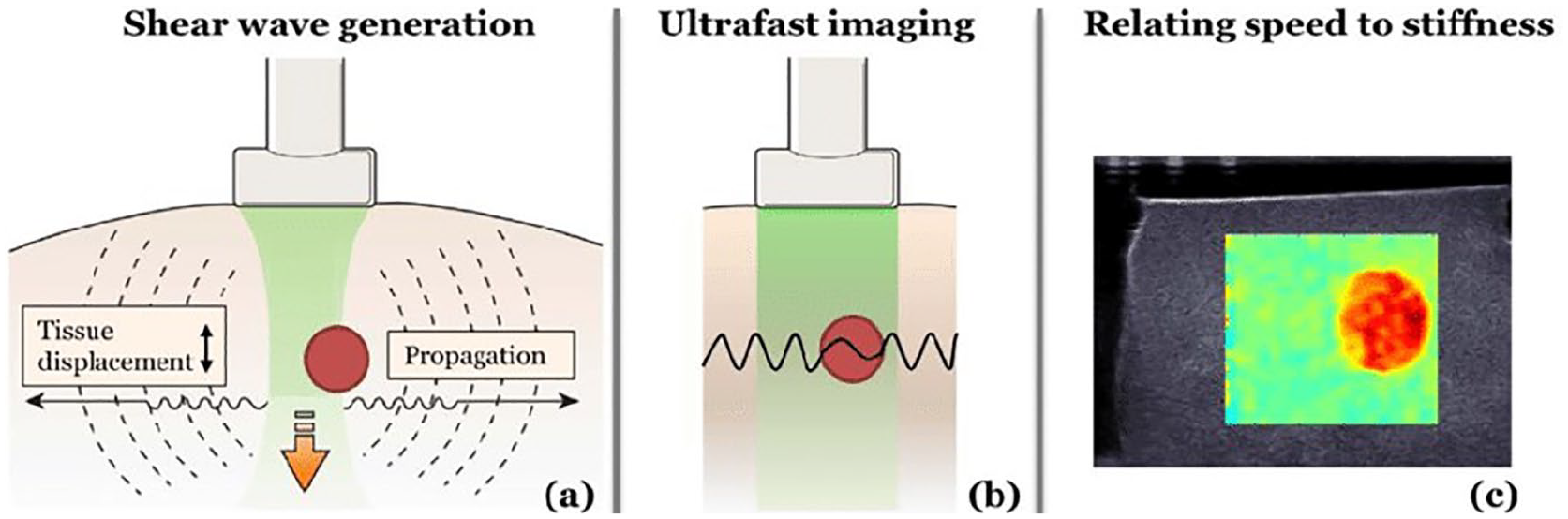
Shear wave elastography steps. A focused beam of longitudinal ultrasonic waves is absorbed and creates shear waves propagating perpendicularly to the beam (a). The shear wave speed and, hence, wavelength are affected by the local stiffness of the tissue (b). The final distribution of stiffness is created from the cross-correlation of images acquired in an ultrafast manner (c). Reprinted with permission from Maksuti. 18
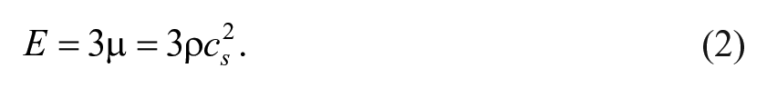
The speed of shear waves in tissues is a few meters per second. Assuming a nonviscous, elastic, nearly incompressible medium, it can be related to the shear modulus as follows 12 :

where cs is the shear wave speed, ρ is the density, and µ is the shear modulus. For soft tissues, it is assumed that Young’s modulus can be calculated using a simple expression as follows 13 :
Using this relationship, a map of the elasticity distribution is created and superimposed on the B-mode image. Depending on the implementation, the map can show shear wave speed in m/s or Young’s modulus in kPa.
Experimental Setup
The study protocol was designed according to the guidelines of the Declaration of Helsinki and Good Clinical Practices declaration statement. Special care was taken regarding personal data safety, and all images were anonymized before processing. Written informed consent for the publication of clinical details and anonymized clinical images was obtained from the Regional Bioethics Chamber (Krakow, Poland; no 158/KBL/OIL/2017). Written informed consent was also obtained from the participants for each experiment. The protocol for the entire study was approved by the authority of the clinic.
Experiments were divided into two parts. Part A was the first theoretical experiment conducted on a healthy 31-year-old woman. Part B consisted of measurements that were taken from the Achilles tendons of 30 patients between 20 and 36 years of age. The body mass indices of the subjects were comparable between the men (19 ± 1.2 kg/m2) and women (21 ± 1.5 kg/m2). To create controlled and steady conditions for the study, subjects with normal Achilles tendons were chosen for both experiments. The participants recruited included patients who were treated for conditions other than Achilles tendon problems and did not report any excessive sports activity, laborious work, or previous trauma to the Achilles tendons. Gray-scale sonographic images of the tendons in sagittal and transverse planes were carefully studied to ensure that no visible signs of Achilles tendon degradation were present. Criteria of exclusion included presence of scars, tendinosis, tendinitis, or partial rupture (including delamination). The measurements were acquired in the morning after overnight rest with no excessive walking activity in the morning (subjects traveled to the clinic using public or private transport). The plan for experiment A was as follows: the patient was asked to lie down on her abdomen on the couch with the foot in a relaxed position for repetitive probe alignment. Graduation was marked on the skin of the patient using a marker pen. The transducer was placed 10 mm above the calcaneal tuberosity. The measurements were obtained using three SuperLinear (SL; SuperSonic Imagine) transducers, with different frequency bands (SL10–2, SL15–4, and SL18–7). Repetitive measurements were taken with handheld probes one after another. Experiments were conducted in three different positions to apply different loads to the tendon and test its influence on the SWE measurements.
In group A, three different experimental settings were applied:
Patient was lying prone on the couch with relaxed tendon (relaxed Achilles group).
Patient stood with support of a walking frame (tensed Achilles group).
Patient stood on flexed toes with support of a walking frame (loaded Achilles group).
In each experimental setting (relaxed, tensed, and loaded), three transducers of different bandwidths were used: SL10–2, SL15–4, and SL18–7; therefore, nine experimental settings were examined. There were 30 measurements taken with each of the transducers for every patient position. A total of 270 measurements (9 × 30) were made in this experiment.
In group B (cohort study), 30 patients were examined, but two different experimental settings were used:
Patient was lying prone on the couch with relaxed tendon (relaxed Achilles group).
Patient stood with support of a walking frame (tensed Achilles group).
In this group of 30 patients, with each experimental setting (relaxed and tensed Achilles), three transducers of different bandwidths were used: SL10–2, SL15–4, and SL18–7. One measurement with each transducer was taken in each patient position. Six experimental settings were examined in this cohort for a total of 180 measurements (6 × 30).
B-mode images and elasticity maps of the tendon were obtained in the sagittal view, with the standard alignment of the transducer parallel to the tendon. The transducer setup was carefully monitored. While standing on their toes, the participants stabilized themselves by using an immobilized walker (walking frame), as shown in Figure 2.
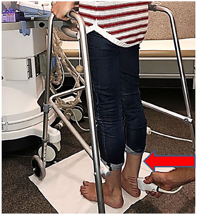
Demonstrating the experimental setup with the participant in the standing position. The transducer is aligned to the patient’s skin (red arrow) in the sagittal place for imaging.
In part B, measurements were made on the cohort of 30 patients. As described above, the experiment was performed using three Aixplorer (Supersonic Imaging) transducers (SL10–2, SL15–4, and SL18–7), which were handheld and placed 10 mm above the calcaneal tuberosity. For each patient, three measurements of local tendon stiffness were taken with each of the three transducers and evaluated from the local region of interest (ROI), referred to as a QBox. These measurements were based on the software provided with the ultrasound unit. In both experimental groups, the points for the three measurements were precisely set at the proximal part of the tendon (approximately 7 cm, 5 cm, and 3 cm above the calcaneal tuberosity), using calipers and bony landmarks.
The experiments were carried out using Aixplorer version 10.0 Aixplorer (SuperSonic Imagine). Images were collected using musculoskeletal protocol (MSK) presets (SWE optimization: standard; HD/frame rate: balanced; zoom: 120%; smoothing: 5; persistence: high). The shear modulus measurement was limited to 800 kPa, and the gain and power settings were kept constant across all the measurements.
Measurements were made on each patient in both the recumbent and standing positions. Numerical results are presented in table format (see Figures 3 and 4).
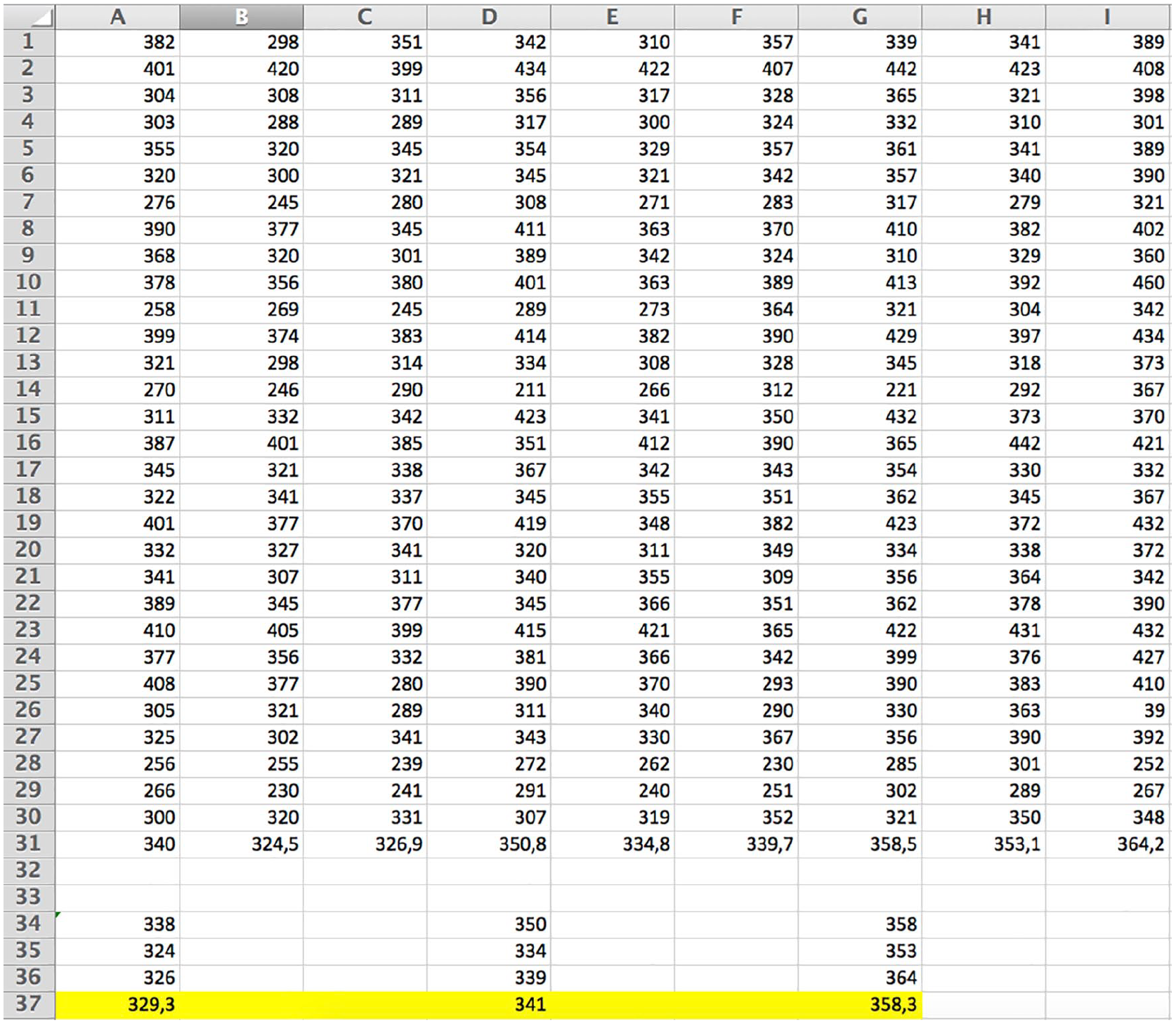
Numerical values of elasticity read from the Aixplorer QBox, with the transducer pointed on the relaxed Achilles tendon. Three measurements for each tendon obtained with SL10–2, SL15–4, and SL18–7 transducers are shown in the A, B, and C columns; D, E, and F columns; and G, H, and I columns, respectively. Mean values are presented below.
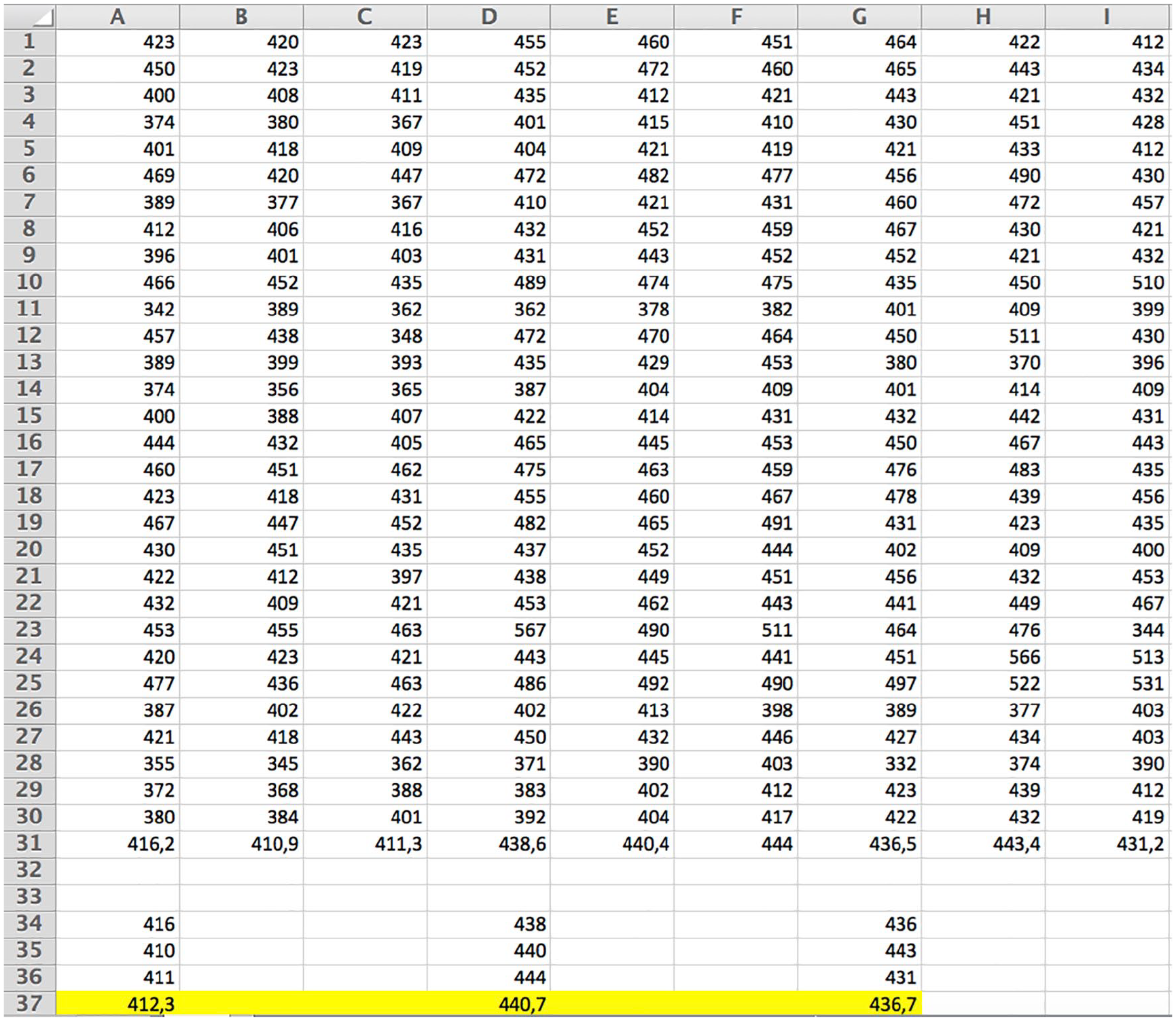
Numerical values of elasticity read from the Aixplorer QBox, with the transducer pointed on the tensed Achilles tendon. Three measurements for each tendon obtained with SL10–2, SL15–4, and SL18–7 transducers are shown in A, B, and C columns; D, E, and F columns; and G, H, and I columns, respectively. Mean values are presented below.
The quality of the results was assessed based on the computerized analysis of the color map coverage and consistency, which was verified in comparison to control data (MATLAB; MathWorks, Natick, MA). Statistical analysis was generated based on the statistical program, Statistica (Stat Soft 9.0). Data belonging to the proposed groups (made with low, mid, and high transducer resolution) were compared using unpaired t tests for each of the two parameters (namely, image coverage and mean elasticity) to the control (100% coverage of the color map and baseline elasticity estimated by transducers of different resolutions). Similarly, results were compared in the groups with measurements made in a chosen position.
Nine t tests were performed in total. The differences in results between the aforementioned groups and the control were assumed to be statistically significant when P < .005.
Data Processing
To precisely localize the tendon, both elastograms and raw gray-scale sonographic images were acquired, as illustrated in Figure 5. Two scenarios were used for investigation: first, a polygonal ROI was marked for analysis of a region of the image corresponding to the total tendon inspected using SWE. Moreover, four round ROIs, selected for evaluation of local stiffness, were distributed arbitrarily over the tendon ROI. The ROIs were placed on the gray-scale sonographic image where the tendon could easily be identified, and their coordinates were translated to the elasticity map.
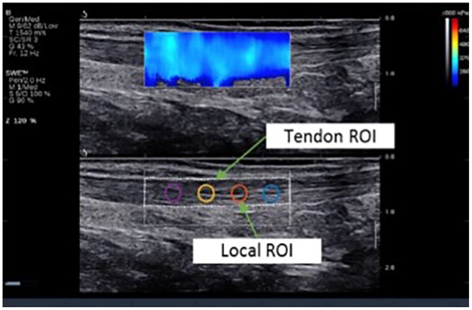
Tendon and local regions of interest (ROIs) used for processing. The sonographic image was taken during the standard examination with the subject in a prone, relaxed position with sagittal probe alignment.
To process the acquired images, a custom analysis program was created using the MATLAB environment (MathWorks). Statistics were calculated for both tendon and local ROIs. The first parameter was elasticity map coverage, computed as the ratio of the colored image area within an ROI to the total area of the ROI. Calculation of the percentage of the color map covering the gray-scale image was performed using ImageJ software (National Institutes of Health [NIH], Bethesda, MD) on the 8-bit converted tiff image after conversion of the RGB information to the brightness histogram as the mean of the RGB signal, with V = (R + G + B)/3, where V is brightness.
In the next step, the color map values were translated to elasticity values. For each ROI, the mean elasticity was calculated from the elastography map. The procedure was repeated for each of the 30 images, yielding a set of 30 sample means for each case. Finally, the sampling distribution was presented as a box plot.
Results
Elastogram Coverage and Mean Elasticity
In the first experiment, the interplay between elasticity map formation and load applied to the tendon was examined. As shown in Figure 6, the area of the tendon covered by the elasticity map decreased with increased load. This issue was observed in several experiments; however, it differed depending on the transducer used for the examination, as can be seen in a column-wise comparison of images presented in Figure 6. To evaluate the problem more closely, for each acquired image, the ratio of the area of the elasticity map to the area of the tendon ROI was calculated.
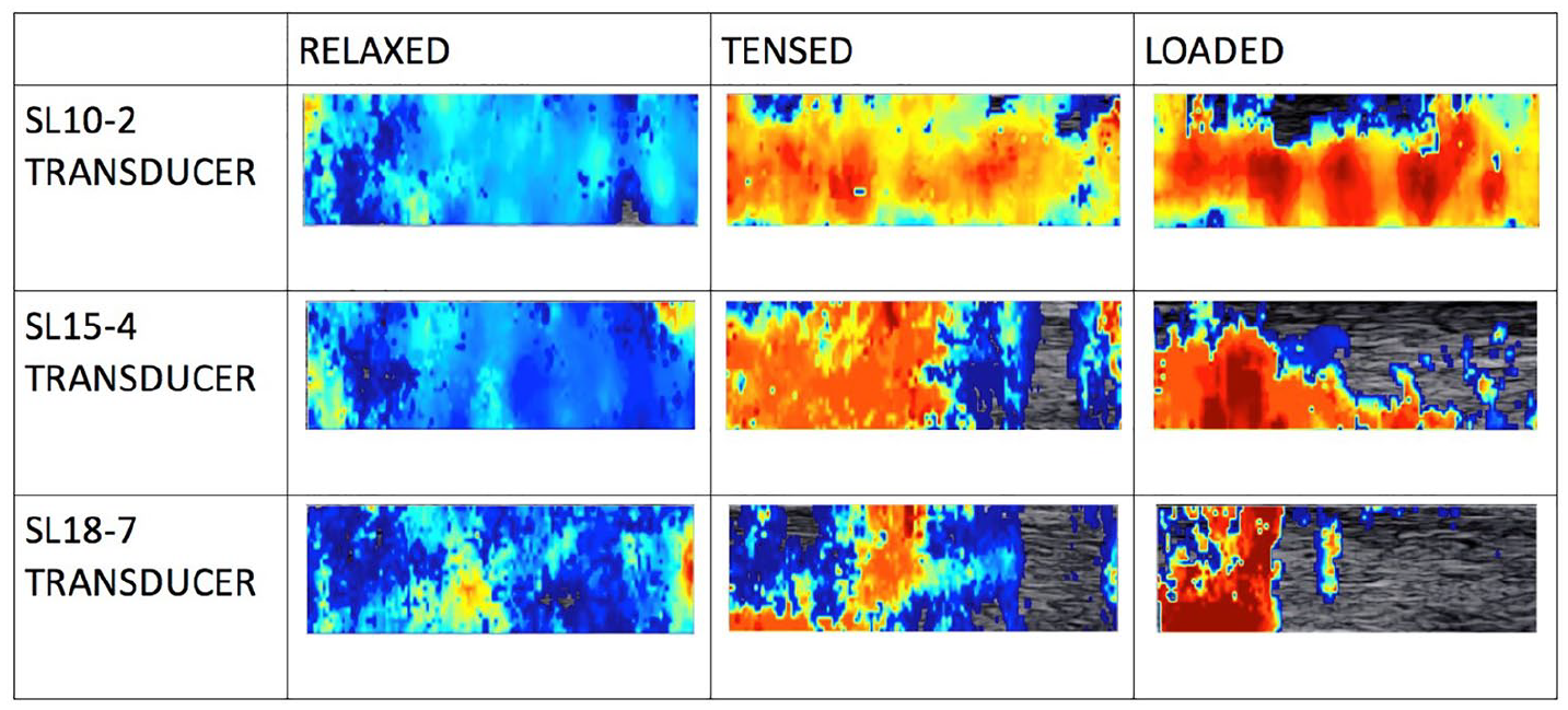
Elasticity color maps visualized within local regions of interest placed on the Achilles tendon. The maps were collected from the relaxed, tensed, and loaded Achilles tendon of the female patient (31 years old). Note the progressively reduced coverage on the color map as the tendon load increases and that the color expressions of stiffness are different for the various transducers.
As shown in Figure 7, in the relaxed condition, all transducers provided 100% coverage in almost all cases. When the tendons were tensed, a significant drop in coverage was observed. This can be explained by the fact that the displacement of the tissue resulting from wave propagation is inversely proportional to tissue stiffness and load. Therefore, increasing the tension may reduce the shear wave amplitude below the threshold detectable by the system. From Figure 6, it also can be concluded that elastogram coverage obtained with the SL10–2 transducer was superior to the coverage obtained using higher-frequency transducers. This can be explained by shear wave attenuation, which increases with frequency. The central frequency of the transducer generating longitudinal waves has a strong influence on the frequency of the generated shear waves. High-frequency longitudinal waves permit stronger focusing on smaller areas than low-frequency waves. Small focal points provide excitation at short wavelengths and hence high-frequency shear waves.
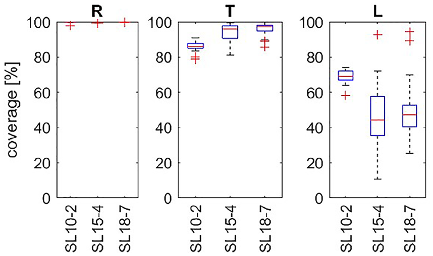
A box plot of the coverage of the elasticity map, within a tendon region of interest. Experiment A (multiplied measurements in one participant). R, T, and L denote the relaxed, tensed, and loaded tendon states, respectively. The transducer type is noted on the horizontal axis.
In the next step, the elasticity maps obtained during each repetition were subjected to estimation of mean stiffness. The resulting sampling distributions of the sample mean are presented in Figure 8 using box plots. In Figure 8 in the (R) condition, the outliers of elasticity values are increased significantly with increased frequency of the transducer (SL18–7 vs SL10–2 and SL15–4). Since the frequency of the transducer results in a higher shear wave frequency, this suggests that the shear waves in the tendon are subject to dispersion, which leads to a frequency-dependent velocity. 19 The results obtained, presented in Figure 8, for T do not support this hypothesis. Low elasticity values with high variance were obtained from the loaded tendon, as shown in Figure 8 (L); these results together with the results presented in Figure 7 (L) suggest insufficient excitation and/or sensing of the shear waves. E, noted on the vertical axis, indicates measured elasticity of the tendon.
Box plots of average tendon elasticity within the tendon region of interest made on the basis of multiple experiment made in the group A. The central line denotes the median; the edges of the box are the 25th and 75th percentiles. Points considered outliers are plotted as crosses, whereas whiskers extend to the most extreme values considered not to be outliers. R, T, and L denote the relaxed, tensed, and loaded tendon states, respectively. The transducer type is noted on the horizontal axis. E, noted on the vertical axis, indicates measured elasticity of the tendon.
In the experiments performed on the healthy subjects, a decrease in the color map coverage area was observed between the maps made with relaxed and tensed Achilles tendons. This was also noted for the different transducers used, such as SL10–2, SL15–4, and SL18–7.
The observed reduction in the coverage of the tendon image with color SWE did not influence readings of the experiments while ROIs were set on the area of the color map (a QBox was moved anteriorly and posteriorly on the set distance to the calcaneal tuberosity).
Local Elasticity
A similar procedure was performed for each circular ROI set within the tendon area analyzed in the theoretical experiment (group A). The elasticity map coverage within the local ROIs is presented in Figure 9. For all subjects, high average coverage was observed under the relaxed condition for all four local ROIs. However, in the case of a tensed tendon, a drop in the average coverage could be observed, and the mean elasticity map coverage was even smaller in the case of a loaded tendon, which was in good agreement with previous observations made for the total tendon area, as presented in Figure 7.
Coverage of elasticity maps within four local regions of interest on the participant in the tendon area.
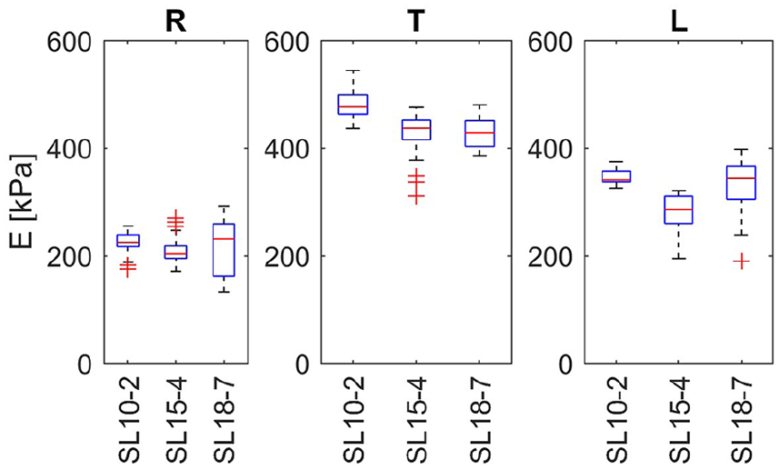
Reviewing the data in Figure 9, it can also be concluded that using the low-frequency SL10–2 transducer resulted in better performance in terms of elasticity map coverage than using the high-frequency transducer, SL18–7. Therefore, a final analysis was performed for different loading states using the SL10–2 transducer only. The results are presented as box plots in Figure 10. From the results presented in Figure 10, it can be seen that the elasticity variation rose with increased load. This is not the case in Figure 10, in which the tensed (T) position exhibited the smallest distribution of values. However, note that in Figure 10 (R) and (T), additional values appear that were classified as outliers. Much lower variability was observed among the women, as shown in Figure 10.
A box plot distribution of elasticity within selected local regions of interest obtained using the SL10–2 transducer from various loading positions for the healthy participant (group A). The central line denotes the median; the edges of the box are the 25th and 75th percentiles. Points considered outliers are plotted as crosses, whereas whiskers extend to the most extreme values considered not to be outliers. E, noted on the vertical axis, indicates measured elasticity of the tendon.
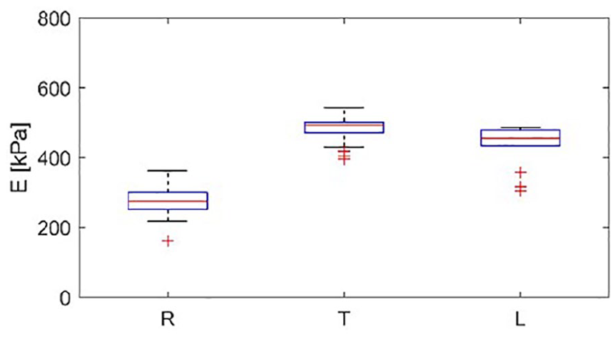
The combination of an increased load and high transducer frequency leads to reduced elasticity map coverage, which could make the results unreliable. Therefore, only results from the relaxed position are presented in Figure 11 next to box plots indicating the coverage quartiles of the elastogram map within the investigated ROI. In all cases, the results exhibit little variability regardless of the transducer used. For the men (subjects 1 and 2), the median elasticity value was close to 550 kPa. Similarly, for the healthy participant, as presented in Figure 11, the median values are slightly lower than those of the men; however, the low variability is maintained. The last analysis led to the conclusion that the most reliable and repeatable results among all experiments were obtained under the relaxed condition.
Box plots of the distribution of elasticity within local regions of interest in the relaxed position (R) made with the healthy participant. The central line denotes the median; the edges of the box are the 25th and 75th percentiles. Points considered outliers are plotted as crosses, whereas whiskers extend to the most extreme values considered not to be outliers. E, noted on the vertical axis, indicates measured elasticity of the tendon.
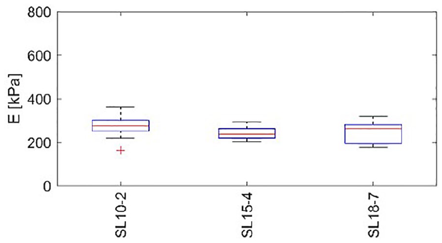
Part B with 30 healthy subjects was conducted as a “convenient experiment” on healthy participants in the recumbent position. Statistically different mean elasticity values were found between low- and high-frequency transducers with the relative difference not exceeding 30 kPa (Figure 12).
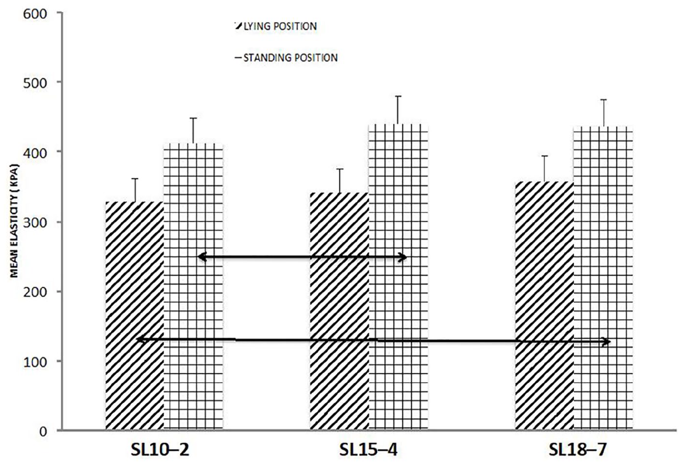
Changes in the mean elasticity values measured in the lying position (stripes) and standing position (bars) using different transducers. Double arrows point to statistically significant differences with P < .005.
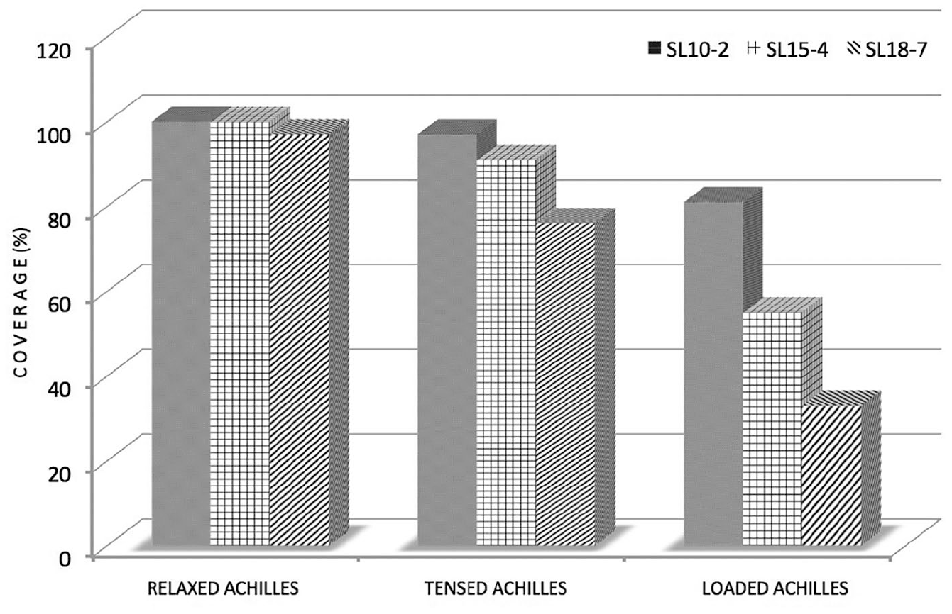
In the experiment conducted in the standing position, higher mean tendon elasticity values were recorded for the low-frequency transducer SL10–2 (412 ± 41 kPa vs 329 ± 32 kPa), middle-frequency transducer SL15–4 (440 ± 27 kPa vs 341 ± 31 kPa), and high-frequency transducer SL18–7 (436 ± 43 kPa vs 358 ± 51 kPa) (Figure 12). Coverage of the tendon with the color map was decreased by 9%, 22%, and 29% for SL10–2, SL15–4, and SL18–7, respectively, in comparison to 100% cover- age as assumed in the maps made using the relaxed Achilles tendon (Figure 13).
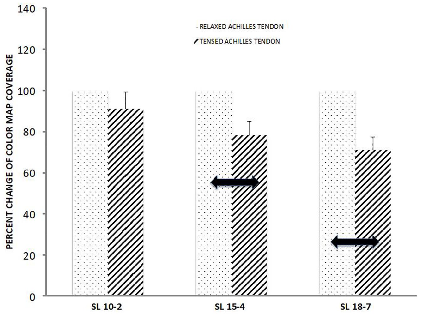
Percent change of the color map coverage of the tensed Achilles tendon examined using different transducers (SL10–2, SL15–4, SL18–7) in comparison to the control (the study was performed on the tensed vs relaxed tendon). Thick double arrows point to statistically significant differences with P < .005.
In part A, the group with the loaded Achilles tendon while standing on flexed toes was excluded for the following reasons. First, the theoretical part proved that in the loaded Achilles tendon, color map buildup was very limited for the high-frequency transducer. Second, the use of this technique for assessing Achilles elasticity in clinical practice is very improbable.
In both experiments (A and B), good interdata agreement was found [96% (Figure 8 and 12) and 92% (Figure 7 and 13)] for the elasticity data and elasticity map coverage, respectively).
Correlations between mean elasticity values were calculated in experiments A and B. A close correlation of 96% was noted. Correlations between mean elasticity map coverage in experiments A and B also were calculated. Again, a close correlation of 92% was found.
Discussion
These results demonstrate that the best color map coverage was achieved using the transducer with the lowest frequency, independent of the examined object’s tension. However, tension of the tendon was not neutral for the readings on the ultrasound equipment. The values measured using low-frequency transducers were considered trustworthy. In the highly loaded tendons tension readings were limited therefore recorded differences among transducers were insignificant. Values measured in loaded tendons were lower than those measured in tensed and relaxed tendons.
The concept and practical application of quantitative elastography is a clear milestone in the noninvasive analysis of biological tissues. In MSK applications, however, the lack of standardization of the technique causes inconsistency in the results obtained from different tendons and ligaments. In extreme cases, it is not possible to create color maps at all. In our daily work using SWE, we have found limitations related to the lack of measurement reproducibility. This is in agreement with other studies that addressed similar technical problems.10,17,20
The relatively small dimensions of examined structures are, at least in part, responsible for errors because in such cases, accurate transducer alignment requires a great deal of care from the examiner. The results can be affected by changes in the position of the joint and by slight probe movements caused by handheld operation (used in the majority of clinical situations). However, these factors do not account for some problems that arise even when examinations are conducted carefully.21,22
Complex viscoelastic properties of the tendon can influence the generation of elasticity maps at different stages: wave generation, detection, and translation of the wave speed to Young’s modulus. The viscosity creates attenuation, which results in wave dispersion; therefore, estimation of Young’s modulus may not be possible based on the measured signals. 23 In addition, most biological tissues exhibit nonlinear elasticity. This problem is particularly evident in ligaments and tendons, which are complex collagenous structures. An additional difficulty is that these structures can be loaded during the examination by unintended muscle activity. Tension leads to increased stiffness, which increases the speed of the guided wave propagation and leads to increased elasticity values. However, as shown in this study, increased stiffness obscures tissue displacement readings and therefore hinders elasticity map creation.
The researchers have observed significant differences in elasticity map creation between transducers operating at different frequencies. It seems that the lower-frequency transducers outperform the higher-frequency transducers, which is even more evident in loaded tendons. This can be explained by the fact that the displacement of tissue resulting from wave propagation is inversely proportional to tissue stiffness. Therefore, increasing the tension may reduce the SWE amplitude below the threshold detectable by the system.24–26 Moreover, tissues built from parallel collagen fibrils and a proteoglycan matrix exhibit nonlinear elasticity 27 ; therefore, an increased load increases the speed of guided wave propagation. In mechanically stiffer tissue, amplitude displacements are limited, which makes tracking of the waves challenging. In an in vivo examination, these limitations cannot be overcome by increasing the ultrasound beam energy because of regulations concerning the highest acceptable mechanical index of ultrasonic waves. 28
Additional effects that disturb wave propagation include the geometry of the organ, which sets the boundary conditions for wave propagation. The typical tendon thickness is in the range of 5 ± 1 mm, which is less than or equal to the wavelength of the propagating shear waves. Since the thickness of the tendon is usually less than the wavelength of the excited waves, boundary conditions restrict guided wave propagation. 19 Because of multiple reflections and mode conversion occurring at the tissue boundaries, the tendon acts as a guide, and the propagating waves are referred to as guided waves. 29 These boundary effects result in additional geometric dispersion 30 and, in some cases, may lead to the existence of higher-order modes. 31
Part B, which provided data on a cohort of 30 patients, was performed under highly standardized conditions (30 repetitive measurements on the same tendon). Similar to that in the aforementioned part A, a slight increase in the mean value of the elasticity parameter in the relaxed tendons was observed, with only statistical significance between the low- and high-frequency transducers. This observation strongly suggests that the frequency of the transducer influences tendon stiffness measurement. This observation was repeated in the study conducted in the standing position. A significant difference in the measured elasticity value of the tendon between low- and middle-frequency transducers was found but not between the low-, middle-, or high-frequency transducers. According to these observations, this may be caused by the reduced coverage of the tendon by the high-frequency transducer, as observed in the elasticity map. This might be due to the physical limitations of the propagation of a sonographic wave of low energy. 30 Another possible limitation to this study and the cause of the increased tendon elasticity observed between low- and middle-frequency transducers was the potential increase in the tension of the Achilles tendon. This was loaded by the patient’s gastrocnemius in the prolonged standing position. In the standing position, a combination of the high frequency of the transducer and increased tension limits the propagation of the tendon deformation, which, at least in part, influences readings from the high-frequency transducer.
A combination of the aforementioned phenomena may explain the observations in which increased loads clearly reduced the area of the observed elasticity maps (in the case of a tensed Achilles tendon) or made it impossible to produce any color elasticity maps at all (in the case of an overloaded Achilles tendon).
The strengths of this study include objective evaluation of the influence of chosen parameters on the creation of SWE maps for the tendon. In addition, a standardization process was created with the single participant and controlled parameters where tested, prior to executing the cohort study. The weaknesses of this study were nested in the preexperimental research design and convenient sample of participants. The number of participants recruited was relatively small, which could be addressed in a replication of this study. The current study was conducted only on healthy Achilles tendons; therefore, these methods should be tested on degenerated Achilles tendons as well as other tendons within the human body.
Conclusions
The cohort research study presented would suggest that stiffness measurements of tendons must be obtained with caution, and additional research must be performed regarding standardization. In the present work, the importance of the tendon tension during SWE map recording was shown. In the relaxed Achilles tendon, differences between different transducers were reduced. These results clearly demonstrate that the load had a significant influence on the tendon elasticity. This can be explained by several factors related to shear wave excitation, propagation, and imaging. Because even a minor load of the tendon may prevent the proper generation of elasticity maps, patients should be requested to lie down and relax the tendon prior to the examination. A significant increase in recorded SWE values accompanied by an increase in the frequency of the transducer in tensed Achilles tendon suggests using this technique in a relaxed position.
Ultrasound transducers with the lowest frequency performed best even with different tendon tensions and provided better elasticity map coverage as well slightly lower elastic modulus variance compared to transducers of higher frequency. The proposed protocol was created to show the importance of tensile loads while SWE maps are created in the Achilles tendon. This study could be replicated and used to examine other superficially placed tendons. A more profound analysis of this problem would be beneficial. Such an analysis could be conducted ex vivo or with a phantom, using an open research ultrasound platform.
Footnotes
Declaration of Conflicting Interests
The authors declared no potential conflicts of interest with respect to the research, authorship, and/or publication of this article.
Funding
The authors disclosed receipt of the following financial support for the research, authorship, and/or publication of this article: This work was supported by NCN (grant UMO-2014/13/B/ST7/00690).
Availability of Data and Materials
The data set will be provided by the authors on request at