Sage Journals: Discover world-class research

Abstract

This article explores the use of deep learning/artificial neural network (ANN)-based response spectrum (RS) and Fourier amplitude spectrum (FAS) site amplification models along with their standard deviations for simulated one-dimensional (1D) site response in Central and Eastern North America (CENA) using over 3.6 million 1D site response simulations. ANNs are demonstrated to significantly decrease the bias in the estimations (e.g. standard deviation of models’ residuals) and to better capture the features of site-specific amplification (e.g. the attributes of peak amplification) as compared to their conventional statistical regression counterparts that were derived from the same simulated amplification data. This improved performance includes site responses at shallow sites, which have been a challenge to effectively model previously. Multiple ANN models, each with different input variables but using the same ANN structure, are explored to represent diverse simulated amplification datasets (e.g. linear vs nonlinear or RS vs FAS), demonstrating beneficial features of ANN approach. In addition, ANN-based models are found to be useful in identifying controlling parameters and the minimum levels of site-to-site variability that are achievable given the conditioning variables.

Keywords

Site effects site amplification deep learning artificial neural network

Introduction

Site amplification models are used to modify the ground motion parameters for the reference rock condition (e.g. shear wave velocity (V_S) of 3000 m/s adopted by the NGA-East project (Hashash et al., 2014) for Central and Eastern North America (CENA)) relative to a different site condition usually defined by V_S30, which is the time-averaged V_S at the top 30 m of the site. In this article, a suite of deep learning/artificial neural network (ANN)-based response spectrum (RS) and Fourier amplitude spectrum (FAS) site amplification models for CENA are produced to capture simulated amplifications in a different manner than conventional amplification functions developed using nonlinear regression (Ilhan et al., 2024; hereafter IEA24). ANN models are designed to use identical inputs to their conventional counterparts (e.g. same dataset of V_S30) and were derived from an amplification database of large-scale one-dimensional (1D) site response simulations presented in IEA24. IEA24 carried out over 3.6 million analyses (over 1.2 million linear (L), equivalent-linear (EL), and nonlinear (NL) simulations) for use in the development of conventional amplification functions. The large number of simulations were performed to generate better sampled data set in terms of large-intensity ground motion data relative to Harmon et al. (2019b). These simulations were conducted using 147,420 randomized site profiles produced to represent the uncertainty and variability in CENA site conditions and 247 stochastically generated motions that are uniformly applied to all sites. All site amplifications considered in this study are derived relative to the reference condition of V_S = 3000 m/s adopted by the 2018 and 2023 national seismic hazard model (NSHM) implementations (Petersen et al., 2020, 2024).

The conventional amplification functions in IEA24 improved relationships from prior work (Harmon et al., 2019a; hereafter HEA19) through the use of an expanded dataset and a functional form for the amplification that reduced the standard deviation (σ) of model residuals. Nonetheless, there are limitations of the IEA24 models that motivated this article, such as the following:

For certain conditions, including shallow site response and the amplitude and location of peaks associated with site resonances, amplification predictions from the conventional models exhibited misfits relative to simulated amplifications.

The functional forms used in IEA24 introduced additional elements and additional parameters relative to prior relationships (HEA19), but this additional complexity produced limited decreases in the σ of model residuals. For example, the inclusion of a Gaussian term associated with the site natural period (T_nat) resulted in only ∼11% maximum reduction in residuals’σ.

In this article, the application of a deep learning−based approach through ANN, which learns directly from simulated amplification data instead of utilizing predetermined functional terms, is investigated to produce alternative RS and FAS amplification models for CENA. The same structure of ANN is employed for the development of six RS and six FAS (four linear using L analyses, one nonlinear trained via the difference between amplification from NL and L analyses, and one total using the amplification from NL simulations) ANN-based models. The standard deviation relationships designed for conventional models of IEA24 are adopted to identify aleatory variability reductions associated with the use of ANN models. These models were developed and are presented with an understanding of their limitations for forward applications, which are discussed in Recommendations and Conclusions.

Deep learning concept

Most ground motion models (GMMs) and site amplification models rely on functional forms carefully chosen to represent the underlying physical processes linking independent and dependent variables. Independent variables consist of parameters that can be identified a priori (before the earthquake), in conjunction with a seismic source characterization model, related to the source, path, and site condition. Model coefficients are regressed using various methods that include least squares (HEA19, IEA24), maximum likelihood (Joyner and Boore, 1993), and mixed effects methods (Abrahamson and Youngs, 1992; Brillinger and Preisler, 1985). Deep learning methods using ANNs provide an alternative means by which to estimate ground motion parameters. ANN was first designed by McCulloch and Pitts (1943) by mimicking biological neural networks’ behavior in human brains and consists of a collection of interconnected nodes (called artificial neurons) as illustrated in Figure 1. Different types of ANNs (LeCun et al., 2015) include (1) Feedforward Neural Networks (FNNs), (2) Convolutional Neural Networks (CNNs), and (3) Recurrent Neural Networks (RNNs). In FNNs, which is the simplest form of ANNs, each neuron has two parts: the FNN function and the activation function (Hu and Hwang, 2002). The FNN function determines the method for the combination of network inputs inside each neuron as follows:

Y_{j} = \sum_{j = 1}^{M} w_{ij} \cdot X_{i} + b_{j}

(1)

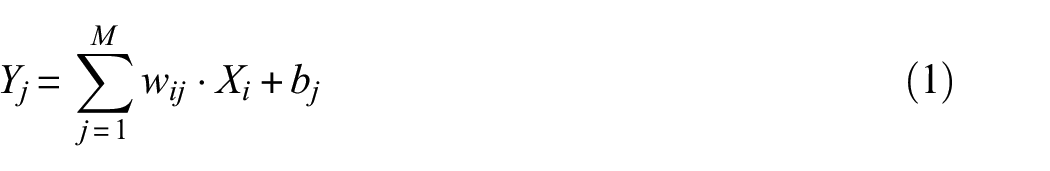
where w_ji is the weight of the connection of ith input to the jth hidden unit, X_i are inputs, b_j is the bias of the jth unit, Y_j is the output of the FNN function, and M is the number of neurons. The activation function associates Y with the output of the node as a = f(Y). Commonly used activation functions are sigmoid, tangent hyperbolic, linear, and Rectified Linear Unit (ReLU).

Figure 1.

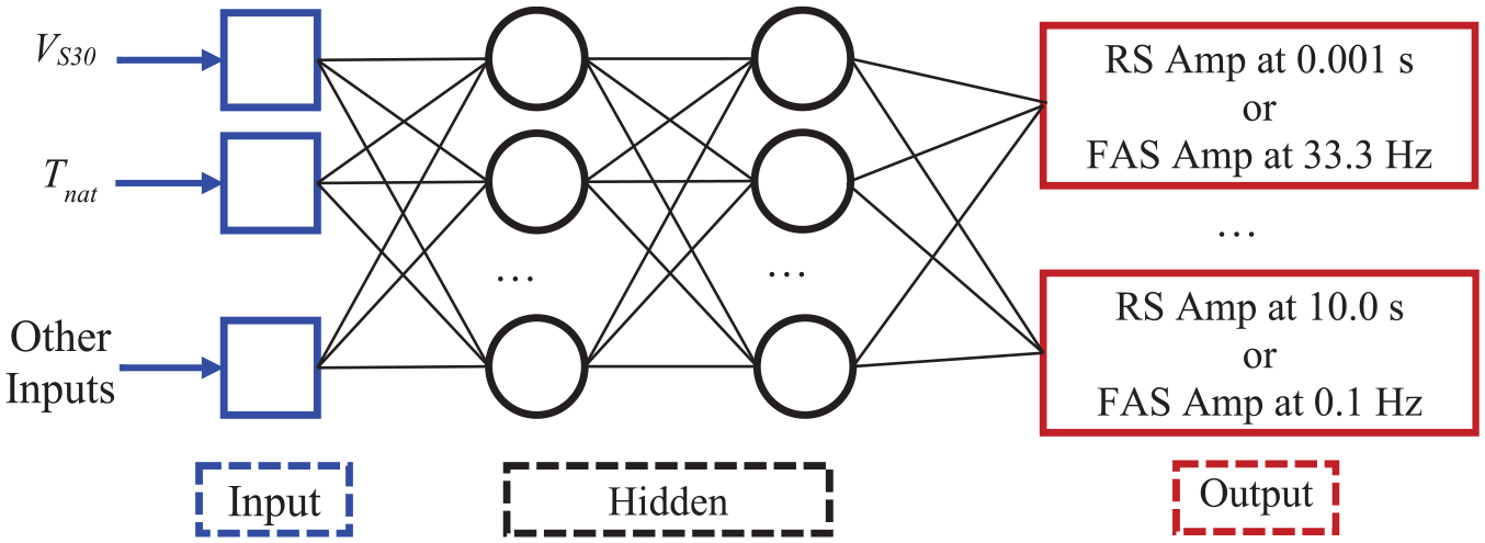
Schematic structure for development of ANN-based RS and FAS amplification models.

This article implements the regression-type multi-layer perceptron (MLP) model (Rumelhart et al., 1986), which is a subset of FNNs and can be regarded as a deep learning FNN. This classification is consistent with the definition provided by LeCun et al. (2015), which states that an ANN model with two hidden layers qualifies as deep. The MLP approach involves (1) executing the FNN and activation functions in a directed graph structure, and (2) updating the weights and biases to reduce the errors computed as the difference between the ANN output and target values. This process is implemented through input, hidden, and output layers of MLP as follows:

Calculation of the FNN function using Equation 1 in each neuron within the hidden layer using the information from the input layer.

Nonlinear mapping of FNN function by the selected activation function of each neuron in the hidden layer.

Error calculation between target values and estimations from the output layer using the loss function.

Updating of weights and biases using an iterative nonlinear optimization algorithm.

All these steps are iterated a given number of times (called an epoch) on input data divided into discrete batches. Batch size is usually selected considering the available computer memory and the targeted level of model accuracy. The loss function and optimization algorithm are selected to minimize the error, which critically affects ANN performance. There are several loss relationships for machine learning techniques (Janocha and Czarnecki, 2017), but two of them, LR₁, which is the sum of the difference between target data and output, and LR₂, which is the sum of the squares of difference between target data and output, are most frequently adopted.

The use of ANN methodologies in earthquake engineering has been investigated by a number of researchers. Derras et al. (2012) developed an ANN-based GMM to predict peak ground acceleration (PGA) using a KiK-net database (kyoshin.bosai.go.jp). ANNs were shown to produce comparable and slightly lower model standard deviations of residuals relative to conventional GMMs using fitted equations (Cotton et al., 2008; Kanno et al., 2006; Zhao et al., 2006). Derras et al. (2014) extended their ANN GMMs to estimate PGA, peak ground velocity (PGV), and 5%-damped pseudo-spectral acceleration (PSA) from 0.01 to 4.0 s. As before, the ANN-based GMMs produced smaller dispersions than conventional GMMs, which are proposed in Akkar and Cagnan (2010) and Bindi et al. (2011). Khosravikia et al. (2019) proposed an ANN-based GMM using a database consisting of strong ground motion data from seismic events in Texas, Oklahoma, and Kansas, an area that experiences frequent anthroprogenic earthquakes (Petersen et al., 2016). Gullu and Ercelebi (2007) utilized three sets of ground motion data from Turkey with 210, 47, and 221 samples to develop a ANN-based approach for PGA prediction. Roten and Olsen (2021) produced ANN models to predict surface-to-downhole site amplification using 600 KiK-net vertical array sites. In their study, 90% of the sites were used to train the models and the remaining 10% were adopted for testing. The ANN yielded a 25% decrease in the mean squared log error between estimations and observed data for the testing data relative to observations and theoretical 1D amplification, which are exposed to known issues with model error in the application of 1D analyses (Bahrampouri et al., 2023; Stewart and Afshari, 2021).

Prior ANN models for site amplification corresponding to a regression-based FNN with MLP structure were also presented by Ilhan et al. (2019), which were trained using limited sampling of site conditions as compared to that proposed in IEA24, and thus, are considered to be relatively outdated models compared to ANNs presented herein. Among the improvements in the present work are the use of a larger simulation dataset for model training and the derivation of models for the standard deviation of residuals.

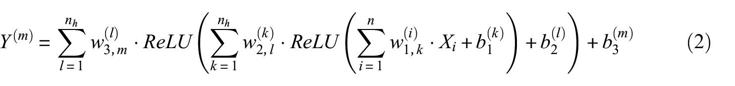
In this article, we explore the use of ANN for RS and FAS ln(amplification) and derive standard deviation relationships from ANN models’ residuals. The functional form to estimate the simulated linear, nonlinear, and total RS and FAS amplification, is presented in Equation 2:

Y^{(m)} = \sum_{l = 1}^{n_{h}} w_{3, m}^{(l)} \cdot ReLU (\sum_{k = 1}^{n_{h}} w_{2, l}^{(k)} \cdot ReLU (\sum_{i = 1}^{n} w_{1, k}^{(i)} \cdot X_{i} + b_{1}^{(k)}) + b_{2}^{(l)}) + b_{3}^{(m)}

(2)

where,

Y ^(m) is the output intensity measure (e.g. RS or FAS ln(amplification) for a given period) for the mth output node.

X₁, X₂, …, X_n are the inputs (V_S30, T_nat, etc.) of ANN-based models. n and n_h represent the number of inputs and the number of nodes in each hidden layer, respectively.

$w_{1, k}^{(i)}$ , $w_{2, l}^{(k)}$ , $w_{3, m}^{(l)}$ are the weights (constants) connecting to the ith input to kth node in first hidden layer, kth node in the first hidden layer to lth node in second hidden layer, and lth node in second layer to mth node in output layer, respectively.

$b_{1}^{(k)}$ , $b_{2}^{(l)}$ , $b_{3}^{(m)}$ are also constants representing the biases for kth node in first hidden layer, lth node in second hidden layer, and mth node in output layer, respectively.

ReLU(x) is the rectified linear unit activation function applied element-wise in first and second hidden layers, defined as ReLU(x) = max(0,x).

ANN-based models derived in this work and their conventional counterparts are constrained to site conditions of V_S30 greater than 200 m/s and motion intensity of PGA at rock (PGA_r) less than 1.0 g. Furthermore, it should be noted that ANNs are differentiable and hence slopes or gradients of the functional forms can be developed as illustrated in Hashash et al. (2004).

RS site amplification models

This study produced a total of six ANN-based models for the amplification of RS ordinates. These include linear models conditioned solely on V_S30 (AL1), the combination of V_S30- and T_nat (AL5), and two complementary (AL9, and AL9-T_p) models (i.e. models built to illustrate the effects of the different input parameters for enhancing model estimates). These models are derived from linear frequency-domain site response analyses as described in IEA24. A nonlinear model (AN2) was derived from differences between nonlinear and linear simulations in which the nonlinear effects are conditioned on V_S30 and the peak acceleration for a reference rock site condition (i.e. PGA relative to V_S = 3000 m/s, denoted PGA_r). Finally, a model for total amplification, including linear and nonlinear effects that are conditioned on V_S30, T_nat, and PGA_r, was developed (denoted AK2). The names of ANNs along with their conventional counterparts are summarized in Table 1, and these labels are determined by adding “A” in front of those of corresponding conventional functions, which were originally presented in Harmon et al. (2019a)—for instance, the V_S30-based ANN and conventional models are named as AL1 and L1, respectively.

Table 1.

List of ANN-based RS and FAS amplification models along with corresponding conventional RS and FAS amplification functions

Inputs	Amplification type	Conventional RS andFAS models^a	ANN RS andFAS models
V_S30	Linear	L1	AL1
V_S30, T_nat	Linear	L5	AL5
V_S30, T_nat, IR,^bΔκ₀^c	Linear	-	AL9^d, AL9-T_p^d
V_S30, PGAr	Nonlinear	N2	AN2
V_S30, T_nat, PGAr	Total	K2	AK2

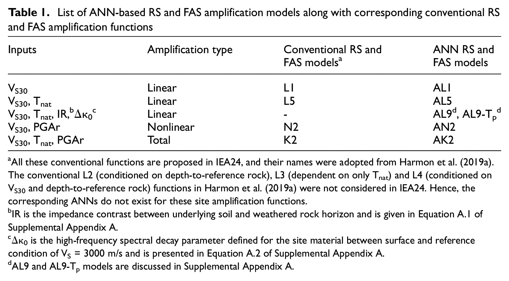
All these conventional functions are proposed in IEA24, and their names were adopted from Harmon et al. (2019a). The conventional L2 (conditioned on depth-to-reference rock), L3 (dependent on only T_nat) and L4 (conditioned on V_S30 and depth-to-reference rock) functions in Harmon et al. (2019a) were not considered in IEA24. Hence, the corresponding ANNs do not exist for these site amplification functions.

IR is the impedance contrast between underlying soil and weathered rock horizon and is given in Equation A.1 of Supplemental Appendix A.

Δκ₀ is the high-frequency spectral decay parameter defined for the site material between surface and reference condition of V_S = 3000 m/s and is presented in Equation A.2 of Supplemental Appendix A.

AL9 and AL9-T_p models are discussed in Supplemental Appendix A.

Model development included training and testing datasets, with an individual value of site amplification referred to as a “sample.” Training samples of site amplifications comprise 90% of the simulations, corresponding to 1,097,050 samples for linear amplification and 999,460 samples for total or nonlinear amplification. Potential bias in the ANN-based models that might arise from including amplification data from the same site in both samples—due to this data partitioning approach (i.e. 90% and 10% of the entire dataset for the training and testing samples, respectively)—is expected to be limited, as elaborated in the subsection titled “Alternative Training and Testing Samples for ANN-based Models” in Supplemental Appendix A. The number of data for the total and nonlinear ANNs is less than for the linear ANNs because nonlinear analyses with maximum strain greater than 1.0% are excluded from the model development as discussed subsequently. The elimination of nonlinear simulations with maximum strain exceeding 1.0% stems from the base-isolation behavior (e.g. Zalachoris and Rathje, 2015) observed in the 1D site response approach as explained in IEA24. Hence, it is highlighted that this threshold is unrelated to the ANN technique and regression methodology. These large training datasets are then randomly sampled into approximately 5000 batches, each comprising 400 simulations, which are then utilized to train the ANNs. This partitioning facilitates the utilization of reduced memory during the weight updating phase of the ANN and accelerates training. The testing samples comprise 10% of the simulations, which are used to test the predictive capability of the ANN-based site amplification models through comparison with corresponding linear (V_S30-based L1 and V_S30- and T_nat-based L5), nonlinear (V_S30- and PGA_r-based N2) and total (V_S30, T_nat and PGA_r-dependent K2) conventional relationships (Table 1) proposed in IEA24 using the same simulated amplification dataset.

Two hidden layers with 200 nodes each are adopted for all models (Figure 1), and the activation function is selected as ReLU. Learning rate, which is defined as the step size at which the model learns (Bishop, 1995), was selected as 0.0001 because it produced the lowest error from the testing dataset, which is also consistent with typical learning rates of 10⁻⁶ to 1.0 (Bengio, 2012). For AL1 (RS and FAS) and other ANNs (i.e. AL5, AL9, AL9-T_p, and AN2), the corresponding selected epochs are 400 and 5000, respectively. The rationale behind the selection of this number of epochs was to adopt the ANN model that successfully encapsulates the distinct features of the amplification data (e.g. peak responses due to sharp impedance contrasts, and reductions of amplification at soft sites at short periods due to cumulative effect of soil damping). Moreover, the Adam optimizer (Kingma and Ba, 2014), which is a stochastic gradient descent method that is well-suited for problems involving large numbers of data points and parameters, is utilized along with LR₂ type loss relationship to define the error between training data and model estimations.

The output layer consists of 125 nodes which produce the estimated RS natural logarithms of amplification, that is, ln(amplification), at 125 periods between oscillator period (T_OSC) of 0.001 and 10.0 s. A linear activation function, which is an identity function for which output is directly proportional to input (Goodfellow, 2016), is assigned to each output node. TensorFlow (Abadi et al., 2016), which can be imported as a library in Python, is utilized for training ANN-based models.

Linear amplification

Figure 2a and b compares the L1 estimations from IEA24 and the ANN-based AL1 model for T_OSC = 0.1 and 1.0 s, both of which are based solely on V_S30. Although these models exhibit analogous behavior for T_OSC of 1.0 s (Figure 2b), AL1 better captures the binned means of RS amplification (e.g. the peak, which is observed at V_S30∼ 900 m/s for T_OSC of 0.1 s) and results from a strong impedance contrast at shallow sites (e.g. depth of overburden soil to hard rock (V_S reference of 3000 m/s) of <30.0 m). This is also reflected by the mean residuals aligning with zero, as shown in Figure 2c. It should be noted that this peak feature in the simulated amplification data used to train the ANNs is not represented in empirically derived amplification models (Parker et al., 2019; Stewart et al., 2020). Hence, while the ANN models better capture this attribute of the simulated data, which is associated with 1D site response assumption, it remains an open question whether both ANNs and conventional functions better represent amplification as observed under field conditions.

Figure 2.

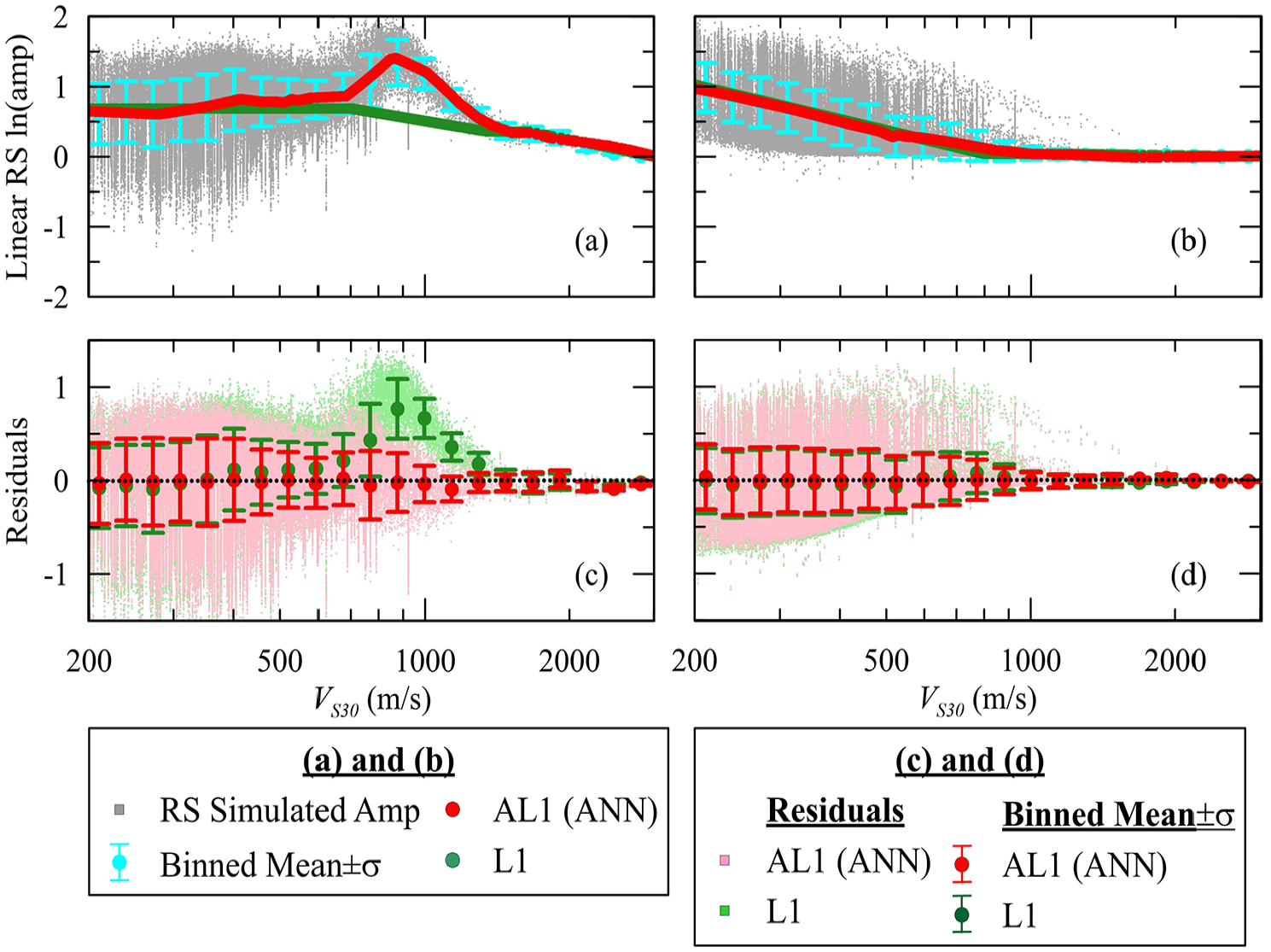
Comparison of model predictions from L1 and ANN-based AL1 (V_S30-based) along with linear RS ln(amp) and its binned mean ±1σ for T_OSC of (a) 0.1 s and (b) 1.0 s. The residuals of L1 and AL1 models are given for T_OSC of (c) 0.1 s, (d) 1.0 s (testing dataset).

The T_nat effects on linear RS amplification are modeled through ANN-based model AL5, which utilizes the T_nat of randomized profiles in addition to their V_S30 values, adopted for training AL1, and is the counterpart of L5 (V_S30 and T_nat) in IEA24. Figure 3 presents the performance of the ANN-based AL5 model along with the corresponding L5 conventional function. Unlike Figure 2, the amplification models in Figure 3 do not appear as lines due to the inclusion of varying T_nat values for sites with identical V_S30s (i.e. sites with same V_S30s but with different depth-to-reference condition values) as inputs in the ANN estimations. Two main changes are observed: (1) for T_OSC = 0.1 s, AL5 more successfully captures the location and amplitude of peak amplification at V_S30∼ 950 m/s along with the decay of amplification at low V_S30 values, which produces mean residuals at V_S30∼ 950 m/s that are close to zero, relative to L5 and (2) again for T_OSC = 0.1 s, AL5 produces less scattered residuals relative to those of L5 for V_S30 > 950 m/s. The enhancements in amplification estimations provided by AL5 as compared to AL1 (i.e. the influence of incorporating T_nat in model inputs on ANN’s performance) are further discussed in “Models’ standard deviation” section.

Figure 3.

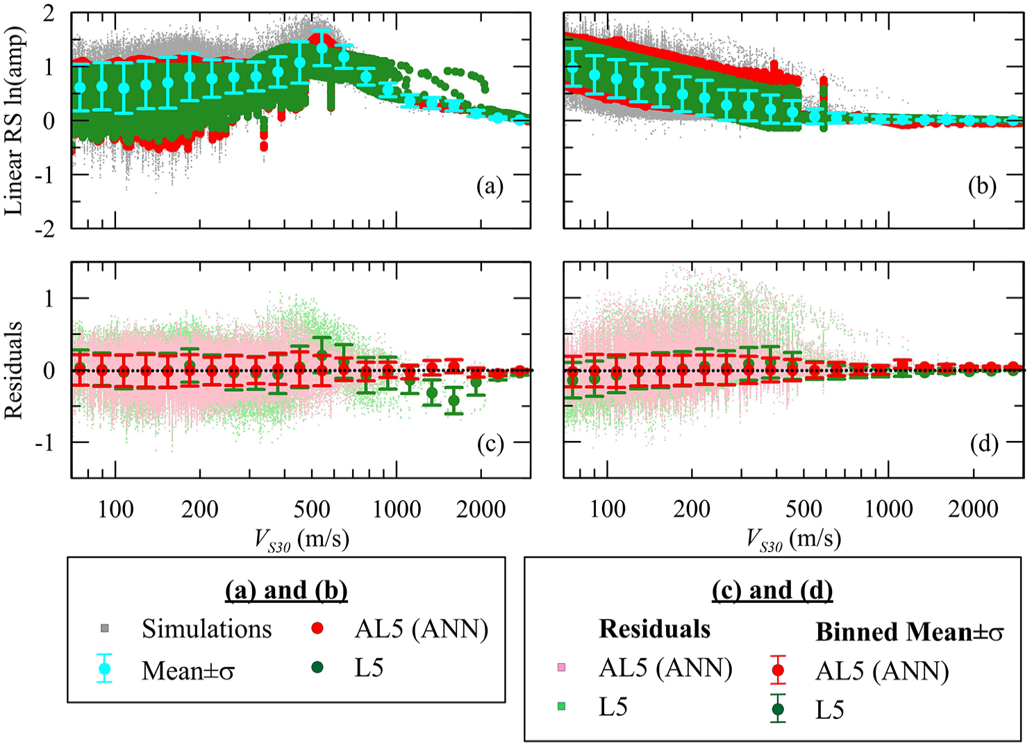
Comparison of model predictions from L5 and ANN-based AL5 using the same V_S30 and T_nat inputs along with linear RS ln(amplification) and binned mean of ln(amplification) ±1σ for T_OSC of(a) 0.1 s and (c) 1.0 s. The models’ residuals with their binned mean ±1σ are given for T_OSC of(c) 0.1 s and (d) 1.0 s (testing dataset).

Nonlinear and total amplification

The nonlinear (NL) RS amplification model accounts for amplification differences between NL and linear (L) analyses. Figure 4 demonstrates the nonlinear amplification data binned as functions of V_S30 and PGA_r, for the AN2 and N2 models for relatively short (0.3 s) and long (1.0 s) T_OSC, respectively. AN2 is found to yield similar mean estimations of nonlinear amplification to N2. The jaggedness in AN2 estimations (e.g. the line representing the nonlinear amplification at V_S30 conditions of 270 m/s and 0.4 g < PGA_r < 0.6 g) is more pronounced than the jaggedness in nonlinear amplification, which occurs due to the gaps in these datasets resulting from the exclusion of nonlinear simulations with maximum strain values exceeding 1.0% from the training and testing databases. Because the ANN technique adjusts its coefficients to learn the data trends, the jaggedness in the AN2 model estimations should be attributed to the inherent data behavior rather than to a deficiency in ANN’s equational form (Equation 2). If future implementations of AN2 are pursued (e.g. the integration of AN2 with GMMs in probabilistic seismic hazard applications), (1) re-training AN2 through training samples without excluding the simulations with maximum strain greater than 1.0, or (2) smoothing techniques may be considered to avoid pronounced jaggedness in AN2. However, this is beyond the scope of this article. Moreover, AN2 captures an increase in nonlinear amplification under conditions of high V_S30 (≥650 m/s) and large PGA_r values (≥0.4 g) for short periods (0.3 s). This behavior arises because the amplification from nonlinear analysis exceeds the corresponding linear amplification (i.e. that obtained from a linear analysis using the same site and motion combination) as a consequence of period elongation. Finally, this behavior cannot be modeled by the N2 model of IEA24, as the f₂ coefficients—representing the nonlinear behavior in terms of the rate of change of site amplification with the intensity of the input motion—are constrained to be negative.

Figure 4.

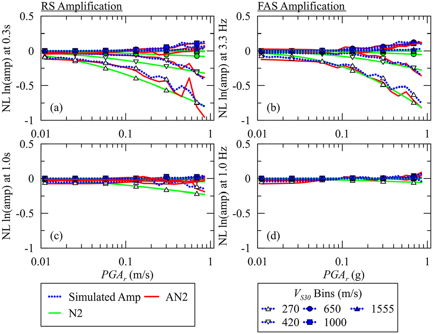
Model predictions from N2 and ANN-based AN2 for RS (a, c) and FAS (b, d) for nonlinear site amplification along with corresponding simulated amplification data as functions of V_S30 and PGA_rfor T_OSC of 0.3 and 1.0 s, and frequency of 3.3 and 1.0 Hz, respectively.

Figure 5 presents total amplifications for T_OSC of 0.1 and 1.0 s for the conventional model (K2) and ANN-based model (AK2) trained using NL simulation results. Although the linear part of the K2 model includes an f(T_nat) component, its performance misses the peak amplification at V_S30∼ 1000 m/s for T_OSC of 0.1 s (i.e. the mean of K2’s residuals at V_S30∼ 1000 m/s is above 0 as seen in Figure 5c). These non-zero residuals are absent in the AK2 model, which is similar to the AL5 model performance.

Figure 5.

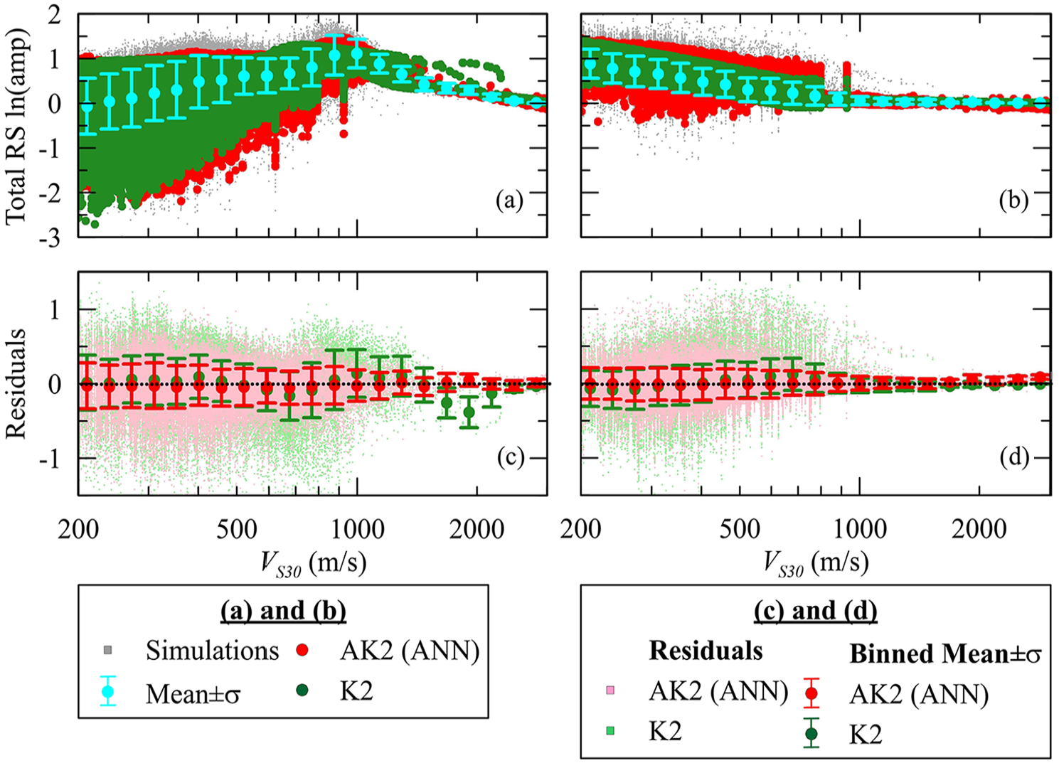
Comparison of model predictions from K2 (V_S30, T_nat, PGA_r) and ANN-based AT5 (V_S30, T_nat, and PGA_r) along with total RS ln(amplification) from nonlinear simulations and its binned mean ±1σ for T_OSC of (a) 0.1 s, (b) 1.0 s. The models’ residuals are presented for T_OSC of (c) 0.1 s and (d) 1.0 s (testing dataset).

FAS amplification

ANN-based FAS models utilize the same structure as the RS models except the output layer consists of 110 nodes providing FAS ln(amplification) for frequencies between 0.1 and 33.3 Hz (i.e. FAS ln(amplification) at 110 frequencies between 0.1 and 33.3 Hz). As before, the samples corresponding to 90% of the simulated amplifications (i.e. 1,097,050 simulations for linear FAS amplification, which correspond to site transfer functions (Kramer and Stewart, 2025), and 999,460 simulations for total or nonlinear FAS amplification) were used to train the ANN-based FAS models and the remaining 10% of the simulations were used for testing the predictions of FAS amplification. Figure 6 compares the performance of the L5 model (conditioned on V_S30 and site natural frequency, f_nat) and the ANN-based AL5 model for linear FAS amplification for frequencies of 10.0 and 1.0 Hz. As with Figure 3, the models do not manifest as lines in Figure 6 owing to the incorporation of different f_nat values for sites with identical V_S30s as inputs to the ANN estimations. Figure 6c and d, show non-zero binned means of L5 (FAS) residuals but nearly zero residuals for AL5 (FAS), which is similar to the linear RS results. Similar outcomes were obtained for the V_S30-dependent AL1 models (Supplemental Figure A.1).

Figure 6.

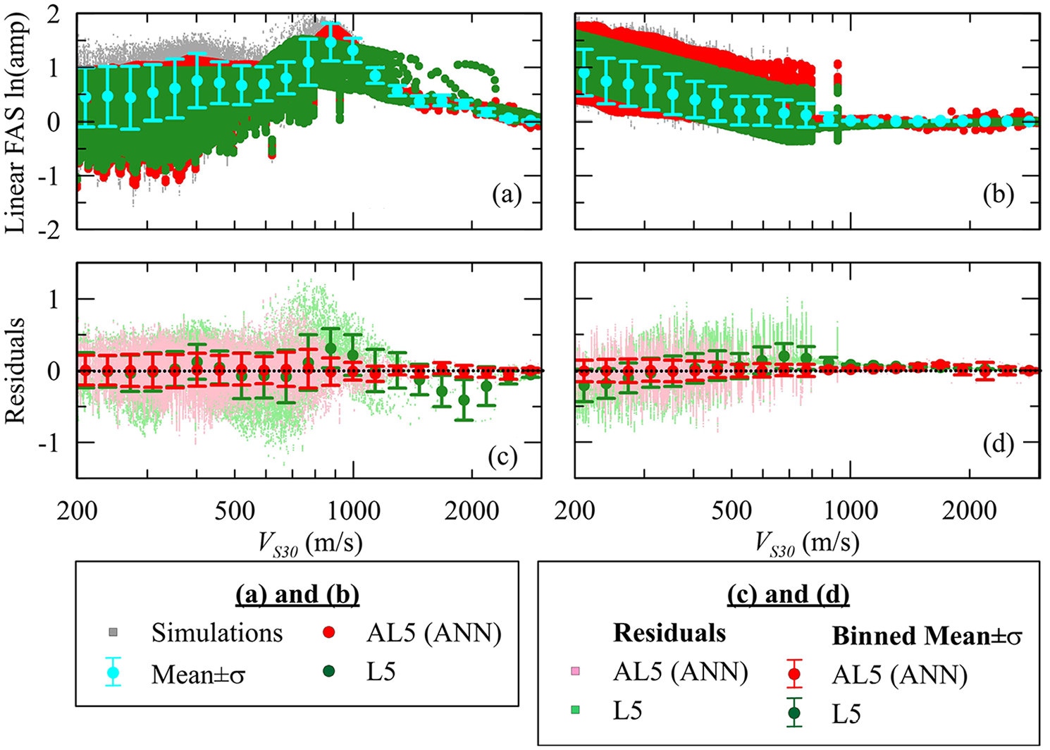
Comparison of model predictions from L5 (V_S30 and f_nat) and ANN-based AL5 (V_S30 and f_nat) along with linear FAS ln(amp) and its binned mean ±1σ for frequency of (a) 10.0 Hz and (b) 1.0 Hz. Models’ residuals are presented for frequency (f) of (c) 10.0 Hz and (d) 1.0 Hz (testing dataset).

Nonlinear and total FAS models are presented in a similar manner to the RS models in Figure 4b and d, and Supplemental Figure A.2, respectively. The mean AN2 (FAS) model behaves similarly to the N2 model but the total ANN model (AK2) residuals’ dispersions are lower (Supplemental Figure A.2) relative to conventional K2. It is possible to extend ANN models (Equation 2) to include other input parameters that might be hypothesized as affecting predicted site amplification (e.g. high-frequency spectral decay (Δκ₀), impedance ratio (IR) between overlying sediment and weathered rock or reference condition of V_S = 3000 m/s, and predominant period (T_p) parameter). The extension of the current models to include additional input parameters is discussed in Supplemental Appendix A.

Models’ standard deviation

The standard deviation (σ) of a model is computed from the residuals defined as the difference between the natural logs of site amplification values from simulations and model predictions in natural log units. These σ values include both motion-to-motion and site-to-site variability, which are provided for conventional amplification functions by IEA24. Figure 7 shows the AL1 and AL5 dispersion terms for both the RS and FAS amplifications along with a model fit (σ_Flin) that matches the form selected by IEA24. There is a reduction in σ_Flin for AL5 in Figure 7c for V_S30 values exceeding approximately 800 m/s. This decrease is also evident in the σ of linear site amplification at these sites (i.e. in the error bars of the binned mean of linear amplification for V_S30 ≥ ∼800 m/s in Figure 6). This condition is anticipated, as the impedance contrast in stiffer sites is less pronounced than in profiles with lower V_S30 values, resulting in a lower σ for stiffer sites compared to softer sites. The corresponding coefficients for the σ_Flin model are depicted in Supplemental Figures A.5 to A.8. In a similar manner, σ_Fnl models were derived using the same functional forms from IEA24 for AN2 RS and FAS.

Figure 7.

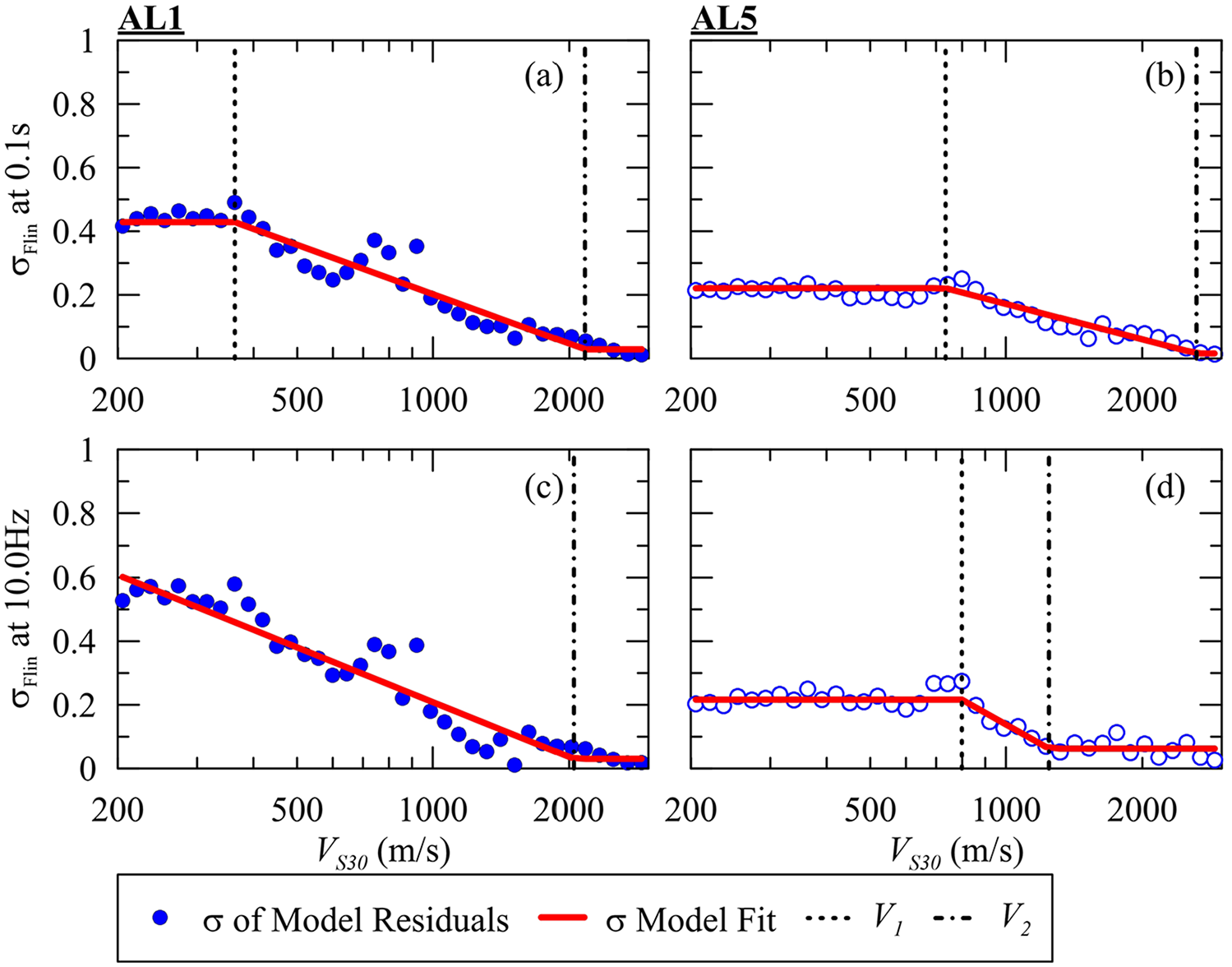
Standard deviations of residuals for evenly distributed log(V_S30) bins for T_OSC of 0.1 s and 10 Hz and models fitted to results (red lines). AL1 RS (a) and FAS (c) and AL5 RS (b) and FAS (d).

Figure 8 compares standard deviations from the ANN and conventional models. For the σ_Flin and σ_FS of RS models, considerable levels of reductions up to 12%−18% for linear (AL1, AL5) and The σ for total amplification models (σ_FS) can be computed by taking into account that the σ_Flin and σ_Fnl showed near-zero correlation in IEA24, and thus they are independent:

σ_{FS} = \sqrt{σ_{Flin}^{2} + σ_{Fnl}^{2}}

(3)

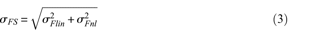
where σ_Flin is from AL1 or AL5 and σ_Fnl is from AN2.

Figure 8.

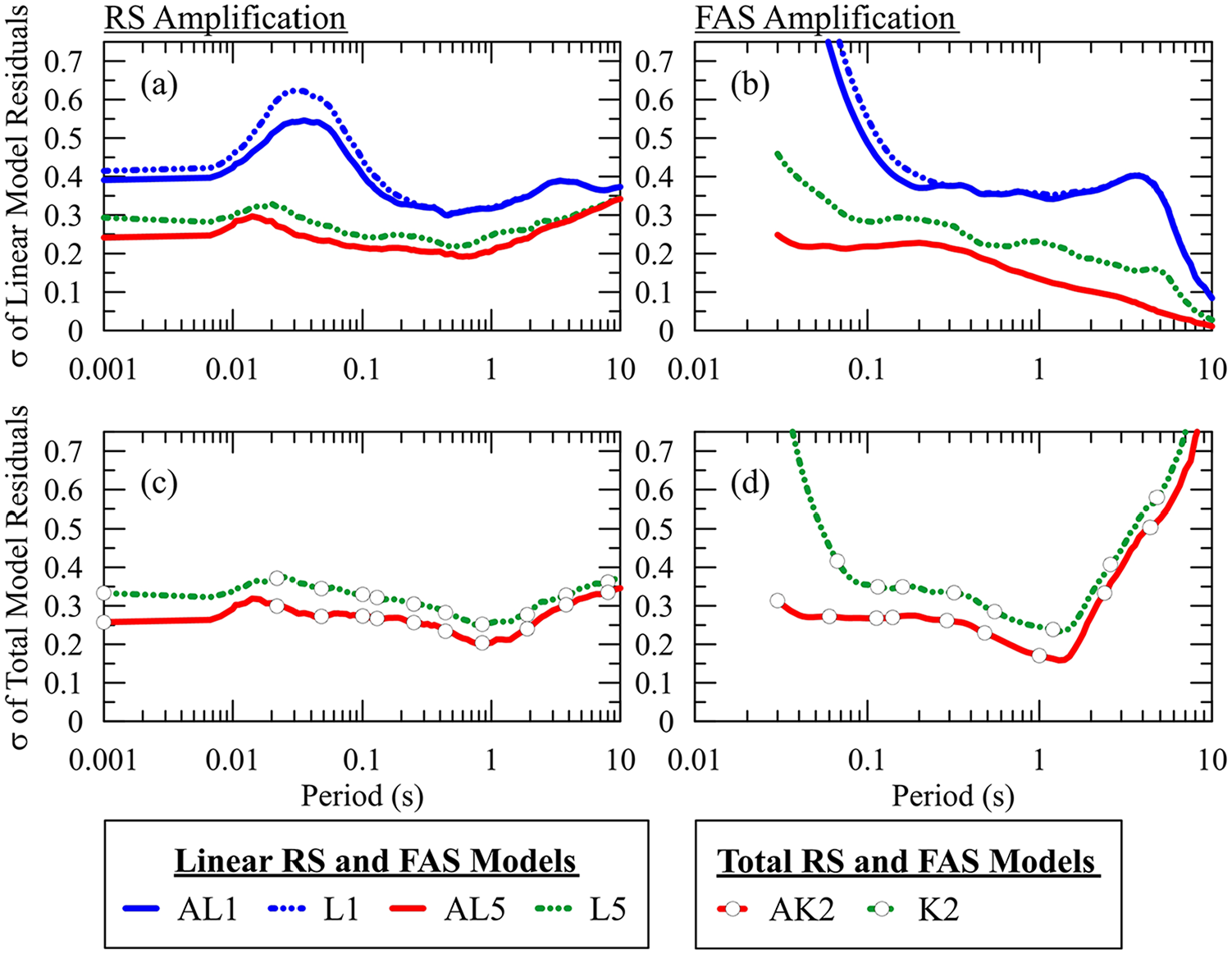
Standard deviation (σ) of residuals of linear conventional L1 and L5, and ANN-based AL1 and AL5 RS (a) and FAS (b) models, and total conventional K2, and ANN-based AT5 RS (c) and FAS (d) models (testing dataset).

23% for total amplification models (AK2), respectively, are achieved compared to their conventional counterparts. FAS models have higher σ values in AL1 and L1 at short periods due to limitations in the ability of V_S30-based models to capture the substantial reduction in simulated FAS ln(amplification) for soft and deep sites due to cumulative damping effects. These effects are less evident in RS data because single-degree-of-freedom oscillator responses approach PGA at short periods (e.g. Bora et al., 2016). The inclusion of the f_nat term in AL5 or L5 (i.e. employing both V_S30 and f_nat) mitigates this issue, resulting in significantly lower σ_Flin compared to AL1 or L1. Maximum decreases of σ_FS by AL1, AL5, and AK2 as compared to their conventional counterparts are 15.7%, 70.8%, and 67.2%, respectively. Similar evaluations of σ_Flin and σ_FS from the ANN-based and conventional models via testing samples (Supplemental Figure A.10) were found to yield analogous results to σ_Flin and σ_FS assessed using the training dataset.

Shallow profile response

The behavior of shallow profiles, which are defined as the sites with overburden soil depths to reference rock (Z_Soil) < 30 m, based on the shallow site definition in Nikolaou et al. (2001), deviates from the median site response from the overall database due to a preponderance of short period resonances. Nikolaou et al. (2001) evaluated this phenomenon through comparisons of surface RS from EL analyses using a profile with V_S30 = 220 m/s and Z_Soil = 15.0 m with a design spectrum from New York City Department of Transportation (NYCDOT, 1998). These comparisons demonstrated that computed RS exceeds the NYCDOT (1998) specta for T_OSC ≤ ∼ 0.4 s. Motivated by this disparity, the performance of conventional and ANN models for shallow sites is investigated.

Figure 9a and b shows linear RS and FAS amplification, respectively, for the training samples corresponding to all and shallow sites (Z_Soil < 30.0 m). The results show that shallow sites have higher amplifications than the full dataset for short periods of 0.1 s and V_S30 ≤ 400 m/s. The AL5 model better represents the location and height of the peak shallow amplification around V_S30 = 950 m/s than the L5 model (Figure 9c and d). Improved performance of AL5 relative to L5 is also evident from residuals (Figure 9e and f). Similar results for models AK2 and K2 are presented in Supplemental Figure A.9.

Figure 9.

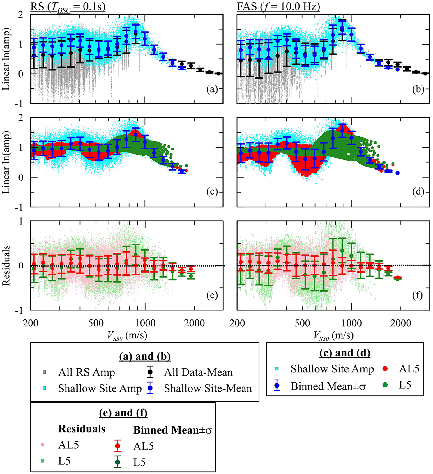
Comparison of amplifications derived for full dataset and subset for shallow sites. Results are shown for the specific conditions of T_OSC = 0.1 s for RS and 10 Hz for FAS. (a) and (b) simulated amplifications; (c) and (d) model predictions (L5 and AL5); (e) and (f) model residuals.

Example applications to selected CENA sites

To demonstrate the implementation and performance of the conventional functions from IEA24 and the ANN-based models in this article, their predictions are compared to results of site-specific response analyses for two profiles (one from New York City (NYC) presented in Nikolaou et al. (2001) and the other from Pecos, Texas [TX] in Li et al. (2020)). The ANN models are applied using the Excel spreadsheet implementation in Supplemental Appendix B. The NYC and TX profiles were not in the training data sets for ANN model development. All analyses are 1D and include L and NL representations of material behavior. For these simulations:

Three rock outcrop motions (PGA of 0.1, 0.3, 0.51 g) from the Harmon et al. (2019b) database are selected.

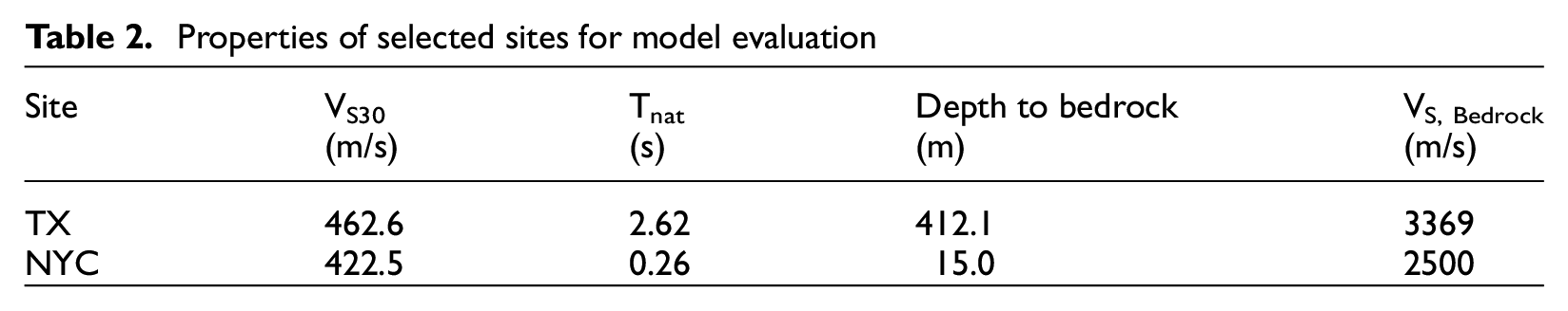
The V_S profiles and profile properties of NYC and TX sites are given in Figure 10 and Table 2, respectively. These profiles possess similar V_S30 values but different T_nat values. Figure 11 highlights that both NYC and TX profiles are within V_S30 and T_nat parametric range contained in the training samples. The reference condition for the NYC and TX sites are V_S = 2500 and 3000 m/s, respectively.

The stratigraphy of the NYC site is composed of (1) two sand layers between 0.0−5.0 and 8.2−11.3 m, (2) a clay layer sandwiched between these two sand layers, and (3) a gravel layer with a thickness of 3.7 m underlying this sediment. The unit weight and OCR (overconsolidation ratio) exist for each material and clay stratum, respectively. The friction angle (ϕ) values of cohesive and cohesionless soils were set as 30° and 32° as detailed in Hashash et al. (2021). The ϕ parameter was utilized to compute (1) the lateral earth-pressure coefficients at rest (K₀) for reference MRD (modulus reduction and damping) curves from Darendeli (2001), and (2) the strength input for the GQ/H model (Groholski et al., 2016), which was fit to reference MRD curves.

D_min values are estimated using the Campbell (2009) Q-V_S Model 1.

Figure 10.

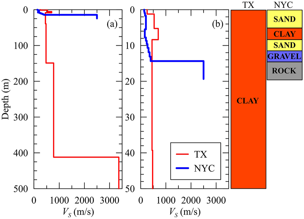
V_S profiles of Pecos, TX, and New York City to the depth of (a) 500 m and (b) 50.0 m. The stratigraphic profiles reflect the depth axis in figure (b).

Table 2.

Properties of selected sites for model evaluation

Site	V_S30(m/s)	T_nat(s)	Depth to bedrock(m)	V_{S, Bedrock}(m/s)
TX	462.6	2.62	412.1	3369
NYC	422.5	0.26	15.0	2500

Figure 11.

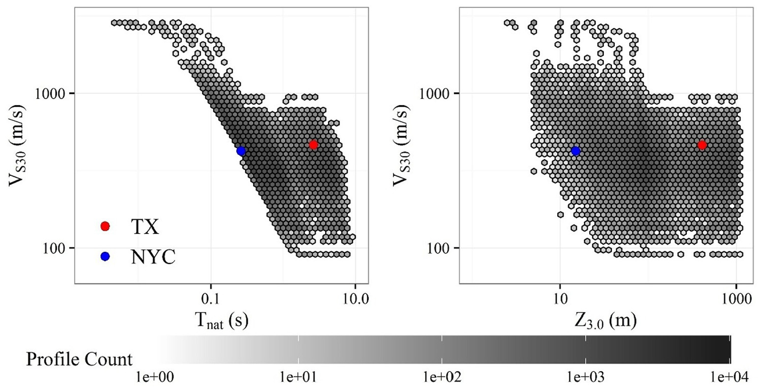
Density plots of IEA24 database in (a) V_S30-T_nat and (b) V_S30-Z_3.0 (depth to V_S = 3000 m/s) spaces.

Figure 12 compares for the NYC site the linear amplification from 1D L analysis using the three input motions; the mean of the simulated linear amplifications are shown along with predictions of the amplification from the L5 and AL5 models, which are shown as the mean ± σ_Flin. The site-specific results have strong resonance effects that produce a peak around T_OSC = 0.2 s; this peak is underestimated by the mean L5 model, being close to L5 + σ_Flin. The location and level of this resonant peak are better captured by AL5 along with a better representation of the trough between the first and second mode peaks (0.075 s < T_OSC < 0.2 s). Figure 13 presents similar results for NL simulations, where the site-specific total amplifications are compared to AK2 and K2 predictions. In this case, the first mode peak occurs at T_OSC≈ 0.3 s (about 50% lengthened relative to the L solution) for the PGA_r = 0.1 g input motion and it progressively shifts to longer periods as PGA_r increases. This behavior is not captured by the K2 model, which does not allow for period elongation, but is better represented by the AK2 model because the ANN adjusts to be consistent with the simulated nonlinear response.

Figure 12.

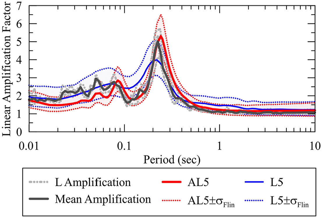
(NYC site) comparison of linear site-specific amplification and ergodic ANN-based AL5 and conventional linear L5 site amplification models with ±1 standard deviation (σ_Flin).

Figure 13.

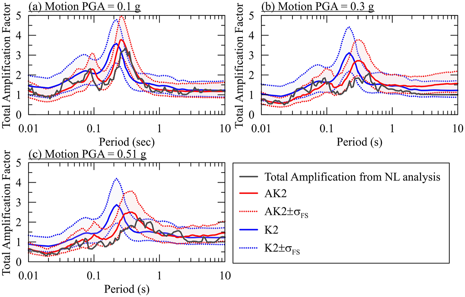
(NYC site) comparison of total site-specific amplification computed for PGA_r of (a) 0.1 g, (b) 0.3 g and (c) 0.51 g and ergodic ANN-based AK2 and conventional total K2 site amplification models with ±1 standard deviation (σ_FS).

Figures 14 and 15 present similar results for the deeper TX site. As shown in Figure 15, both conventional and ANN-based models seem to envelope site-specific amplifications from NL analyses for T_OSC ≤ ∼ 0.8 s. The ANN model more accurately captures the location of the peak linear amplification (Figure 14) along with the period elongation under nonlinear conditions (Figure 15). However, the first mode linear and total amplification peaks are underestimated by the AL5 and AK2 ANN models and by the L5 and K2 conventional models, respectively. Even though TX site falls within V_S30-PGA_r distribution of training samples, such deviations of model estimations from computed site-specific peak amplification are expected since no model can be expected to perfectly fit the amplification for an individual site.

Figure 14.

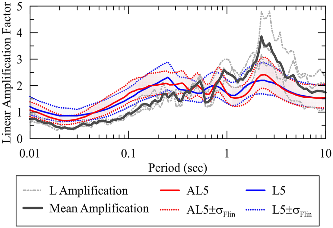
(TX site) comparison of linear site-specific amplification and ergodic ANN-based AL5 and conventional linear L5 site amplification models with ±1 standard deviation (σ_Flin).

Figure 15.

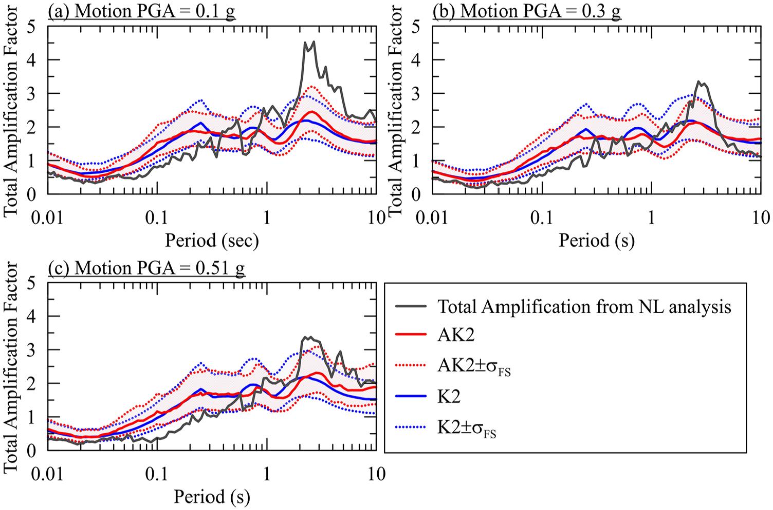
(TX site) comparison of total site-specific amplification computed for PGAr values of(a) 0.1 g, (b) 0.3 g and (c) 0.51 g and ergodic ANN-based AK2 and conventional total K2 site amplification models with ±1 standard deviation (σ_FS).

Recommendations and conclusions

This article presents a series of ANN-based linear, nonlinear, and total (linear plus nonlinear) RS and FAS site amplification models for a reference velocity condition of V_S = 3000 m/s for sites in CENA highlighting the promise of ANN’s use as site amplification models. These models are developed using a database comprising 3.6 million 1D simulations from Ilhan et al. (2024). The performance of ANNs is evaluated through comparison with their conventional regression model counterparts, yielding that:

ANNs successfully reduced residuals and the standard deviation (σ) of model estimations, with reductions of up to 23.0% for RS and 70.8% for FAS compared to commonly used amplification functions.

ANNs can capture simulated site-specific response characteristics: (1) the location and amplitude of the first-mode simulated amplification, (2) the simulated shallow site amplification, and (3) the period elongation behavior (i.e. the shift in the period of peak amplification to longer period values) as a consequence of soil nonlinearity, which cannot be modeled by conventional site amplification functions.

The conventional and ANN-based models are subject to the limitations of the simulation dataset on which they are based. This includes the constraints of 1D site response theory, such as the absence of basin effects. The applicability of models is restricted to sites with V_S30 > 200 m/s and PGA_r less than 1.0 g to avoid base-isolation behavior during 1D simulations that can result in unrealistically high strains. The equations that are fit when training ANN models (e.g. Equation 2) are learned directly from the data rather than being proposed as a priori forms in conventional functions, and as a result they are unlikely to extrapolate well beyond the limits of the training data. These limits include lower or higher V_S30 values, higher PGA_r values, and profile characteristics that are not contained in the training set. To facilitate the use of the ANN-based models, an Excel spreadsheet is provided as an appendix so that researchers can explore these models in their own applications.

In this article, we do not explore how to deploy ANN’s site amplification models in seismic hazard analysis or in combination of commonly used GMMs. This is beyond the scope of this work but is an important effort to undertake in the future.

Supplemental Material

sj-docx-1-eqs-10.1177_87552930251343630 – Supplemental material for Artificial neural network−based simulated site amplification models for Central and Eastern North America

Supplemental material, sj-docx-1-eqs-10.1177_87552930251343630 for Artificial neural network−based simulated site amplification models for Central and Eastern North America by Okan Ilhan, Youssef MA Hashash, Jonathan P Stewart, Ellen M Rathje, Sissy Nikolaou and Kenneth W Campbell in Earthquake Spectra

Supplemental Material

sj-xlsx-2-eqs-10.1177_87552930251343630 – Supplemental material for Artificial neural network−based simulated site amplification models for Central and Eastern North America

Supplemental material, sj-xlsx-2-eqs-10.1177_87552930251343630 for Artificial neural network−based simulated site amplification models for Central and Eastern North America by Okan Ilhan, Youssef MA Hashash, Jonathan P Stewart, Ellen M Rathje, Sissy Nikolaou and Kenneth W Campbell in Earthquake Spectra

Footnotes

Declaration of conflicting interests

The author(s) declared no potential conflicts of interest with respect to the research, authorship, and/or publication of this article.

Funding

The author(s) received no financial support for the research, authorship, and/or publication of this article.

Disclaimers

Certain trade names or company products are mentioned in the text to specify adequately the analytical procedures used. In no case does such identification imply recommendation or endorsement by the National Institute of Standards and Technology (NIST), nor does it imply that the products are the best available for the purpose. In this document, we have provided link(s) to website(s) that may have information of interest to our users. NIST does not necessarily endorse the views expressed or the facts presented on these sites. Furthermore, NIST does not endorse any commercial products that may be advertised or available on these sites.

ORCID iDs

Okan Ilhan

Jonathan P Stewart

Data and resources

The coefficients (i.e. weights and biases) of all proposed ANN-based models are presented in Excel file submitted as Appendix B. The same file includes spreadsheets that allow the readers to calculate and visualize the ANN-based model estimations for the given inputs. The spreadsheet titled “INTRODUCTION” in this Excel file B elaborates on the content of Appendix-B.

Supplemental material

Supplemental material for this article is available online.

References

Abadi

Barham

Chen

Davis

Dean

Devin

Ghemawat

Irving

Isard

Kudlur

Levenberg

Monga

Moore

Murray

Steiner

Tucker

Vasudevan

Warden

Wicke

Zheng

(2016) TensorFlow: A system for large-scale machine learning. In: 12th (USENIX) symposium on operating systems design and implementation (OSDI 16), Savannah, GA, 2–4 November, pp. 265–283. Berkeley, CA: USENIX Association.

Abrahamson

Youngs

(1992) A stable algorithm for regression analyses using the random effects model. Bulletin of the Seismological Society of America 82(1): 505–510.

Akkar

Çağnan

(2010) A local ground-motion predictive model for Turkey, and its comparison with other regional and global ground-motion models. Bulletin of the Seismological Society of America 100(6): 2978–2995.

Bahrampouri

Rodriguez-Marek

(2023) One-dimensional site response analysis: Model error estimation. Bulletin of the Seismological Society of America 113(1): 401–416.

Bengio

(2012) Practical recommendations for gradient-based training of deep architectures. In: Neural networks: Tricks of the trade, 2nd ed (pp. 437–478). Berlin, Heidelberg: Springer Berlin Heidelberg.

Bindi

Pacor

Luzi

Puglia

Massa

Ameri

Paolucci

(2011) Ground motion prediction equations derived from the Italian strong motion database. Bulletin of Earthquake Engineering 9: 1899–1920.

Bishop

(1995) Neural Networks for Pattern Recognition. Oxford: Oxford University Press.

Bora

Scherbaum

Kuehn

Stafford

(2016) On the relationship between Fourier and response spectra: Implications for the adjustment of empirical ground-motion prediction equations (GMPEs). Bulletin of the Seismological Society of America 106(3): 1235–1253.

Brillinger

Preisler

(1985) Further analysis of the Joyner-Boore attenuation data. Bulletin of the Seismological Society of America 75(2): 611–614.

10.

Campbell

(2009) Estimates of shear-wave Q and k 0 for unconsolidated and semiconsolidated sediments in Eastern North America. Bulletin of the Seismological Society of America 99(4): 2365–2392.

11.

Cotton

Pousse

Bonilla

Scherbaum

(2008) On the discrepancy of recent European ground-motion observations and predictions from empirical models: Analysis of KiK-net accelerometric data and point-sources stochastic simulations. Bulletin Seismological Society of America 98: 2244–2261.

12.

Darendeli

(2001) Development of a new family of normalized modulus reduction and material damping curves. The University of Texas at Austin.

13.

Derras

Bard

Cotton

(2014) Towards fully data driven ground-motion prediction models for Europe. Bulletin of Earthquake Engineering 12(1): 495–516.

14.

Derras

Bard

Cotton

Bekkouche

(2012) Adapting the neural network approach to PGA prediction: An example based on the KiK-net data. Bulletin of the Seismological Society of America 102(4): 1446–1461.

15.

Goodfellow

(2016) Deep Learning. Cambridge, MA: MIT Press.

16.

Groholski

Hashash

Kim

Musgrove

Harmon

Stewart

(2016) Simplified model for small-strain nonlinearity and strength in 1D seismic site response analysis. Journal of Geotechnical and Geoenvironmental Engineering 142(9): 04016042.

17.

Güllü

Erçelebi

(2007) A neural network approach for attenuation relationships: An application using strong ground motion data from Turkey. Engineering Geology 93(3–4): 65–81.

18.

Harmon

Hashash

YMA

Stewart

Rathje

Campbell

Silva

Ilhan

(2019a) Site amplification functions for Central and Eastern North America-part II: Modular simulation-based models. Earthquake Spectra 35: 815–847.

19.

Harmon

Hashash

YMA

Stewart

Rathje

Campbell

Silva

Musgrove

Ilhan

(2019b) Site amplification functions for Central and Eastern North America-part I: Simulation dataset development. Earthquake Spectra 35: 787–814.

20.

Hashash

YMA

Ilhan

Uysal

Stewart

Nikolaou

Rathje

Campbell

Silva

(2021) Application of empirical and simulation-based site amplification models for Central and Eastern North America to selected sites. Earthquake Spectra 37(Suppl. 1): 1516–1533.

21.

Hashash

YMA

Jung

Ghaboussi

(2004) Numerical implementation of a neural network based material model in finite element analysis. International Journal for Numerical Methods in Engineering 59(7): 989–1005.

22.

Hashash

YMA

Kottke

Stewart

Campbell

Kim

Moss

Nikolaou

Rathje

Silva

(2014) Reference rock site condition for central and eastern North America. Bulletin of the Seismological Society of America 104(2): 684–701.

23.

Hwang

(2002) Handbook of Neural Network Signal Processing. Boca Raton, FL: CRC Press.

24.

Ilhan

Harmon

Numanoglu

Hashash

(2019) Deep learning-based site amplification models for Central and Eastern North America. In: 7th international conference on earthquake geotechnical engineering, ICEGE 2019, Rome, 17–20 June, pp. 2980–2987. Boca Raton, FL: CRC Press/Balkema.

25.

Ilhan

Hashash

Stewart

Rathje

Nikolaou

Campbell

(2024) Simulated site amplification for Central and Eastern North America: Data set development and amplification models. Earthquake Spectra 40(1): 200–229.

26.

Janocha

Czarnecki

(2017) On loss functions for deep neural networks in classification. arXiv preprint arXiv:1702.05659.

27.

Joyner

Boore

(1993) Methods for regression analysis of strong-motion data. Bulletin of the Seismological Society of America 83(2): 469–487.

28.

Kanno

Narita

Morikawa

Fujiwara

Fukushima

(2006) A new attenuation relation for strong ground motion in Japan based on recorded data. Bulletin of the Seismological Society of America 96: 879–897.

29.

Khosravikia

Clayton

Nagy

(2019) Artificial neural network-based framework for developing ground-motion models for natural and induced earthquakes in Oklahoma, Kansas, and Texas. Seismological Research Letters 90(2A): 604–613.

30.

Kingma

(2014) Adam: A method for stochastic optimization. arXiv preprint arXiv:1412.6980.

31.

Kramer

Stewart

(2025) Geotechnical Earthquake Engineering, 2nd Edition. Taylor & Francis, New York, NY, p. 1060.

32.

LeCun

Bengio

Hinton

(2015) Deep learning. Nature 521(7553): 436–444.

33.

McCulloch

Pitts

(1943) A logical calculus of the ideas immanent in nervous activity. The Bulletin of Mathematical Biophysics 5(4): 115–133.

34.

Rathje

Cox

Yust

(2020) Integrated time average shear wave velocity to a depth of 30 meters (Vs30) map of Texas. DesignSafe-CI.

35.

New York City Department of Transportation (1998) New York City Department of Transportation seismic design criteria guidelines. Report, Weidlinger Associates, New York, December.

36.

Nikolaou

Mylonakis

Edinger

(2001) Evaluation of site factors for seismic bridge design in New York City area. Journal of Bridge Engineering 6(6): 564–576.

37.

Parker

Stewart

Hashash

Rathje

Campbell

Silva

(2019) Empirical linear seismic site amplification in central and eastern North America. Earthquake Spectra 35(2): 849–881.

38.

Petersen

Mueller

Moschetti

Hoover

Llenos

Ellsworth

Michael

Rubinstein

McGarr

Rukstales

(2016) 2016 one-year seismic hazard forecast for the Central and Eastern United States from induced and natural earthquakes. Open-file report 2016-1035, 28 March. Reston, VA: U.S. Geological Survey, p. 52.

39.

Petersen

Shumway

Powers

Field

Moschetti

Jaiswal

Milner

Rezaeian

Frankel

Llenos

Michael

Altekruse

Ahdi

Withers

Mueller

Zeng

Chase

Salditch

Luco

Rukstales

Herrick

Girot

Aagaard

Bender

Blanpied

Briggs

Boyd

Clayton

DuRoss

Evans

Haeussler

Hatem

Haynie

Hearn

Johnson

Kortum

Kwong

Makdisi

Mason

McNamara

McPhillips

Okubo

Page

Pollitz

Rubinstein

Shaw

Shen

Shiro

Smith

Stephenson

Thompson

Jobe

JAT

Wirth

Witter

(2024) The 2023 US 50-state national seismic hazard model: Overview and implications. Earthquake Spectra 40(1): 5–88.

40.

Petersen

Shumway

Powers

Mueller

Moschetti

Frankel

Rezaeian

McNamara

Luco

Boyd

Rukstales

Jaiswal

Thompson

Hoover

Clayton

Field

Zeng

(2020) The 2018 update of the US National Seismic Hazard Model: Overview of model and implications. Earthquake Spectra 36(1): 5–41.

41.

Roten

Olsen

(2021) Estimation of site amplification from geotechnical array data using neural networks. Bulletin of the Seismological Society of America 111(4): 1784–1794.

42.

Rumelhart

Hinton

Williams

(1986) Learning representations by back-propagating errors. Nature 323(6088): 533–536.

43.

Stewart

Afshari

(2021) Epistemic uncertainty in site response as derived from one-dimensional ground response analyses. Journal of Geotechnical and Geoenvironmental Engineering 147(1): 04020146.

44.

Stewart

Parker

Atkinson

Boore

Hashash

YMA

Silva

(2020) Ergodic site amplification model for central and eastern North America. Earthquake Spectra 36(1): 42–683.

45.

Zalachoris

Rathje

(2015) Evaluation of one-dimensional site response techniques using borehole arrays. Journal of Geotechnical and Geoenvironmental Engineering 141(12): 04015053.

46.

Zhao

Zhang

Asano

Ohno

Oouchi

Takahashi

Ogawa

Irikura

Thio

Somerville

Fukushima

(2006) Attenuation relations of strong ground motion in Japan using site classification based on predominant period. Bulletin of the Seismological Society of America 96: 898–913.

Supplementary Material

Please find the following supplemental material available below.

For Open Access articles published under a Creative Commons License, all supplemental material carries the same license as the article it is associated with.

For non-Open Access articles published, all supplemental material carries a non-exclusive license, and permission requests for re-use of supplemental material or any part of supplemental material shall be sent directly to the copyright owner as specified in the copyright notice associated with the article.

0.00 MB

3.79 MB

5.24 MB