Simulated site amplification for Central and Eastern North America: Data set development and amplification models

Abstract

This article presents a suite of response spectrum (RS) and Fourier amplitude spectrum (FAS) site amplification models for Central and Eastern North America (CENA). The amplification database used in model development was produced through large-scale one-dimensional site response analyses and overcomes limitations of prior databases by providing broader coverage of anticipated site conditions. New amplification functions conditioned on either V_S30 or site natural period (T_nat) as the primary independent variable are provided, the latter of which better captures features of the computed site amplification from the simulated database (i.e. model dispersion is reduced). Models for standard deviation also are developed. RS and FAS linear amplification functions that adjust the reference condition of V_S = 3000 m/s to V_S30 = 760 m/s, and account for amplification for profiles either with a sharp V_S impedance or a more gradual increase in V_S are also developed.

Introduction

Site amplification factors are used to compute ground motion intensity measures (GMIMs) of interest at the ground surface condition through adjustment of GMIMs at reference conditions. Site amplification factors can be derived for specific sites (nonergodic site response) or can be derived for large ensembles of sites, where the site amplification is conditioned on different predictive variables (ergodic site response models). In recent practice, ergodic models are regionalized to reflect specific geologic conditions in application regions, such as Central and Eastern North America (CENA), Western United States (WUS), and Cascadia.

The focus of this article is on site amplification in CENA, which has been investigated in a series of studies prior to, during, and since the Next Generation Attenuation for Eastern North America (NGA-East) project (Goulet et al., 2021). The work performed prior to NGA-East (∼2020), previously synthesized by Stewart et al. (2020), entailed one-dimensional (1D) ground response simulations for National Earthquake Hazards Reduction Program (NEHRP) site classes (Building Seismic Safety Council (BSSC), 1995) or specific regions such as the Mississippi Embayment or Charleston, SC. The work conducted as part of, or coincident with, NGA-East included both empirical studies (Hassani and Atkinson, 2016; Parker et al., 2019) and simulation-based studies (Harmon et al., 2019a), which was coordinated by the NGA-East Geotechnical Working Group (GWG); the results of the NGA-East work and prior work were synthesized to develop recommendations for linear and nonlinear (NL) site response for use in the National Seismic Hazard Model (NSHM) (Hashash et al., 2020a; Stewart et al. 2020). Those models were developed using V_S30 (time-averaged shear-wave velocity (V_S) to a depth of 30 m) as the primary conditioning variable.

The applicability of V_S30 as a representative site parameter for CENA has been questioned by several studies (Harmon et al., 2019b; Hashash et al., 2020a; Hassani and Atkinson, 2016, 2018; Nikolaou et al., 2012; Nikolaou et al., 2001). It is known that V_S30 does not capture site-specific resonance effects, which can be appreciable for sediments with different depths to reference rock, or bedrock (Hashash et al., 2014). As an example, Figure 1(a) shows V_S profiles from two sites (TYNO and PKRO), which are located in Tyneside and Pickering, Ontario, respectively, and are plotted up to their maximum explored depth of 70 m (Beresnev and Atkinson, 1997). The TYNO and PKRO sites have almost the same values of V_S30 of 404 and 403 m/s, but their site fundamental frequencies (f_peak) are distinct (3.86 and 1.42 Hz, respectively) due to different depths to bedrock. These different resonant frequencies are evident in observed site amplifications (Hassani and Atkinson, 2016), as shown in Figure 1(b). Tyneside, Ontario (TYNO) shows peak amplification at higher frequencies relative to Pickering, Ontario (PKRO) because of the shallower bedrock location, but the latter exhibits observably larger site amplification for lower frequencies (<2.0 Hz). Examples such as these have motivated the development of models conditioned solely on f_peak, such as Zhao and Xu (2013) and Hassani and Atkinson (2016). While such models can capture site response at the peak, they tend to be less effective at capturing mean site response over a wide frequency range. As a result, a more common approach has been to consider V_S30 and f_peak jointly. In CENA, coupled models of this sort have been presented by Harmon et al. (2019b) using simulations and by Hassani and Atkinson (2018) using empirical methods.

Figure 1.

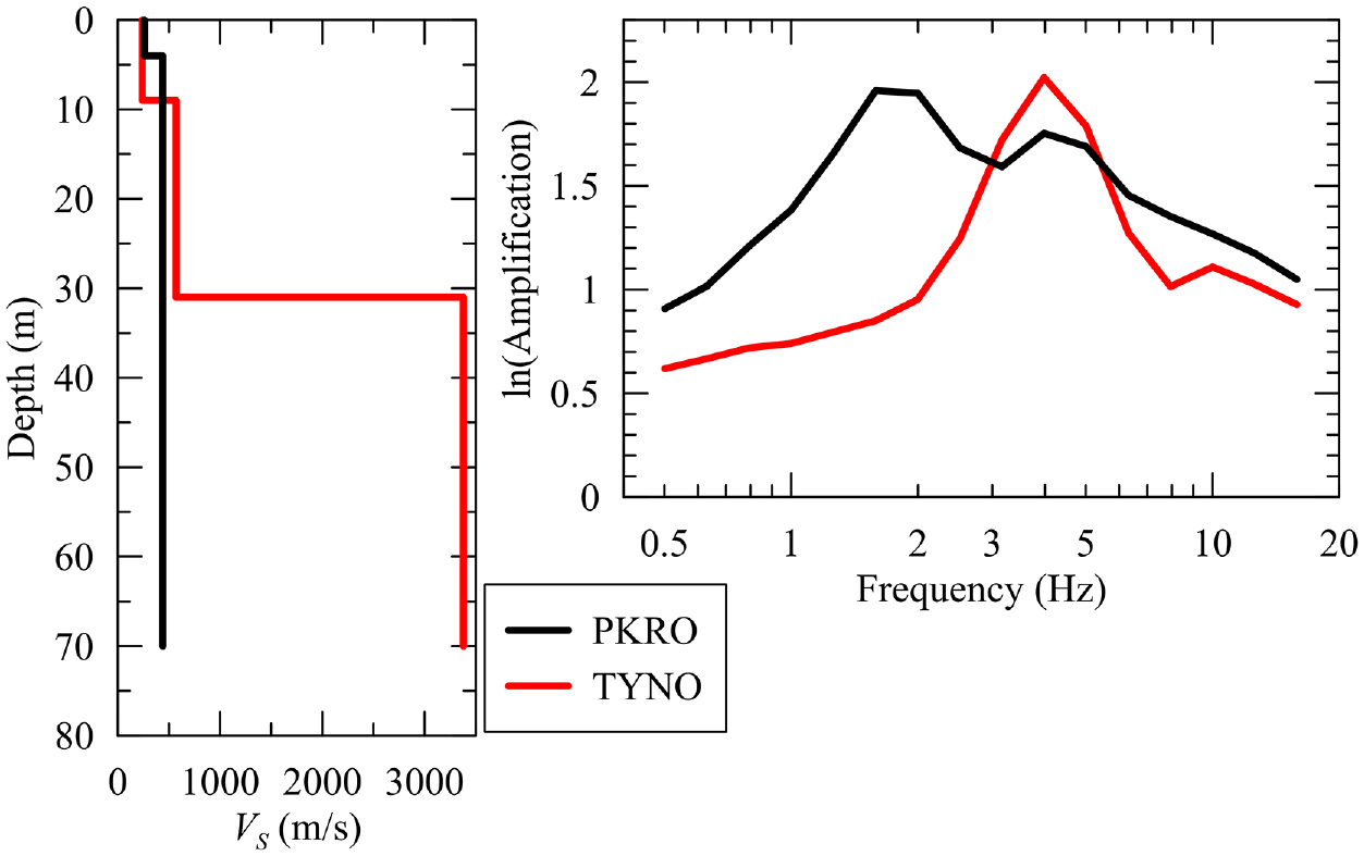
(a) V_S profiles of two sites (TYNO and PKRO) from Beresnev and Atkinson (1997), and (b) natural logarithm of site amplification from mixed-effect regression of residuals of observed ground motion relative to GMM with respect to hard-rock reference condition from Hassani and Atkinson (2016).

Work conducted since the end of the NGA-East project (∼2020) by investigators independent of NGA-East has examined the effects of sediment depth (i.e. from ground surface to V_S horizon of ∼3000–3500 m/s) on site response in the Atlantic coastal plain (CP) and Gulf Coast using newly available maps from Boyd et al. (2022). Those maps demonstrate that sediment depths across the Atlantic and Gulf CP can exceed 10,000 m, which exceeds the maximum depth (1000 m) of randomized V_S profiles in this study as discussed in the next section. These studies employed a reference site approach using earthquake and microseism data, and the results suggest strong effects of sediment depth on low-frequency components of ground motion (Chapman and Guo, 2021; Pratt and Schleicher, 2021). These models are conditioned on depth alone as defined from the Boyd et al. (2022) maps (i.e. V_S30 and T_nat are not used in tandem).

The simulation work by the GWG, which is denoted subsequently as the prior study, consisted of a parametric study of more than 1.7 million linear (L), equivalent-linear (EL), and NL site response analyses (SRA) to represent the variability and uncertainty in site stratigraphy, material properties, and ground motions at CENA sites. The simulations were used to produce several response spectrum (RS) and smoothed Fourier amplitude spectrum (FAS) site amplification functions derived using conventional NL regression methods (Harmon et al., 2019b). Since that work was completed, some limitations have been identified and are addressed here:

• 1. The diversity of CENA site conditions was not fully represented:

•   a. Gradient profiles, which are defined as those that lack a sharp impedance between the reference rock conditions and the overlying material, are known to exist in CENA (Stewart et al., 2020), particularly south of the southern limit of Wisconsin glaciation (Reed and Bush 2005), and were not represented in the generic site profiles.

•   b. Gaps in the distribution of V_S30 and T_nat (site natural period) within the site database (Figure 2(b)) were observed.

• 2. A model for the standard deviation associated with the median model was not developed.

Figure 2.

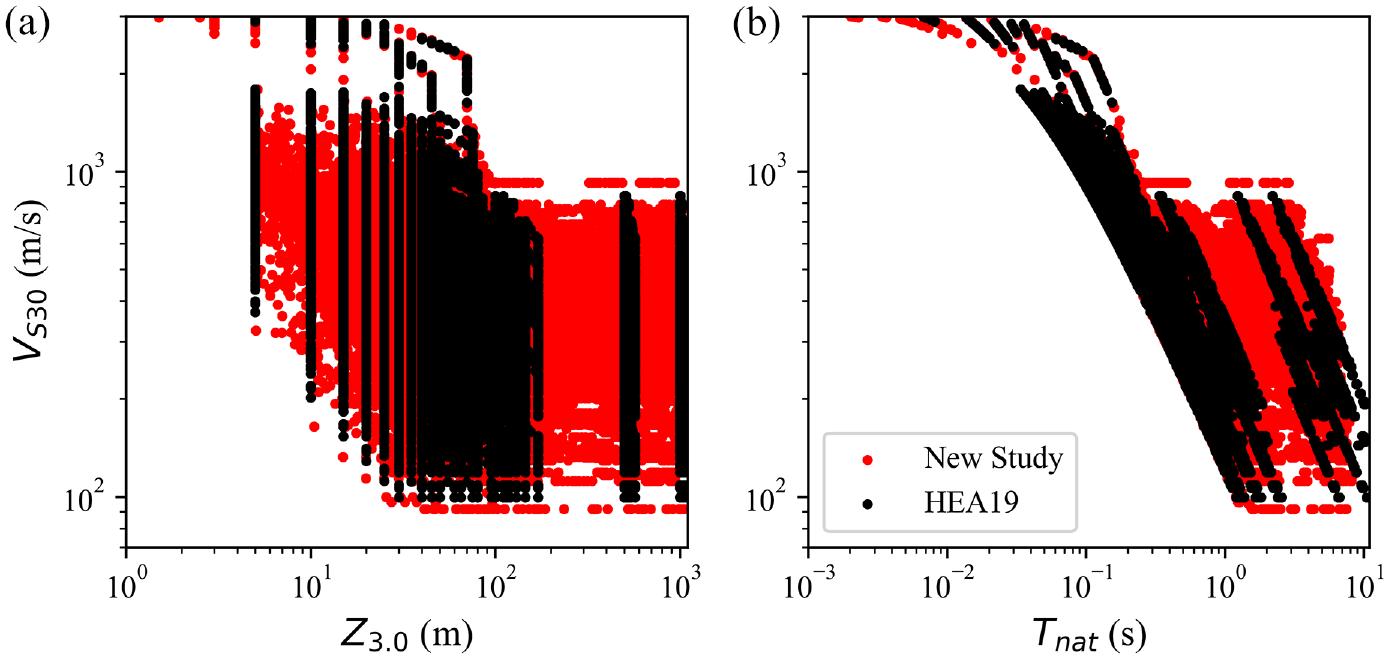
Comparison of site profile databases from Harmon et al. (2019a) and New Study as functions of (a) V_S30 (m/s) and Z_3.0 (m), and (b) V_S30 (m/s) and T_nat (s).

These limitations motivated a second parametric study with additional V_S profiles and updated parameter selection protocols to more accurately represent CENA site conditions and variability from the median predictions. Using these updated simulation results, a new suite of RS and FAS site amplification models is developed to provide functions (this article) and deep learning-based (artificial neural network (ANN)) site amplification models (upcoming article). The models are derived using (1) both V_S30 and T_nat, and (2) only T_nat. Standard deviation relationships that represent the aleatory variability associated with the median model are proposed.

All the models proposed in this article estimate site amplification relative to a V_S = 3000 m/s reference condition. For practical application, amplification factors that convert ground motions applicable to the V_S = 3000 m/s reference condition to ground motions applicable to the softer reference condition of V_S30 = 760 m/s (referred to as F₇₆₀) for both impedance and gradient conditions (Stewart et al., 2020) are suggested.

Site amplification simulation study design

Limitations of prior simulation-based study

The GWG or prior simulation-based study (Harmon et al., 2019a,b; denoted as HEA19) has the following limitations pertaining to the parametric study design:

1. Discrete soil depth (Z_Soil) values were used, which introduce gaps in the parameter space that affect the distributions of profiles when plotted in V_S30-T_nat or V_S30-Z_3.0 (depth to V_S = 3000 m/s) domains. Z_Soil is defined as depth to weathered rock or reference rock.

2. Randomized V_S profiles were derived using the Monte Carlo sampling (MCS) technique (Toro, 1995). This provides no constraint on the tails of the normally distributed random variable, which can cause unreasonably soft or stiff profiles to be generated. Moreover, if a limited number of realizations (e.g. less than 30) are used, the logarithmic mean of the randomized profiles might diverge from the representative seed V_S profile.

3. The procedure used to generate V_S profiles for simulations did not allow for velocity V_S reversals (i.e. a V_S decrease in an underlying layer), which can occur in real sites.

4. All of the seed profiles (i.e. prior to randomization) are underlain by either weathered rock or a hard-rock horizon (V_S = 3000 m/s), leading to significant impedance contrasts in all profiles. However, profiles with a more gradual increase in V_S with depth can occur, particularly below the southern limit of Wisconsin glaciation (e.g. Darragh et al., 2015; Frankel et al., 1996). Such profiles were referred to as gradient V_S profiles in the development of F₇₆₀ models (Stewart et al., 2020).

5. The procedures used to generate V_S profiles through weathered rock zones (WRZs) are unable to capture some sites with high V_S gradients and low WRZ thickness (Hashash et al., 2014).

6. In the development of soil NL properties, shear strength was considered as a limiting shear stress at large shear strains (∼10%). The strength values that were used include cohesion intercepts that are related to V_S. These strengths have been found to be unreasonably high for soil layers at shallow depths.

Needs have also been identified in the formulation of the site amplification functions, including:

1. Amplification functions derived for some profiles have multiple peaks that result from multiple impedance contrasts within the profile. The prior V_S30 and T_nat-based amplification functions are not able to capture these features.

2. The primary conditioning variable in the formulation of the amplification models was V_S30, with other effects (site natural period, depth) modifying the V_S30-conditioned amplification. Because some researchers have advocated for T_nat as the primary site parameter (Hashash et al., 2020a; Hassani and Atkinson, 2016), the model has been formulated with this feature.

3. The HEA19 FAS amplification model required V_S30 and Z_Soil, but due to the lack of Z_Soil parameter for most CENA sites (Bayless, 2019, personal communication), it cannot be used in many practical applications. Hence, FAS models conditioned only on primary site parameters (V_S30 or T_nat) are needed.

4. Standard deviation models are needed for probabilistic applications.

This study updates certain elements of the HEA19 parametric study and functional form to overcome the identified limitations and needs.

New parametric study plan

We adopt the parametric study design of Harmon et al. (2019a), but with significant updates as summarized in Figure 3. The study has two main branches in which the surficial materials are soil or rock (illustrated in the lower and upper parts of Figure 3, respectively). In the soil branch, the generic site profiles consist of three V_S segments: (1) soil, (2) WRZs representative of the transition from soil to bedrock, and (3) a hard-rock reference condition of V_S = 3000 m/s (Hashash et al., 2014). These profiles are developed through V_S randomization using 10 geology-based representative seed V_S profiles, which were originally created in the work by Harmon et al. (2019a). More than 800 V_S profiles from 60 different references (i.e. the literature (Ahdi et al., 2018; Kottke et al., 2023) and open geotechnical reports (Figure A.1) as summarized in Table B1 of Harmon et al. (2019a)) were compiled to develop these profiles. Then, gathered data were classified using the geologic classes proposed in the work by Kottke et al. (2012), and the ultimate seed V_S profiles were produced as detailed in Appendix A.2.1. To assign NL properties to soil layers, the following parameters were considered: (1) index and stress history soil properties (unit weight γ, over-consolidation ratio, soil friction angle ϕ, and plasticity index (PI)); (2) shear modulus G reduction and damping D (MRD) curves, which are conditioned on stresses in combination with properties from (1); (3) soil shear strength, which is used to constrain the large-strain MRD components; and (4) small-strain damping (D_min) values. As a result, the sites in the parametric study, which includes 147,420 unique site profiles, can be described as follows:

• 1 Representative seed V_S profiles, 13 of which are for soil (Figure A.4) and have assigned geology-dependent soil properties (Figure 3) and 3 of which are for WRZ (Figure A.6). These profiles are used as input for V_S statistical randomization (Toro, 1995).

• 2 Thirty random statistical realizations of the V_S profile for each representative seed V_S profile (from Figures A.8 to A.20).

• 3 Three random statistical realizations of modulus reduction (G/G_max) and damping curves (MRD) by Darendeli (2001) for mean, systematically high (+ε), and systemically low (−ε) curves. The MRD randomization is assumed to be independent of the V_S randomization. Shear strength is not randomized.

• 4 Eighteen uniformly distributed bins of soil depth from the ground surface (from 5.0 to 1000 m), Z_Soil, which establish the depth limit of the generic site profiles.

• 5 Seven models to represent the WRZ horizon and corresponding material properties.

Figure 3.

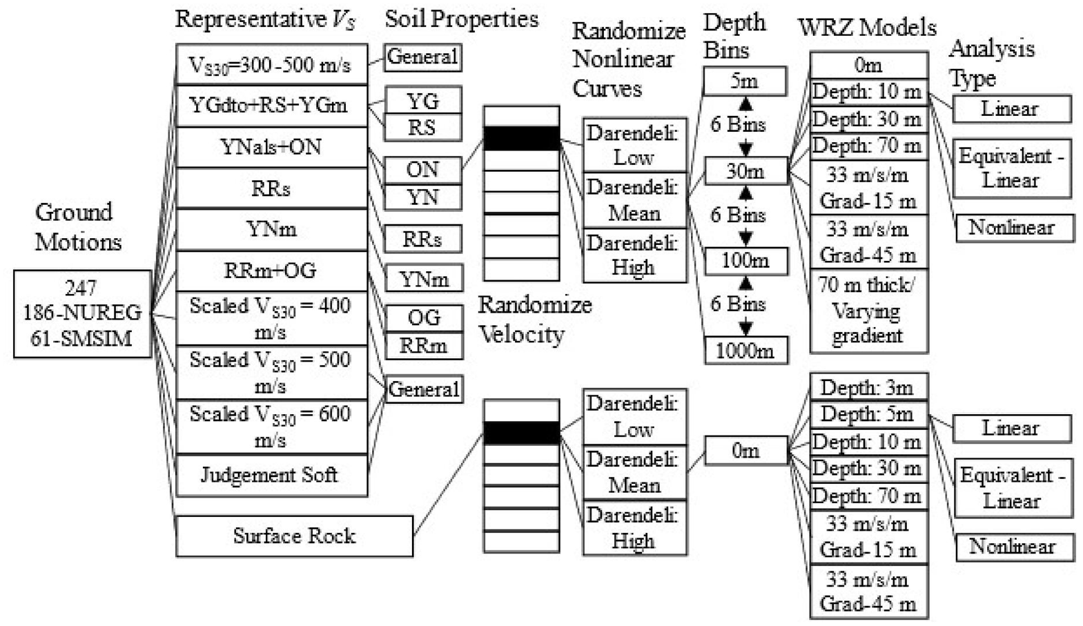
Parametric study tree. Weathered rock zone represents the depth to weathered rock, and the acronyms and abbreviations are presented in Table A.2 of Appendix A.

For near-surface rock conditions (lower branch in Figure 3), the depth to weathered rock, WRZ, is placed at the surface underlain by reference rock. In this branch, 630 unique site profiles are generated, with 3 seed WRZ V_S profiles, 30 V_S profile realizations, and 7 WRZ models. The elements of this branch are similar to those of the upper branch except the truncation of profiles at the uniformly distributed depth bins. All simulations are performed using DEEPSOIL V7.0 (Hashash et al., 2020) in the DesignSafe (Rathje et al., 2017) environment as detailed in Appendix A.4.

In total, the parametric analyses consist of 1,218,945 NL, EL, and linear 1D SRA (for a total of 3,656,835) conducted using 148,050 unique generic site profiles and 247 motions (Appendix A.1) randomly assigned to the site profiles.

Improvements relative to prior parametric study plan

The parametric study described in the previous subsection improves upon that used previously (HEA19) in the following aspects:

1. Uniformly distributed Z_Soil bins are adopted over the depth range of 5–1000 m, resulting in significantly more parameter combinations in V_S30-Z_3.0 space (Figure 2(a)) and V_S30-T_nat space (Figure 2(b)).

2. Latin hypercube sampling (Figure A.7) is introduced into the work by Toro (1995) statistical randomization technique in lieu of MCS to produce randomized V_S profiles whose log-mean is almost equal to or close to the seed V_S profile (Figure 4(b)).

3. V_S reversals (Figure 4(b)) are permitted through an interlayer correlation coefficient (ρ) value of 0.8, which is calculated from collected V_S profiles as given in the work by Ilhan (2020) and is compatible with the value used in the work by Pehlivan et al. (2015).

4. A V_S gradient model, which gradually increases from the bottom of the soil horizon to the top of bedrock and is included in WRZ column of Figure 3, is added to represent gradient V_S profiles. An example of such V_S profile appended to a 55 m deep soil profile is shown in Figure 5, with the other WRZ models used in this study. The linear site response simulations conducted using these profiles are utilized to provide a new set of 760–3000 reference adjustment factors (F₇₆₀).

5. Two new WRZ models (red symbols in Figure A.5) with depths of 3 and 5 m for the near-surface rock branch are added to represent WRZ over bedrock conditions (Figure A.6).

6. A soil strength-V_S relationship from Agaiby and Mayne (2015) is used to more reasonably capture strength profiles at shallow depth (further information in Appendix A.3).

Figure 4.

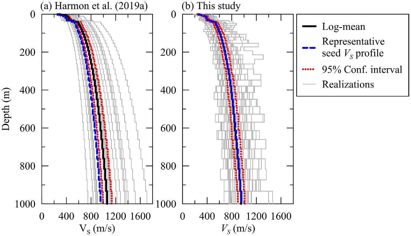
V_S realization of RR representative seed V_S profile with logarithmic mean, 95% confidence interval of the logarithmic mean of V_S realizations, and the representative seed V_S profiles with respect to depth of 1000 m from (a) Harmon et al. (2019a) and (b) New Study. RR: Residual material from metamorphic and igneous rock.

Figure 5.

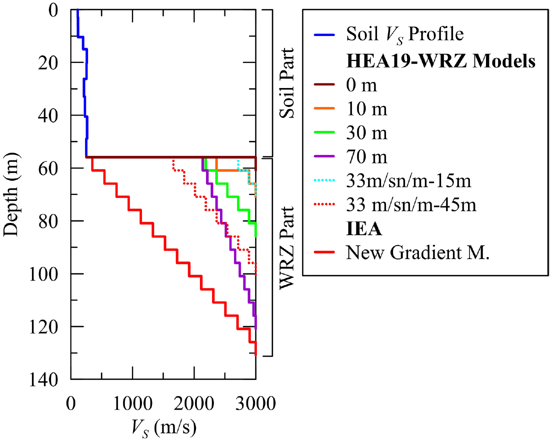
New weathered rock zone model given under IEA title along with models proposed in the work by Harmon et al. (2019a) and Darragh et al. (2015), denoted as HEA19 and DEA15, respectively.

Improvements relative to prior amplification functions

The HEA19 site amplification models are summarized in Table 1. This article updates the HEA19 functions as follows:

1. After observing the constant linear amplification at low-to-mid V_S30 sites for short periods (Figure 6), the functional form of the V_S30-based model (i.e. L1 model) was revised to predict a flat region (L1 in Figure 7(a)). This change was made because the linear RS amplification is approximately flat for ∼120 m/s ≤ V_S30 ≤ 500 m/s.

2. The functional form for the first mode of amplification near the natural period (T_nat) and higher modes now includes a combination of the Ricker wavelet and Gaussian functions, with the latter added to represent second-mode peaks.

3. A new model was developed in which the primary conditioning variable was T_nat for RS and f_nat for FAS. This first-mode period/frequency can be evaluated from a V_S profile or from horizontal-to-vertical spectral ratio (HVSR) data.

4. Tabular values of FAS amplification are replaced with regression equations having the same form as those for RS amplification.

5. Standard deviation (σ) relationships that describe the dispersion of simulation results relative to the median models are developed. The σ model in the work by Hashash et al. (2020a), HEA20, is revised to better represent the dispersion of residuals for NL amplification model.

Table 1

The functional forms of linear RS amplification models in the work by Harmon et al., (2019a)

	Model terms	Functional form
L1 (HEA19)	f(VS30)L1(HEA19)	$\{\begin{array}{c}{V}_c<V_{S30}\hfill \\ V_L<V_{S30}<V_{S30}\hfill \\ V_{S30}<V_L\hfill \end{array}\begin{array}{c}0\hfill \\ \multicolumn{1}{c}{c_1\ln (V_{S30}/V_c)}\\ \multicolumn{1}{c}{c_1\ln (V_{S30}/V_c)+c_2\ln (V_{S30}/V_L)+c_{2}l{n}^2(V_{S30}/V_L)}\end{array}$
L5 (HEA19)	f(VS30)L1(HEA19)+f(Tnat)L1(HEA19)	$f(T_{\mathrm{nat}}{)}_{L1(\mathrm{HEA}19)}=\{\begin{array}{c}{T}_{\mathrm{OSC}}<0.01s\hfill \\ \multicolumn{1}{c}{T_{\mathrm{OSC}}\ge 0.01s}\end{array}\begin{array}{c}{c}_6{T}_{\mathrm{nat}}\hfill \\ \multicolumn{1}{c}{c_5{R}^{*}+c_6{T}_{\mathrm{nat}}}\end{array}$
N2 (HEA19)	f(NL)	Identical to the Equation 11

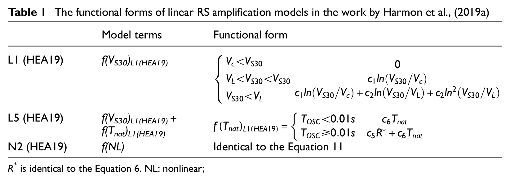
R ^* is identical to the Equation 6. NL: nonlinear;

Figure 6.

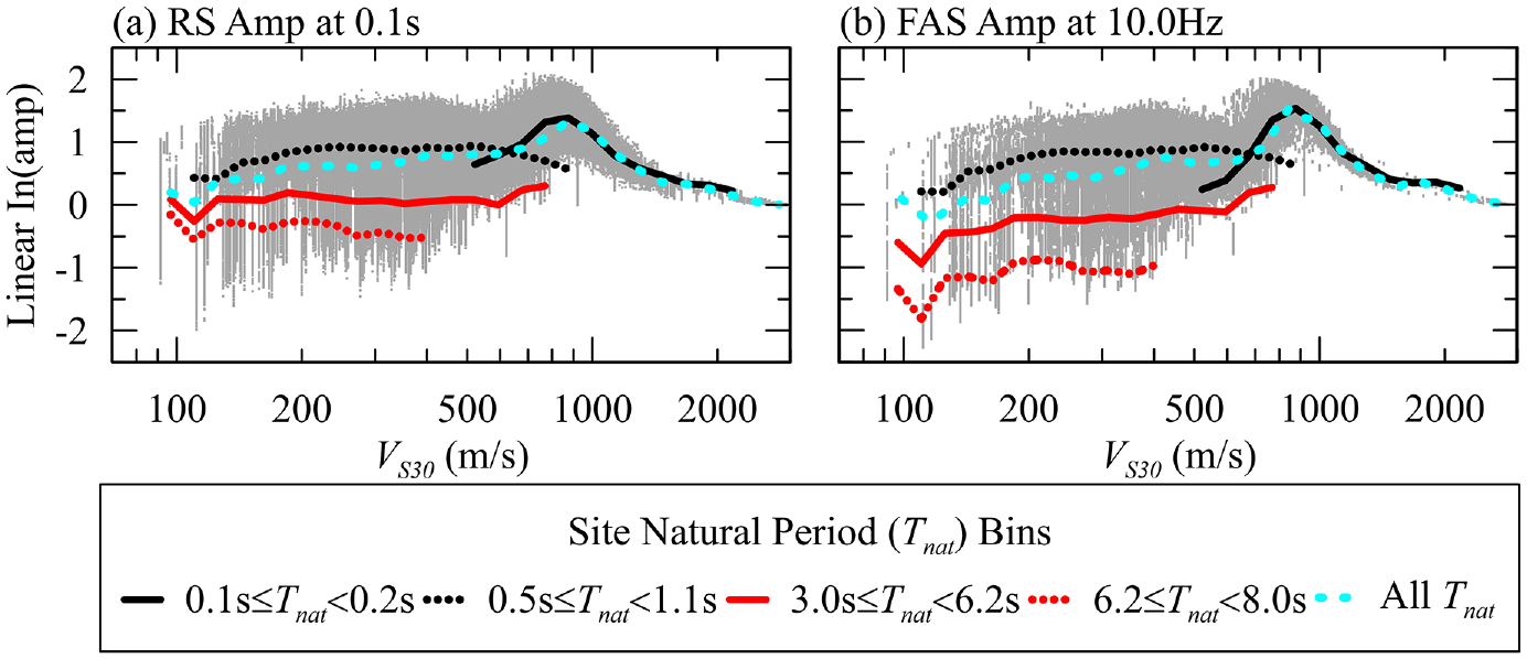
(a) Linear RS ln(amplification) together with the binned mean of linear RS ln(amplification) as function of V_S30 and T_nat for T_OSC of 0.1 s, and (b) linear FAS ln(amplification) along with the binned mean of linear FAS ln(amplification) for V_S30 and F_nat for f of 10.0 Hz. The F_nat bins are the reciprocal of T_nat bins. RS: response spectrum; FAS: Fourier amplitude spectrum.

Figure 7.

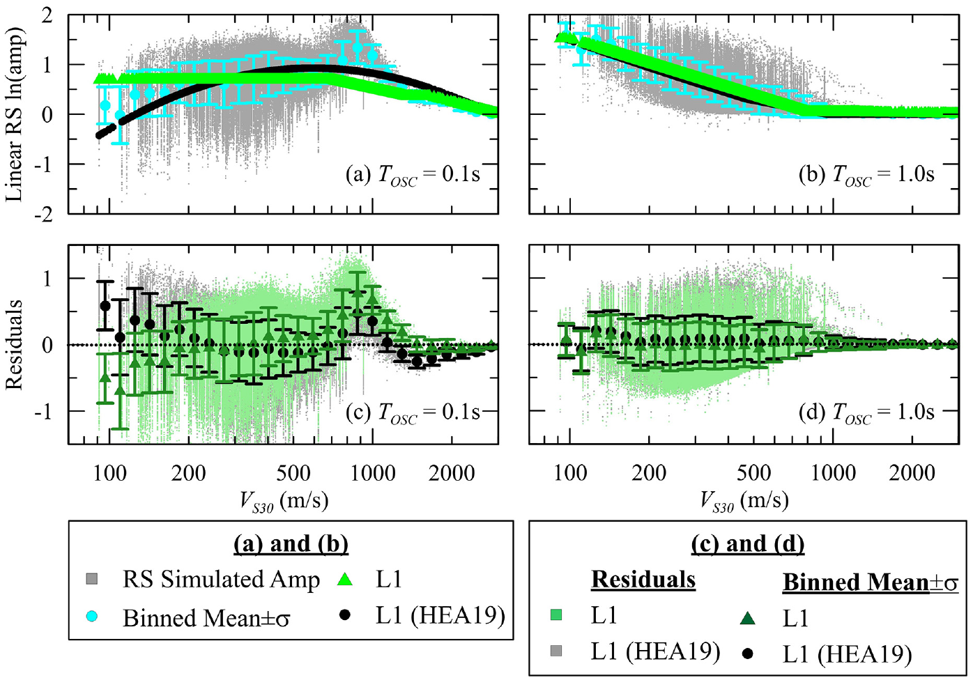
Comparison of estimations from L1 and L1 (HEA19) model calculated using Harmon et al. (2019b) coefficients along with linear response spectrum ln(amplification) and its binned mean ± 1σ for (a) 0.1 s and (b) 1.0 s. The residuals of L1 and L1 (HEA19) models are given for (c) 0.1 s and (d) 1.0 s.

Details of these changes are presented in the following subsections.

RS amplification

The amplification is formulated in natural log units as the sum of linear (F_lin) and NL (F_nl) components (Seyhan and Stewart, 2014):

$$F_S=F_{\mathrm{lin}}+F_{\mathrm{nl}}$$

(1)

The linear component has two model terms, the second of which is optional,

$$F_{\mathrm{lin}}=f(V_{S30})+f(T_{\mathrm{nat}}{)}_{L5}$$

(2)

An alternative form of the linear component is conditioned only on T_nat (similar to Hassani and Atkinson, 2016),

$$F_{\mathrm{lin}}=f(T_{\mathrm{nat}}{)}_{L6}$$

(3)

The NL function, $F_{\mathrm{nl}}$ , represents the NL site amplification as a function of soil stiffness and ground motion intensity parameters. Equations for each of the model components, $f(V_{S30})$ , $f(T_{\mathrm{nat}})$ , and $F_{\mathrm{nl}}$ , are provided in the following subsections. The coefficients in those equations are fit using simulation results from the new parametric study. Table 2 summarizes the components of the L, NL, and total amplification functions.

Table 2.

List of all RS and FAS site amplification models

Model terms	Model type	Simultaneous regression	Sequential regression
f(VS30)	Linear	L1	—
f(VS30) + f(Tnat)	Linear	L5	—
f(Tnat)	Linear	L6	—
f(VS30) + f(NL)	Total (SA) and envelope (E)		L1 + N1 a , L1 + N1 a (E)
f(VS30) + f(Tnat)|f(fnat) b  + f(NL)	Total (SA) and envelope (E)	K1 a , K1 a (E)	L5 + N1 a , L5 + N1 a (E)
f(VS30) + f(NL)	Total (PGA) and envelope (E)		L1 + N2, L1 + N2 (E)
f(VS30) + f(Tnat)|f(fnat) b  + f(NL)	Total (PGA) and envelope (E)	K2, K2 (E)	L5 + N2, L5 + N2 (E)

a

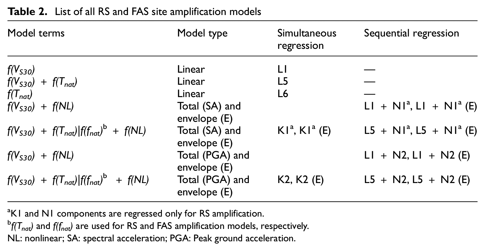
K1 and N1 components are regressed only for RS amplification.

b

f(T_nat) and f(f_nat) are used for RS and FAS amplification models, respectively.

NL: nonlinear; SA: spectral acceleration; PGA: Peak ground acceleration.

V_S30 scaling

V_S30 is commonly used as an independent variable in site amplification functions (e.g. Borcherdt, 1994; Parker et al., 2019). The V_S30-based L1 model (in which V_S30 is the sole site parameter) is given as,

$$f\left(V_{S30}\right)=\{\begin{array}{c}c·\ln (V_1/V_b)V_{S30}\le V_1\hfill \\ c·\ln (V_{S30}/V_b)V_1<V_{S30}\le V_2\hfill \\ c·\ln (V_2/V_b)V_2<V_{S30}\le V_u\hfill \\ c·\ln (V_2/V_b)[1-\ln (V_{S30}/V_u)/\ln (3000/V_u)]V_u<V_{S30}<3000m/s\hfill \end{array}$$

(9)

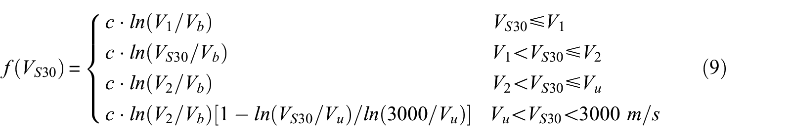
where c is the slope of the model component producing linearly varying ln(amplification) with ln(V_S30) between corner velocities of V₁ and V₂, V_b and V_u are the model coefficients that vary with period. Constant amplification is modeled for V_S30 less than V₁, replacing the decay function (i.e. decreasing amplification as V_S30 decreases) in HEA19, and constant amplification (constrained by simulations) is also modeled at V_S30 greater than V₂. For V_S30 greater than V_u, the amplification decreases linearly to 0.0 between V_u and 3000 m/s. Equation 4 is modified from the F_V term (representing V_S30 scaling) given by Stewart et al. (2020) (denoted as SEA20) but with V_ref (760 m/s) in SEA20 replaced with V_b in Equation 4.

Figure 6(a) shows trends of simulated amplification results for 0.1 s RS as a function of V_S30. The figure shows binned means for all results and for sites with selected values of T_nat; the T_nat results are addressed in the next subsection. The overall results in Figure 6(a) show that the amplification is constant with respect to V_S30 for 150 m/s ≤ V_S30 ≤ 750 m/s as represented by the first term in Equation 4 (this behavior is also observed for bins of T_nat ≤ ∼1.1 s, but not for some higher periods). Notably, this V_S30-independent amplification is not observed in empirical data (Parker et al., 2019). However, the focus of this article is on fitting the simulated data and not on V_S30 models that would be recommended for application. For higher velocities, the overall site amplification reduces linearly with ln(V_S30) and is represented by the second and fourth terms in Equation 4.

Figure 7(a) and (b) compares the L1 estimates from Equation 4 and from the model of HEA19 for T_OSC (oscillator periods) of 0.1 and 1.0 s. Even though these models are similar for T_OSC of 1.0 s (Figure 7(b)), the HEA19 L1 model significantly deviates from the L1 model of this study at T_OSC ≤ 0.1 s due to the decay in ln(amplification) for low V_S30 sites. At T_OSC = 0.1 s, the L1 and L1 (HEA19) models are biased positive and negative, respectively, relative to the simulated amplifications at V_S30 < 200 m/s (Figure 7(c)), and both models are unable to capture the peak amplification around V_S30 = 1000 m/s. The observable bias in L1 estimations is anticipated since it does not include T_nat term in its functional form and is, therefore, unable to capture influences of site resonances, which have the effect of reducing amplification at low V_S30 sites at illustrated in Figure 6(a). This is addressed in subsequent sections by enhancing the model through the use of the T_nat parameter, both in the V_S30-scaling model (as depicted in Figure 6) and by the introduction of peaks in the amplification function (resonance effects). The coefficients of the L1 model are presented in Figure B.1.

T_nat effects

The trend of site amplification with V_S30 is T_nat-dependent, as can be seen in Figure 6(a). In the case of short-period RS, as T_nat increases, the amplification decreases, which is caused by increased material damping from deeper profiles. However, we argue that amplification effects related to T_nat should principally be directed toward the modeling of peaks related to site resonances and with the decay in amplitudes that reflect cumulative damping effects that depend on soil depth. As described in the previous section, the 1D simulations were performed using two types of profiles: (1) impedance and (2) gradient sites. The former is expected to produce a peaked response due to resonance effects caused by the existence of a sharp impedance contrast between the WRZ, or reference rock of V_S = 3000 m/s (Hashash et al., 2014), and the overlying soil material.

Justification for the addition of the G component of the model in Equation 5 is provided by plotting residuals of the V_S30-scaling model (L1) versus $T_{\mathrm{OSC}}/T_{\mathrm{nat}}$ as shown in Figure 8(a). The residuals demonstrate a pattern of behavior in which (1) a first-mode peak occurs at $T_{\mathrm{OSC}}\approx 0.81T_{\mathrm{nat}}$ ; (2) a second-mode peak occurs at $T_{\mathrm{OSC}}\approx 0.31T_{\mathrm{nat}}$ ; (3) amplification decays (shorter periods) for $T_{\mathrm{OSC}}<0.31T_{\mathrm{nat}}$ ; and (4) amplification falls off the peak to a dip and then flattens for $T_{\mathrm{OSC}}>0.81T_{\mathrm{nat}}$ (longer periods). The HEA19 model using only Ricker wavelet to represent the first-mode peak can capture most of this complex behavior, except for the peak at $T_{\mathrm{OSC}}\approx 0.31T_{\mathrm{nat}}$ (Figure 8(b)), and it is for this reason that Equation 5 adds the Gaussian term at $T_{\mathrm{OSC}}\approx 0.31T_{\mathrm{nat}}$ . The improved fit using this term is illustrated in Figure 8(b).

Figure 8.

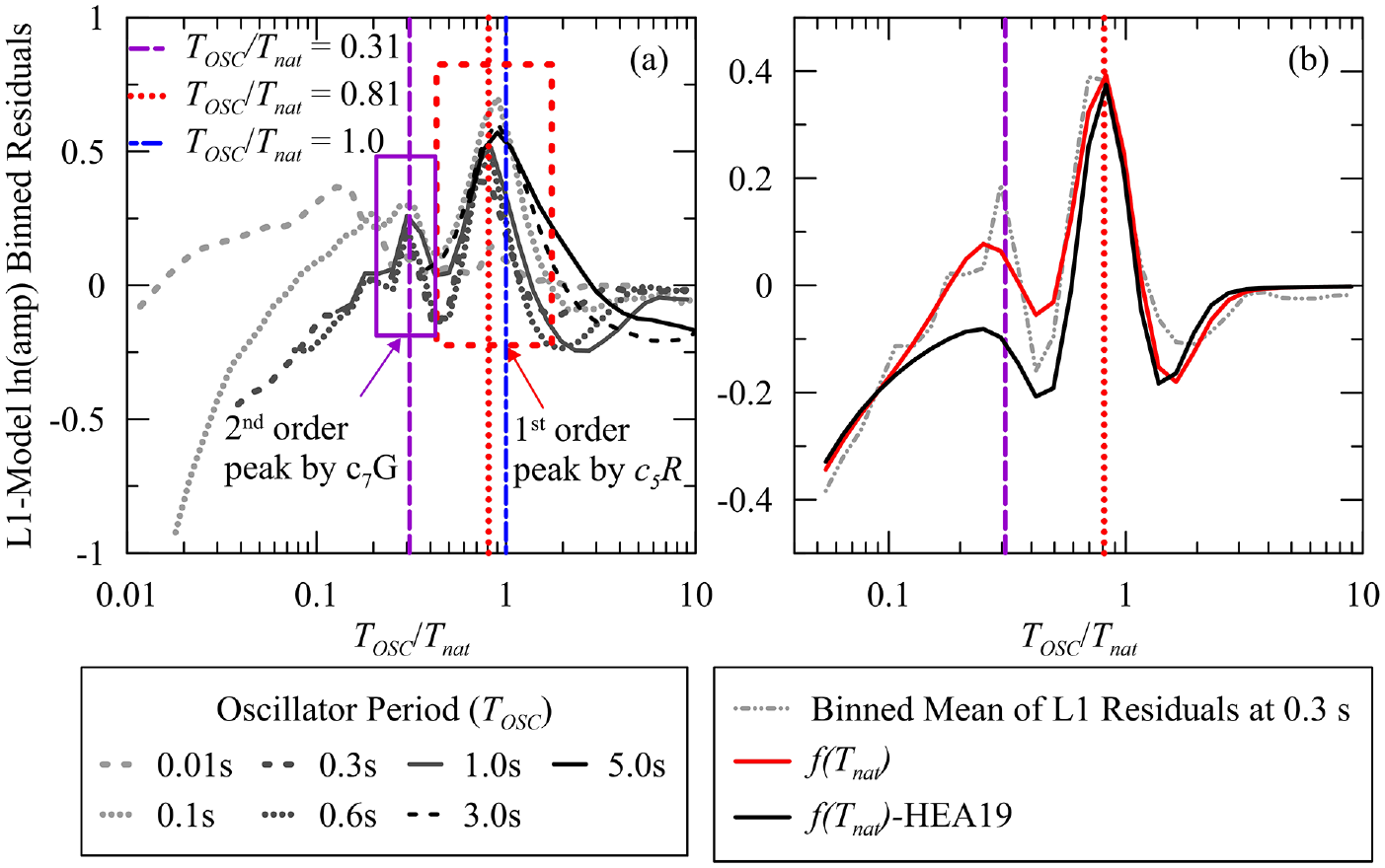
(a) The binned residuals of the L1 response spectrum model computed as the difference between linear ln(amplification) and L1 estimations as a function of T_OSC/T_nat for T_OSC of 0.01, 0.1, 0.3, 0.6, 1.0, 3.0, and 5.0 s, and (b) the residuals of the L1 as a function of T_OSC/T_nat for T_OSC of 0.3 s along with f(T_nat) and f(T_nat)-HEA19 model estimations.

For the modeling of T_nat effects on site amplification, a framework is adopted from HEA19, in which the amplification from a V_S30-only model (Equation 4) is modified using a period-dependent equation. HEA19 used a Ricker wavelet centered near T_nat with ramp functions at shorter and longer periods. That approach is updated here by adding a second-mode peak that is assumed to occur at 0.31T_nat and is described by a Gaussian function. The model is formulated as follows:

$$f(T_{\mathrm{nat}}{)}_{L5}=\{\begin{array}{c}{c}_6{T}_{\mathrm{nat}}\hfill \\ c_{5}R+c_6{T}_{\mathrm{nat}}+c_{7}G\hfill \\ c_{5}R+c_6{T}_{\mathrm{nat}}\hfill \end{array}\begin{array}{c}{T}_{\mathrm{OSC}}<0.01s\hfill \\ 0.01s\le T_{\mathrm{OSC}}\le 3.0s\hfill \\ T_{\mathrm{OSC}}>3.0s\hfill \end{array}$$

(5)

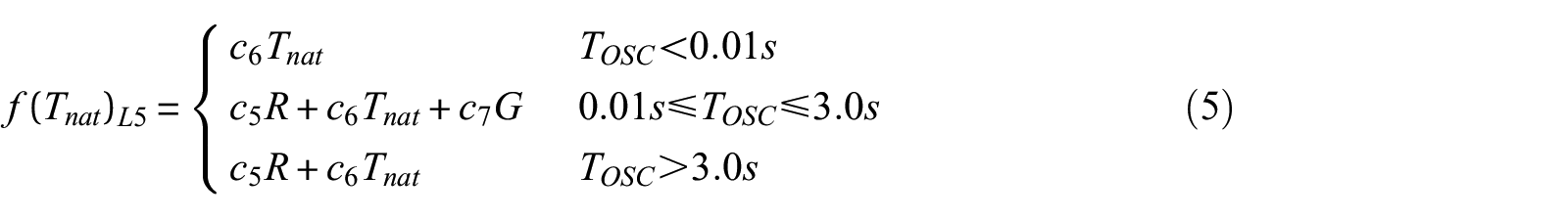
where c₅, c₆, and c₇ are period-dependent coefficients, and R is the Ricker wavelet term to capture the first-mode peak amplification at T_OSC/T_nat≈ 0.81 together with two troughs next to it:

$$R=\frac{2}{\sqrt{3{\alpha }_1}{\pi }^{0.25}}·(1-\frac{{\beta }_1^2}{{\alpha }_1^2})·\exp (-\frac{{\beta }_1^2}{2{\alpha }_1^2})$$

(6)

and the second-mode peak is captured by Gaussian term denoted as G:

$$G=\frac{1}{{\alpha }_2\sqrt{2\pi }}·\exp [-\frac{1}{2}·{\left(\frac{{\beta }_2}{{\alpha }_2}\right)}^2]$$

(7)

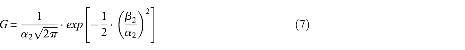
where α₁ and α₂ are period-dependent regression coefficients, and β₁ and β₂ are given as:

$${\beta }_1=\ln \left(\frac{T_{\mathrm{OSC}}}{T_{\mathrm{nat}}}\right)-\ln (0.81),{\beta }_2=\ln \left(\frac{T_{\mathrm{OSC}}}{T_{\mathrm{nat}}}\right)-\ln (0.31)$$

(8)

The G component is only applied for T_OSC < 3.0 s since the second mode of peak amplification seems to disappear for T_OSC > 3.0 s (Figure 8(a)).

Figure 9(a)–(d) compares computed amplifications for the L5 model in this study and HEA19 and the residuals of L5 models, respectively, for T_OSC of 0.1 and 1.0 s. The linear amplification data are plotted as dispersed points in log(V_S30) space since each randomized profile terminates at different depths beyond 30.0 m (Figure 3), resulting in profiles with the same V_S30 but different T_nat values, and thus different amplifications. As expected, this condition is observed in L5 estimations. The only appreciable differences between the two generations of L5 models are for 100 m/s ≤ V_S30 ≤ 200 m/s; the updated model provides residuals closer to zero. The amplification behavior in this V_S30 region is strongly influenced by profile damping, which is captured much better when T_nat is included as an independent variable. For V_S30 > 200 m/s, simulation results and model fits are similar. The coefficients for f(V_S30) and f(T_nat)_L5 are illustrated in Figures B.1 and B.2, respectively.

Figure 9.

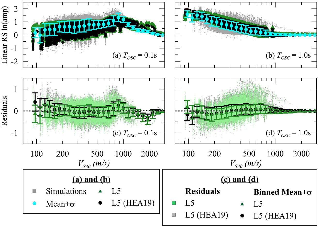
Comparison of estimations from L5 and L5 (HEA19) model calculated using Harmon et al. (2019b) coefficients (HEA19) along with linear response spectrum ln(amplification) and means of ln(amplification) ± 1σ for (a) 0.1 s and (c) 1.0 s. The models’ residuals with their means ± 1σ are given for (c) 0.1 s and (d) 1.0 s.

Model with T_nat as primary independent variable

As noted previously, an alternative to the L5 model (Equations 4 and 5) in which T_nat is used as the only independent variable (Equation 3) is provided. Denoted as L6, the form of the model was selected based on inspections of amplification plots (relative to reference rock) as shown in Figure 10(b), in which the mean of amplification for soil over bedrock sites and WRZ over bedrock site is plotted with respect to log(T_OSC/T_nat). Two principle trends are observed:

1. Soil sites: These sites characteristically have a region with a series of peaks and troughs associated with T_OSC ∼ T_nat and T_OSC < T_nat (i.e. first and higher modes of the site) along with an amplification decay region at short periods (T_OSC << T_nat) due to soil-damping effects. These trends are similar to those observed in the mean of L1 model residuals (Figure 10(a)).

2. WRZ sites: Amplification decreases with increasing log(T_OSC/T_nat), which is distinct behavior relative to that at soil sites.

Figure 10.

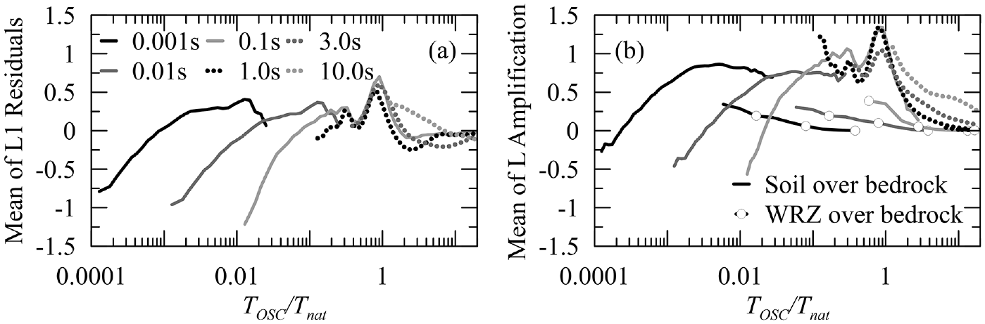
Comparison of (a) L1 model residuals for all sites and (b) binned mean of linear amplification at soil and weathered rock zone sites in T_OSC/T_nat space for T_OSC of 0.001, 0.01, 0.1, 1.0, 3.0, and 10.0 s.

Given the different trends, separate relationships for amplification of soil and WRZ sites were developed. The soil model, denoted f(T_nat)_{L6, Soil}, is formulated as:

$$f{(T_{nat})}_{L6,Soil}=\{\begin{array}{cc}{T}_{OSC}<0.01s& c_{6,1}{T}_{nat}^2+c_{6,2}{T}_{nat}+c_{6,3}\\ 0.01s\le T_{OSC}\le 3.0s& c_{5}R+c_{6,1}{T}_{nat}^2+c_{6,2}{T}_{nat}+c_{6,3}+c_{7}G\\ T_{OSC}>3.0s& c_{5}R+c_{6,1}{T}_{nat}^2+c_{6,2}{T}_{nat}+c_{6,3}\end{array}$$

(9)

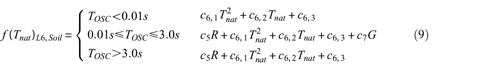
This model is an updated version of f(T_nat)_L5 using a second-order polynomial (i.e. the component with c_6,i coefficients) to better capture the decay in amplification due to soil-damping effects and the shape of amplification at very short periods (e.g. for T_OSC of 0.001 s in Figure 10(b)). The resulting fit to the amplification data and the model’s residuals are shown in Figure 11(a)–(d), respectively, and these plots show an excellent fit to the data.

Figure 11.

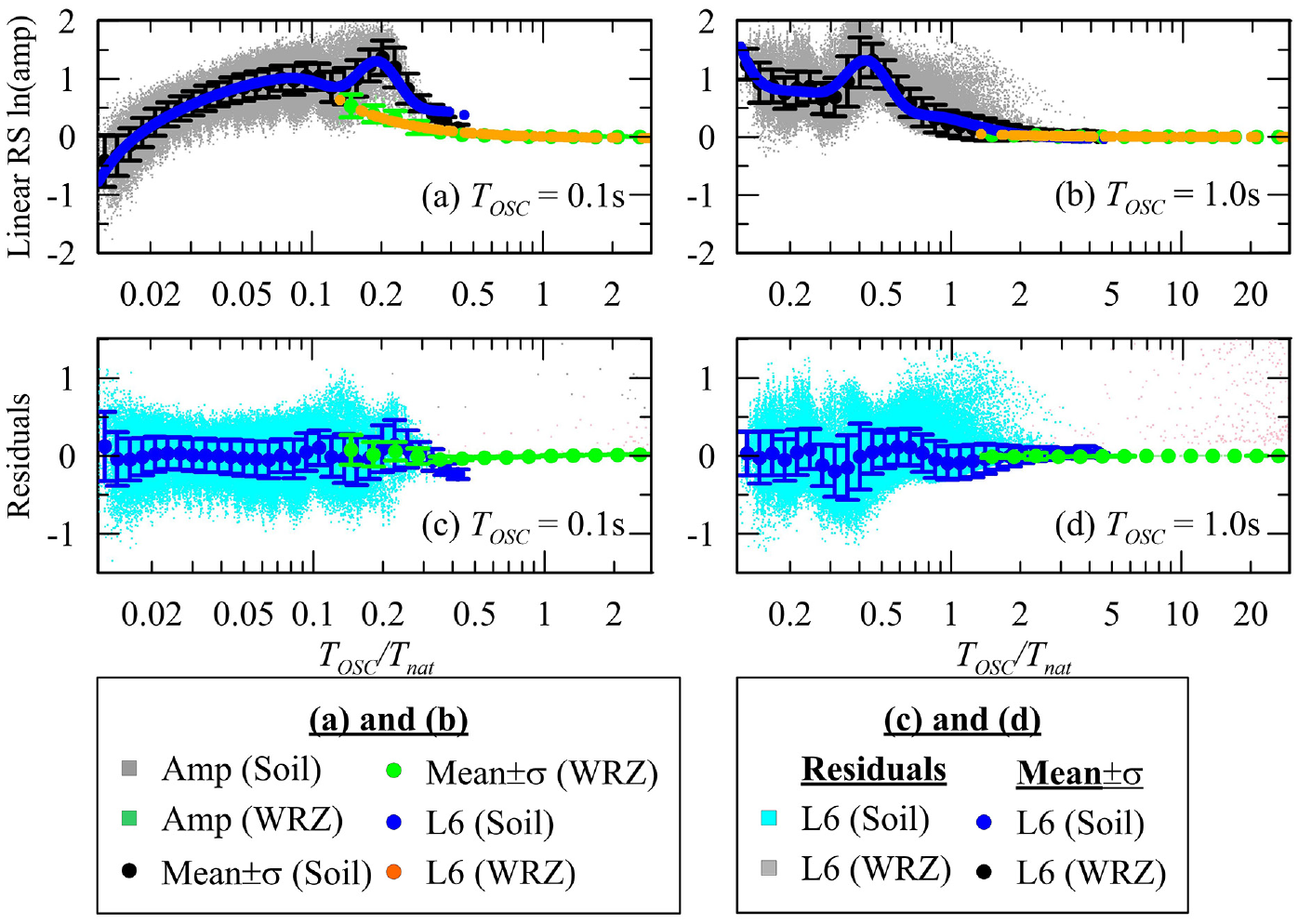
L6 model (both for soil weathered rock zone site amp) and linear response spectrum ln(amplification) along with its binned mean ± 1σ in evenly distributed log(T_OSC/T_nat) space for T_OSC of (a) 0.1 s and (b) 0.1 s. The residuals are given for T_OSC of (c) 0.1 s and (d) 1.0 s.

For WRZ sites, the amplification function is given as,

$$f(T_{\mathrm{nat}}{)}_{L6,\mathrm{WRZ}}=t_5·T_{\mathrm{nat}}+t_6$$

(10)

where t₅ and t₆ are period-dependent coefficients. Figure 11 also illustrates this model and its residuals, which are shown to be very close to zero. The coefficients of L6 models are plotted in Figures B.3 and B.4. The WRZ model (Equation 10) should be used for profiles that lie within the V_S30 and T_nat parametric ranges of WRZ profiles in this study, which are V_S30 > 1000 m/s and T_nat < 0.1 s (Figure 2). Otherwise, the soil model (Equation 9) would apply.

NL and total amplification

HEA19 accounts for NL amplification (F_nl) using the difference between NL and L SRA and omits the EL analyses due to its tendency to overdamp high-frequency components (especially for frequencies (f) > 2.0 Hz; Kim et al., 2016). However, NL analyses produce lower spectral ratios (ratio of spectral acceleration (SA_r) at ground surface to that of input motion) than those from EL because of phase incoherence introduced by NL for f > 25.0 Hz (Rathje and Kottke, 2011). Thus, the envelope of NL and EL SRA is adopted such that the maximum of the surface response is taken across all T_OSC to avoid reductions in NL amplification at large frequencies. This indicates that two different sets of amplification results can be considered, as follows:

1. NL amplification: (a) The difference between NL and L SRA, and (b) the difference between the envelope of NL and EL simulations, which is denoted as envelope, and L SRA

2. Total amplification: (a) NL and (b) enveloped results

$F_{\mathrm{nl}}$ is formulated identically to HEA19b,

$$F_{nl}=\{\begin{array}{cc}{f}_{2}ln\left(\frac{I_r+f_3}{f_3}\right)& V_{S30}<V_c\\ 0& V_{S30}\ge V\end{array}$$

(11)

where I_r represents the outcropping rock motions (V_S = 3000 m/s) in one of two possible forms—SA_r for a given T_OSC or PGA at rock (PGA_r) (these models are denoted as N1 and N2, respectively) and f₂ is a coefficient that associates the degree of nonlinearity with the stiffness of the site and is given as (modified from Chiou and Youngs, 2008),

$$f_2=f_4[\exp \left\{f_5(\min (V_{S30},V_{\mathrm{ref}})-360)\right\}-\exp \left\{f_5(V_{\mathrm{ref}}-360)\right\}]$$

(12)

where f₃ represents the transition ground motion level from linear to NL site amp, and I_r is an intensity measure that represents the strength of the ground motion for reference rock conditions (V_S = 3000 m/s). V_c is the velocity at which no amplification occurs relative to V_S = 3000 m/s and comes from the L1 model regressions.

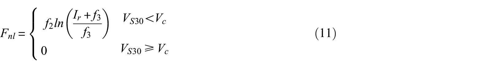
Figure 12(a) and (c) shows the NL-L amplification data as functions of V_S30 and PGA_r and fits from Equations 13 and 14. Some oscillations with respect to PGA_r occur in the data due to different numbers of data points for different PGA_r intervals. The fitted model from this study is compared with that from HEA19b, which generally provides similar results, although more nonlinearity is now predicted for V_S30 (m/s) and PGA_r (g) pairs less than (110, 0.35), (175, 0.45), and (270, 0.6) for 0.1 s. The N2 model is applied to the Envelope-L data set as given in Figure 12(b) and (d), producing larger amplification (less nonlinearity) relative to NL-L analyses. Using N2 coefficients regressed through the Envelope-L data provides future users with the option of working with larger amplification values. The residuals and the coefficients of N2 relationships are presented from Figures B.8 to B.11.

Figure 12.

The estimations from N2 and N2 (HEA19) models for response spectrum NL site ln(amplification) from (a and c) the difference between NL and L simulations (NL-L analyses) and from (b and d) the difference between the envelope of NL and equivalent-linear (EL) simulations and L analyses (Envelope-L analyses) along with corresponding simulated amplification data (i.e. binned mean of amplification data) as functions of V_S30 and PGA_r for oscillator periods of 0.3 and 1.0 s. NL: nonlinear.

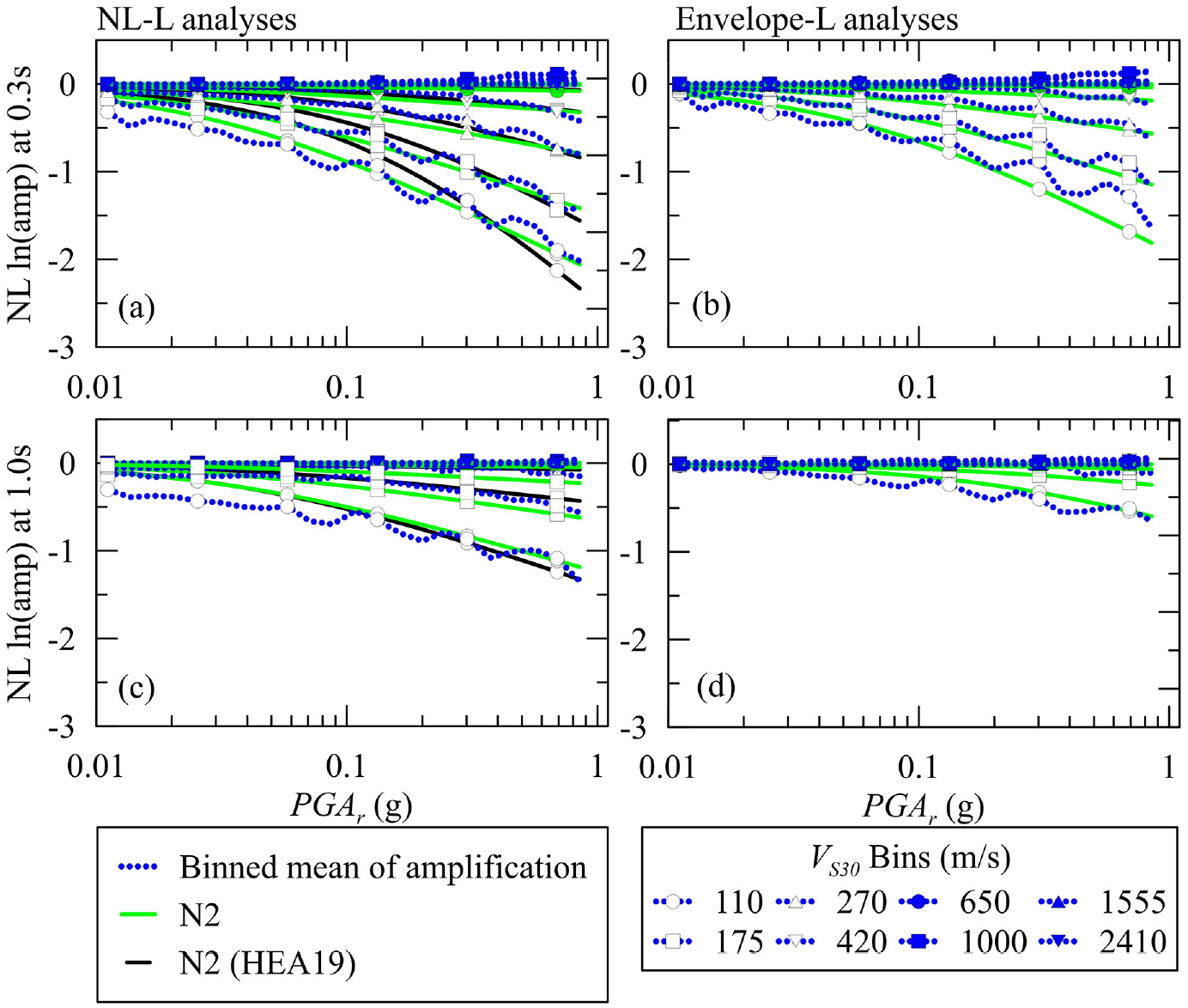
The total amplification estimates from L5 + N2 (this study) and L5 + N2 (HEA19) are assessed in Figure 13 for T_OSC of 0.1 and 1.0 s. The enhancements of L5 + N2 (this study) over L5 + N2 (HEA19) are limited such that the binned mean residuals from the new model are slightly closer to zero at 200 m/s < V_S30 < 400 m/s and 120 m/s < V_S30 < 150 m/s for 0.1 and 1.0 s, respectively. In addition to L5 + N functions, K models defined in Table 2 and the N function using NL-L and Envelope-L amplification are discussed in Appendix B.1.

Figure 13.

Comparison of estimations from L5 + N2 and L5 + N2 (HEA19) computed using Harmon et al. (2019b) coefficients along with total response spectrum ln(amplification) from nonlinear simulations and its binned mean ± 1σ for (a) 0.1 s and (b) 1.0 s. In addition, the models’ residuals are presented for (c) 0.1 s and (d) 1.0 s.

FAS amplification

The natural log of the FAS amplification (E_S) is defined as the sum of modular linear (E_lin) and NL amplification (E_nl) terms in a similar manner to RS amplification,

$$E_S=E_{\mathrm{lin}}+E_{\mathrm{nl}}$$

(13)

The same functional forms are used for FAS amplification components as described previously for RS amplifications, based on the similarity of the data sets (Figure 6 and Figure B.21 for linear and NL, respectively). For the T_nat-effect models, L5 is re-cast using the independent variable of natural frequency ( $F_{\mathrm{nat}}$ ) in lieu of T_nat and frequency in lieu of oscillator period,

$$f(F_{\mathrm{nat}})=\{\begin{array}{c}f\le 0.33\mathrm{Hz}\hfill \\ 0.33\mathrm{Hz}<f<33.0\mathrm{Hz}\hfill \\ f\ge 33.0\mathrm{Hz}\hfill \end{array}\begin{array}{c}{c}_{5}R+c_6/F_{\mathrm{nat}}\hfill \\ c_{5}R+c_6/F_{\mathrm{nat}}+c_{7}G\hfill \\ c_{5}R+c_6/F_{\mathrm{nat}}\hfill \end{array}$$

(14)

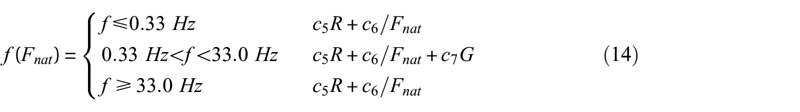
where R and G terms are analogous to the Equations 6 and 7, respectively, and β₁ and β₂ in the R and G terms of Equation 14, respectively, are given as,

$${\beta }_1=\ln \left(\frac{f}{F_{\mathrm{nat}}}\right)-\ln \left(\frac{1.0}{0.81}\right),{\beta }_2=\ln \left(\frac{f}{F_{\mathrm{nat}}}\right)-\ln \left(\frac{1.0}{0.31}\right)$$

(15)

The coefficients of the f(V_S30) part of the L5 model are given in Figure B.25.

Figure 14 compares L5 and tabulated values of HEA19 as functions of V_S30 and Z_Soil for frequencies of 10 and 1.0 Hz. L5 seems to reasonably capture the overall linear FAS amplification, although the residuals of L5 exhibit fluctuations across the V_S30 space indicating the model’s inability to capture the complex trends in the FAS amplifications. We considered adding additional terms to Equation 14 to bring the binned means of residuals closer to zero, but ultimately decided against this to avoid over-complicating the functional form and introducing coefficients that might be poorly constrained. There are two issues related to the use of the HEA19 model: (1) the Z_Soil information might not be available for sites of interest, and (2) the tabulated values of V_S30 and Z_Soil do not seem to cover the data space accurately. Thus, a continuous L5 model conditioned on V_S30 and T_nat is preferred over HEA19. The attributes of the F_nat-only relationship (L6) and NL and total FAS amplification models are discussed in Appendix B.2.

Figure 14.

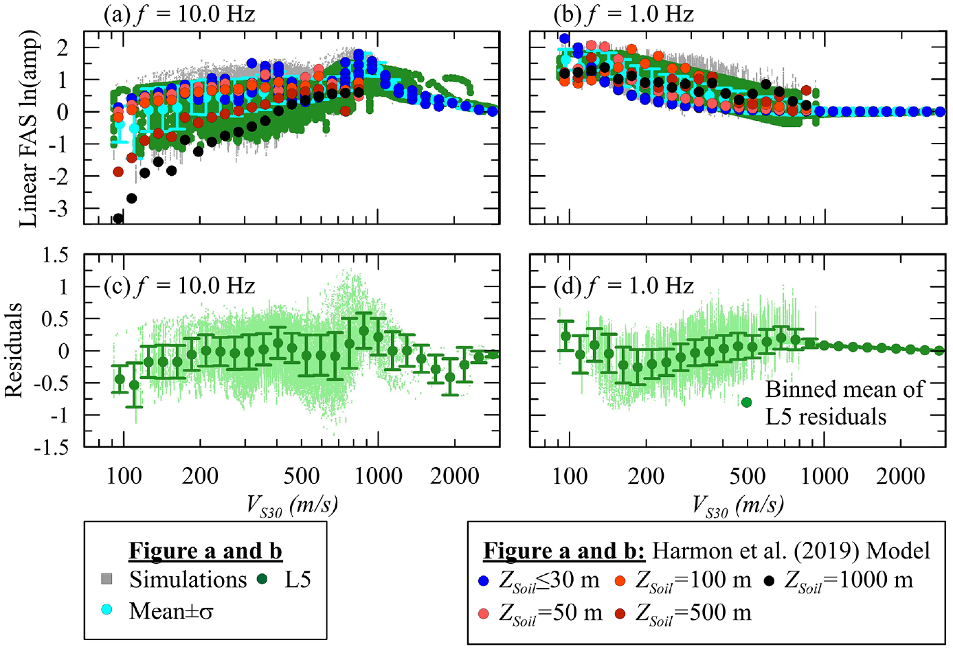
Comparison of estimations from L5 and L5 (HEA19) tabulated values as functions of V_S30 and Z_Soil, and along with linear Fourier amplitude spectrum ln(amplification) and its binned mean ± 1σ for (a) 10.0 Hz and (b) 1.0 Hz. In addition, the models’ residuals are presented for frequency (f) of (c) 10.0 Hz and (d) 1.0 Hz.

Reference site correction factors from 760 to 3000 m/s condition

In the development of ergodic site amplification models for practical application, both empirical and simulation-based results are considered (Stewart et al., 2020). The empirical models are able to predict relative levels of amplification within the range over which the independent variable occurs at ground motion recording sites. The primary independent variable that is considered is V_S30, and its range of observed values in CENA is about 200 to 2000 m/s (Parker et al., 2019). This presents practical difficulties in predicting site response relative to the 3000 m/s reference condition. To overcome this problem, empirical amplification studies have evaluated amplification relative to the NEHRP B-C boundary (760 m/s), which is comfortably within the data range and is sufficiently stiff that complexities associated with NL site response are unlikely to be significant. Within this framework, amplification relative to V_S = 3000 m/s is taken as the log sum of amplification relative to 760 m/s and amplification for sites with V_S30 = 760 m/s relative to the reference condition V_S = 3000 m/s (denoted as F₇₆₀),

$$\ln (\mathrm{amplification}{)}_{3000}=\ln (\mathrm{amplification}{)}_{760}+F_{760}$$

(16)

where ln(amplification)₃₀₀₀ and ln(amplification)₇₆₀ are the natural logarithm of linear RS amplification relative to 3000 and 760 m/s, respectively. To be clear, ln(amplification)₃₀₀₀ has the same physical meaning as $F_S$ in Equation 1.

The NSHM (Petersen et al., 2020) uses models for F₇₆₀ that are derived from a series of simulations using two groups of soil profiles, one with strong impedance contrasts and another with relatively gradual increases of stiffness with depth (Stewart et al., 2020). One of the sets of simulation results that was considered in formulating those recommendations was for impedance profiles involving underlying hard-rock or overlying weathered rock or soil materials by HEA19. The gradient profiles that were considered were from other sources (Darragh et al., 2015; Frankel et al., 1996). In this study, consistent sets of F₇₆₀ factors were derived for linear RS site amplification at impedance and gradient profiles with 700 m/s ≤ V_S30 ≤ 800 m/s (Figure 15). The levels of diminutive parameter ${\kappa }_0$ associated with the profiles and the damping models were 0.0074–0.0307 s (impedance) and 0.0078–0.0306 s (gradient), which were computed as,

$${\kappa }_0={\kappa }_{0,\mathrm{rock}}+\underset{0}{\overset{H}{\int }}\frac{2\times D_{\min }\left(z\right)}{V_S\left(z\right)}\times \mathrm{dz}$$

(17)

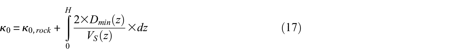
where κ_0,rock is the κ₀ for the underlying rock half-space (0.006 s), and H and z are the profile thickness and depth, respectively.

Figure 15.

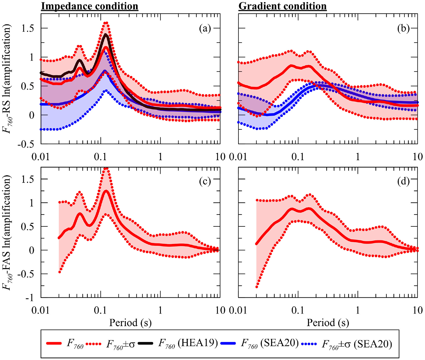
F₇₆₀ factors for impedance and gradient conditions along with those from and Stewart et al. (2020) and F₇₆₀-impedance from HEA19 for linear response spectrum ln(amplification) (a and b). F₇₆₀ factors compute from linear Fourier amplitude spectrum ln(amplification) are given in (a) and (c).

Figure 15(a) and (b) compares F₇₆₀ results from this study with those used in the NSHM for impedance and gradient profiles. At impedance sites, larger F₇₆₀ values are obtained for T_OSC ≤ 0.4 s from this study and from HEA19 than those provided in SEA20, which is attributed to 83% of the simulations in this study utilizing profiles with κ₀ < 0.01 s. A similar trend is observed for the gradient sites, and here, approximately 70% of the profiles have κ₀ < 0.01 s. For mid-to-long periods (T_OSC > 0.4 s), all F₇₆₀ factors seem to converge due to limited soil-damping effects in this period range.

F₇₆₀ obtained from the mean of the linear FAS amplification at sites with 700 m/s ≤ V_S30 ≤ 800 m/s is presented in Figure 15(c) and (d). The FAS amplifications at short periods (high frequencies) decrease with decreasing period more strongly than is seen in RS amplifications, which is an expected consequence of oscillator response characteristics.

Residuals and dispersion analyses

To check the adequacy of the models developed in this work, residuals were computed as the differences of the natural log of computed amplifications (for each considered profile and combination of other dynamic soil properties) and model median prediction. In this section, the residuals are evaluated to check for bias and dispersion characteristics.

Figure 16 shows residuals for three major classes of models for linear simulations plotted as functions of V_S30 and T_OSC/T_nat: V_S30-scaling L1, combined V_S30-scaling and T_nat L5, and T_nat-only L6. For T_OSC of 0.1 s, the averages of L5 and L6 models’ residuals in equally log-spaced V_S30 and T_OSC/T_nat bins exhibit analogous trends and are aligned with the zero line for 100 m/s < V_S30 < 1000 m/s and for T_OSC/T_nat < 1.0. On the contrary, residuals of the V_S30-only L1 model when averaged in T_OSC/T_nat bins (Figure 16(c)) diverge from zero, highlighting the importance of T_nat in influencing simulated site responses at short periods. Comparing long-period residuals of the L5 and L6 models binned with respect to T_OSC/T_nat, averaged L6 residuals are greater than zero for V_S30 < 300 m/s (Figure 16(b)) whereas L5 residuals do not, which indicates the value of including V_S30 into the model form.

Figure 16.

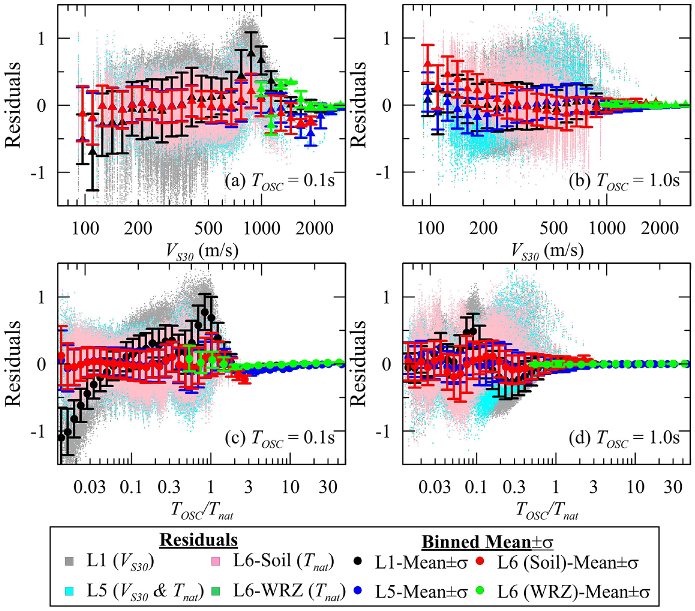
The residuals of L1 (V_S30), L5 (V_S30 and T_nat), L6-Soil (T_nat), and L6-weathered rock zone (T_nat) models along with their binned mean∓σ in V_S30 and T_OSC/T_nat spaces for T_OSC of 0.1 s (a and c) and 1.0 s (b and d).

Next, the dispersion of the residuals is evaluated. Probabilistic seismic hazard analysis (PSHA) considers two types of dispersion in their formulation (McGuire, 2004; Rodriguez et al., 2014; Stafford, 2015): (1) aleatory variability, defined as the inherent randomness of a phenomenon, which cannot be reduced with additional data, and (2) epistemic uncertainty that results from the lack of knowledge and can be diminished through supplementary information. The dispersion of residuals is considered to be a combination of aleatory and epistemic because the V_S profile uncertainty would be dramatically reduced if a site-specific profile was available (hence, it is epistemic), whereas the remaining variability related to motion-to-motion variability and variability in other dynamic properties is arguably mainly aleatory. Since it is a combination of uncertainty and variability, the residual dispersion is subsequently referred to simply as uncertainty.

The uncertainty in this study is represented by standard deviation (σ) relationships, which are computed from the dispersion of residuals. Figure 17(a) shows σ for linear RS L1, L5, L5 (HEA19), and L6 models as a function of T_OSC. Figure 17(b) similarly shows σ for total RS amplification functions L5 + N2 and L5 + N2 (HEA19). The comparison of the model residuals indicates that

• The L5 function given as the summation of f(V_S30) in Equation 4 and f(T_nat)_L5 in Equation 5 results in an ∼11% reduction in σ relative to the L5 model from HEA19.

• Values of σ for f(T_nat)_L6-Soil are similar to those for the L5 model except that the former is slightly larger than the latter for 0.2  < T_OSC < ∼0.9 s. This indicates that a combined V_S30 and T_nat model (L5) performed better than one conditioned on T_nat alone (L6).

• L5 + N2 produces lower σ values relative to L5 + N2 (HEA19) for T_OSC ≥ 1.0 s. This is a result of improvements in the f(T_nat) term.

Figure 17.

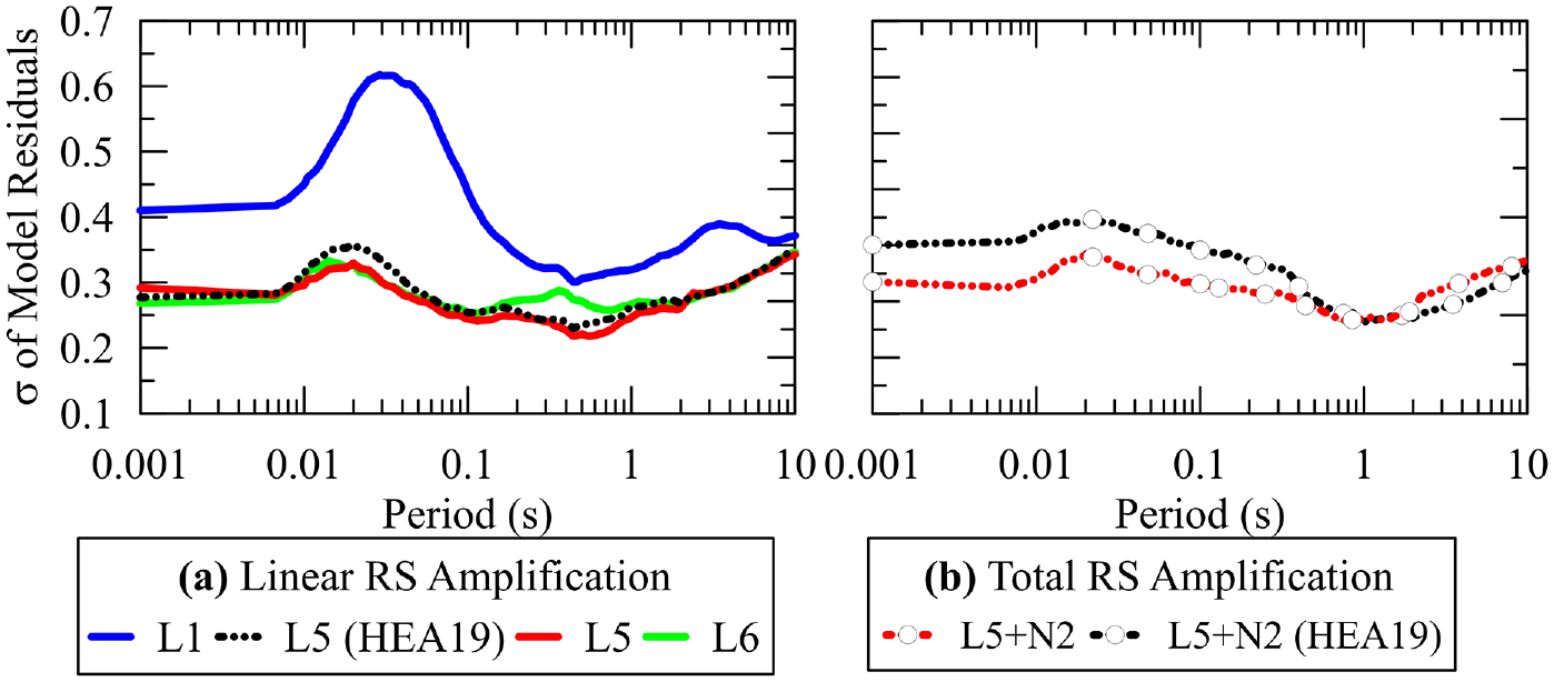
Standard deviation (σ) of (a) linear L1 and L5 (HEA19) calculated using Harmon et al. (2019b) coefficients, L5 and L6 models, and (b) total L5 + N2 and L5 + N2 (HEA19) models as function of T_OSC.

Figure 18(a) and (b) presents the σ of L1 and L5 residuals, respectively. For the F_lin model, the trends in σ are described as,

$${\sigma }_{\mathrm{Flin}}=\{\begin{array}{c}{u}_1·\ln (V_{l1}/V_{l2})+u_2\hfill \\ u_1·\ln (V_{S30}/V_{l2})+u_2\hfill \\ u_2\hfill \end{array}\begin{array}{c}{V}_{S30}<V_{l1}\hfill \\ V_{l1}\le V_{S30}\le V_{l2}\hfill \\ V_{S30}>V_{l2}\hfill \end{array}$$

(18)

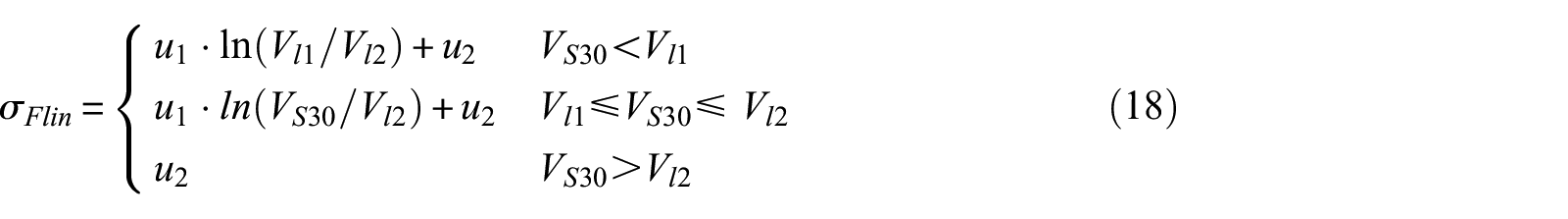
where u₁ and u₂ are period-dependent coefficients; V_l1 is the limiting velocity below which σ is constant; and V_l2 is the limiting velocity beyond which σ is equal to u₂. The proposed σ relationships for the L1 and L5 FAS models are presented in Figure B.37. For median L6 RS and FAS soil amplification models, the same function in Equation 17 is utilized, but V_l1, V_l2, and V_S30 are replaced with T₁, T₂, and T_nat, respectively (Figure 18(d)). Moreover, a power relationship ( $\sigma =u_3\times {[f/f_{\mathrm{nat}}]}^{u_4}$ ) is adopted to model σ for the L6 RS WRZ amplification, as illustrated in Figure 18(e).

Figure 18.

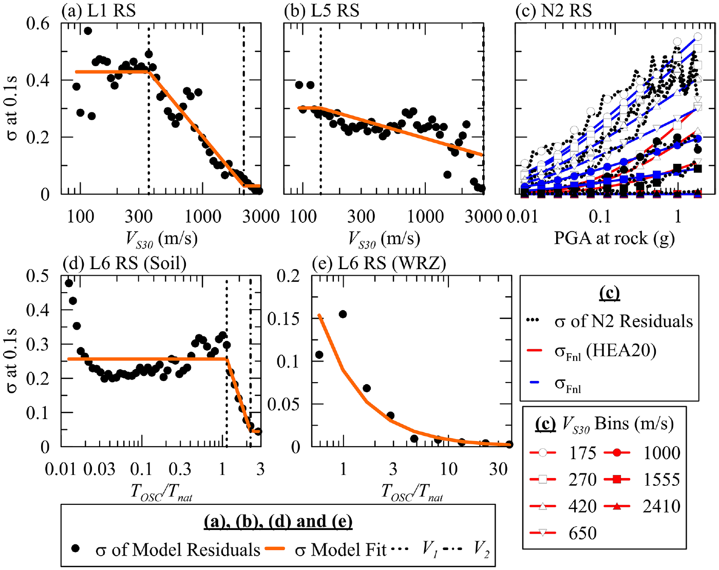
Standard deviation (σ) model estimations for (a) L1, (b) L5, (d) L6 RS (Soil), and (e) L6 RS (weathered rock zone) median site amplification functions along with σ of all these models’ residuals, and (c) σ of N2 RS model residuals as a function of V_S30 and PGA at rock and estimations from newly proposed σ model and HEA20 for T_OSC of 0.1 s. RS: response spectrum.

For the NL components of amplification, a prior model Hashash et al. (2020b) (HEA20) is updated due to the following concerns:

1. HEA20 significantly underestimates the σ from the residuals of N2 model as functions of V_S30 and PGA_r such that σ values from HEA20 for V_S30 ≤ 650 m/s are significantly lower that those from simulated models’ residuals. (Figure 18(c)).

2. HEA20 produces unreasonably low σ (around 0.3) for low V_S30 sites (175 m/s) and high PGA values (>0.5 s), where larger σ values (on the order of ∼0.65) from the simulations are observed (Figure 18(c)).

Accordingly, a new σ function is suggested for the NL model,

$${\sigma }_{\mathrm{Fnl}}={\sigma }_{f2}·\ln \left(\frac{\mathrm{PG}{A}_r+{\sigma }_f}{{\sigma }_f}\right)$$

(19)

where σ_f is a period-dependent coefficient, and σ_f2 is given as:

$${\sigma }_{f2}=\{\begin{array}{c}{\sigma }_c\hfill \\ \left[\frac{-{\sigma }_c}{\ln \left(\frac{V_{n2}}{V_{n1}}\right)}\right]·\ln \left(\frac{V_{S30}}{V_{n1}}\right)+{\sigma }_c\hfill \\ 0\hfill \end{array}\begin{array}{c}\begin{array}{c}{V}_{S30}<V_{n1}\hfill \end{array}\hfill \\ \multicolumn{1}{c}{\begin{array}{c}{V}_{n1}\le V_{S30}<V_{n2}\hfill \end{array}}\\ \multicolumn{1}{c}{V_{S30}\ge V_{n2}}\end{array}$$

(20)

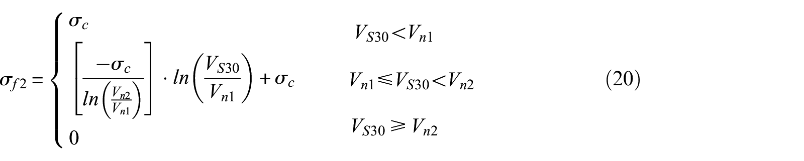
The new σ_Fnl function differs from HEA20 in terms of using V_n1 and V_n2 period-dependent coefficients instead of constant values of 300 and 1000 m/s. Figure 18(c) compares the ${\sigma }_{\mathrm{Fnl}}$ predictions from this study and HEA19 to σ values from N2 model residuals; the results indicate that the dispersion from the present model is more consistent with σ from data.

The two sources of uncertainty are assumed to be independent and can be combined as given in Equation 20 to produce σ for the total amplification ( ${\sigma }_{\mathrm{FS}}$ ).

$${\sigma }_{\mathrm{FS}}=\sqrt{{\sigma }_{\mathrm{Flin}}^2+{\sigma }_{\mathrm{Fnl}}^2}$$

(21)

The influence of ${\sigma }_{\mathrm{Fnl}}$ from Equation 18 and HEA20 on ${\sigma }_{\mathrm{FS}}$ , in which the ${\sigma }_{\mathrm{Flin}}$ is obtained using σ_v of SEA20, is evaluated in Figure 19 for sites with V_S30 of 185 and 250 m/s and PGA_r conditions of 0.65 and 0.95 g. The total amplification ( $F_S$ ) $\mp {\sigma }_{\mathrm{FS}}$ calculated using ${\sigma }_{\mathrm{Fnl}}$ from HEA20 exhibits unexpected contraction for 0.03 s < T_OSC < 0.3 s, which is corrected (increased) in the proposed model.

Figure 19.

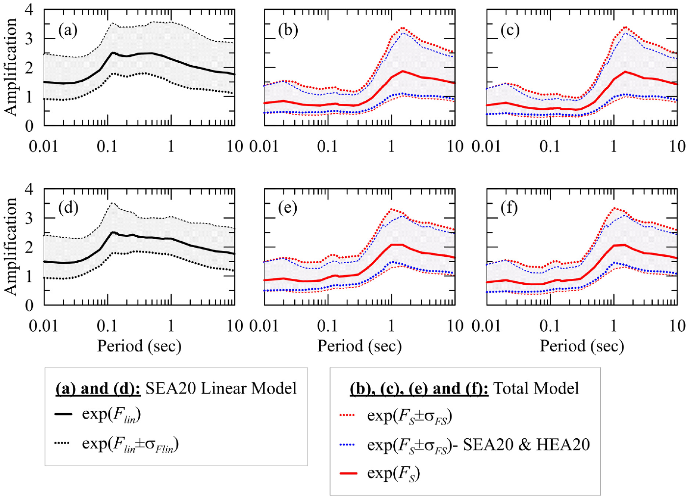
SEA20 linear model ∓1σ_Flin for (a) V_S30 = 185 m/s, (d) V_S30 = 250 m/s, SEA20 linear + HEA20 NL model ∓1σ_FS where σ_Flin from SEA20, and σ_Flin from HEA20 and from this study for (b) V_S30 = 185 m/s and PGA_r = 0.65 g, (c) V_S30 = 185 m/s and PGA_r = 0.95 g, (e) V_S30 = 250 m/s and PGA_r = 0.65 g, and (f) V_S30 = 250 m/s and PGA_r = 0.95 g.

Model limitations and application

The site amplification functions described in this article have limitations that should be considered in potential forward applications. These include

1. Assumptions of 1D site response: The simulated amplification data do not consider multidimensional wave propagation effects that can occur in sedimentary basins.

2. Representative V_S profiles: Even though more than 800 profiles were compiled in HEA19 to produce the representative V_S profiles for each geologic unit in CENA, limited profile data exist for depths (Z) > 100 m. To extend the profiles to larger depths and faster velocities corresponding to weathered and reference rock conditions, V_S is extrapolated to account for the effects of increasing overburden pressure using $\log \left(V_S\right)=n_v\times \log \left(Z\right)+\mathrm{C}$ ; as discussed in Appendix A, the $n_v$ coefficient is constrained from laboratory data and is soil-type dependent. However, other factors may affect the extrapolation such as profiles crossing different geologic horizons of different ages that might increase velocities more rapidly than provided in our model. We are unable to verify the adopted formulation due to limited V_S profile data.

3. Strain level: Results from NL (and EL) SRA with calculated maximum strains greater than 1.0% were excluded during model development. This strain limitation was applied because we are not confident in the estimated shear strengths that were used in model development and wish to exclude results that are strongly influenced by such estimates (i.e. sites where large strains develop). Similar criterion can be given using the strain index, I_y (PGV_r/V_S30) used to predict the peak strain in these analyses (Kim et al., 2016). Figure 20 shows the dependence of I_y on the maximum strains computed in NL analyses; the 1% strain limit applied for NL analyses corresponds to I_y < 0.1%–0.2%, indicating that this I_y range can be accepted as the upper bound of model applicability.

4. Site profile: The use of all V_S30-conditioned RS and FAS models is limited to sites with V_S30 ≥ 180 m/s since profiles with V_S30 < 180 m/s might contain a very soft layer resulting in a large impedance contrast where strain concentrations are expected. Such conditions can produce a “base isolation” behavior that is considered to be unrealistic. Moreover, the depths of site profiles in this study are limited to 1000 m, and thus, the proposed functions likely do not apply for deeper profiles such as in the CP region (Boyd et al., 2022).

Figure 20.

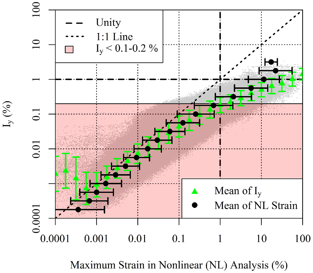
Strain index, I_y, given as a function of maximum strain occurred in each nonlinear analyses along with I_y applicability limit as <0.1%–0.2%.

The L1 function presented above is modular, and the fundamental parameter to utilize these relationships is V_S30. An alternative single-parameter model conditioned solely on T_nat (L6), which reduces uncertainties, is also provided. However, our recommendation is not to use an T_nat-only model but a combined V_S30 and T_nat model (L5), which has improved capabilities for capturing site response over a wide frequency range. For NL models, there is no preference between the models based on PGA_r and SA_r, but modular L_# + N_# is recommended over K models. We provide the multiple models for NL response to enable users to consider model-based epistemic uncertainties if they choose. The RS relationships are applicable for 0.001 s ≤ T_OSC ≤ 10.0 s. For the FAS relationships, this range is defined as 0.1 Hz ≤ f ≤ 33.0 Hz since the maximum frequency content (f_max) is limited to 50.0 Hz, and large scatter of the NL and total FAS amplification data leads to difficulties in the implementation of models for f_OSC > 33.3 Hz (Ilhan, 2020). Both the RS and FAS models developed here provide amplification relative to V_S = 3000 m/s.

The σ relationships share the applicable period / frequency bounds described above. The modular terms (e.g. linear f(T_nat)_L5 or NL N2) or T_nat-based L6 from this study can be combined with linear amplification models from literature (e.g. the ergodic linear SEA20 relationship) as described in the work by Hashash et al. (2021).

Conclusion

This article develops a series of RS and FAS site amplification models for sites in CENA using a database of 3,656,835 1D simulations (1,218,945 each of linear, EL, and NL). The simulation database composed of 148,050 unique generic site profiles is approximately two times larger than the prior data set and incorporates a more comprehensive range of site conditions for model development. The V_S30-scaling L1 relationship deviates from prior V_S30-dependent models—whereas prior models had a decay in short-period amplification as V_S30 decreases for sites with V_S30 < ∼600 m/s, the current models provide flat amplification in this range. The prior L5 (V_S30 and T_nat-dependent) RS models are modified to provide higher-mode amplification at sites with multiple V_S impedance contrasts through a Gaussian term. This improvement reduces model uncertainties modestly (∼11%).

A new T_nat-conditioned L6 RS function is provided to capture resonance effects that are commonly observed in the simulated amplification results. The L6 model produces lower uncertainties than V_S30-scaling model (L1). The uncertainties from L6 are similar to those from a combined V_S30 and T_nat model (L5), which indicates that the influence of T_nat on simulated site amplification is strong and V_S30 values add relatively little additional information. However, it is known from prior empirical studies that V_S30-based models are effective over a wide frequency range, which leads to our recommendation to use coupled V_S30 and T_nat models when practical. For the common case in which empirical models conditioned on V_S30 are used to estimate linear amplification relative to 760 m/s sites, the T_nat-component of the L5 model can be used along with new F₇₆₀ models in applications. The resemblance between the linear RS and FAS amplification is utilized to implement all RS functions for the modeling of FAS amplification. Standard deviation relationships for combined aleatory and epistemic uncertainties for median RS and FAS models are also proposed. Model limitations are described in the previous section.

Supplemental Material

sj-docx-1-eqs-10.1177_87552930231215723 – Supplemental material for Simulated site amplification for Central and Eastern North America: Data set development and amplification models

Supplemental material, sj-docx-1-eqs-10.1177_87552930231215723 for Simulated site amplification for Central and Eastern North America: Data set development and amplification models by Okan Ilhan, Youssef MA Hashash, Jonathan P Stewart, Ellen M Rathje, Sissy Nikolaou and Kenneth W Campbell in Earthquake Spectra

Supplemental Material

sj-xlsx-2-eqs-10.1177_87552930231215723 – Supplemental material for Simulated site amplification for Central and Eastern North America: Data set development and amplification models

Supplemental material, sj-xlsx-2-eqs-10.1177_87552930231215723 for Simulated site amplification for Central and Eastern North America: Data set development and amplification models by Okan Ilhan, Youssef MA Hashash, Jonathan P Stewart, Ellen M Rathje, Sissy Nikolaou and Kenneth W Campbell in Earthquake Spectra

Supplemental Material

sj-xlsx-3-eqs-10.1177_87552930231215723 – Supplemental material for Simulated site amplification for Central and Eastern North America: Data set development and amplification models

Supplemental material, sj-xlsx-3-eqs-10.1177_87552930231215723 for Simulated site amplification for Central and Eastern North America: Data set development and amplification models by Okan Ilhan, Youssef MA Hashash, Jonathan P Stewart, Ellen M Rathje, Sissy Nikolaou and Kenneth W Campbell in Earthquake Spectra

Supplemental Material

sj-xlsx-4-eqs-10.1177_87552930231215723 – Supplemental material for Simulated site amplification for Central and Eastern North America: Data set development and amplification models

Supplemental material, sj-xlsx-4-eqs-10.1177_87552930231215723 for Simulated site amplification for Central and Eastern North America: Data set development and amplification models by Okan Ilhan, Youssef MA Hashash, Jonathan P Stewart, Ellen M Rathje, Sissy Nikolaou and Kenneth W Campbell in Earthquake Spectra

Supplemental Material

sj-xlsx-5-eqs-10.1177_87552930231215723 – Supplemental material for Simulated site amplification for Central and Eastern North America: Data set development and amplification models

Supplemental material, sj-xlsx-5-eqs-10.1177_87552930231215723 for Simulated site amplification for Central and Eastern North America: Data set development and amplification models by Okan Ilhan, Youssef MA Hashash, Jonathan P Stewart, Ellen M Rathje, Sissy Nikolaou and Kenneth W Campbell in Earthquake Spectra

Supplemental Material

sj-xlsx-6-eqs-10.1177_87552930231215723 – Supplemental material for Simulated site amplification for Central and Eastern North America: Data set development and amplification models

Supplemental material, sj-xlsx-6-eqs-10.1177_87552930231215723 for Simulated site amplification for Central and Eastern North America: Data set development and amplification models by Okan Ilhan, Youssef MA Hashash, Jonathan P Stewart, Ellen M Rathje, Sissy Nikolaou and Kenneth W Campbell in Earthquake Spectra