Systematic assessment of nonlinear soil behavior at KiK-net sites in Japan: Thresholds and controlling site factors

Abstract

We address two open questions concerning nonlinear soil behavior in a seismic hazard and risk context; (1) which site proxies can be used to predict and map nonlinear site amplification? (2) At which level of ground-motion intensity should such nonlinear models be considered? To answer these questions, we use the KiK-net network in Japan, which includes stations with instruments at both surface and depth, considering events recorded between 1997 and 2024. Using the surface-to-borehole ratio, we systematically capture the empirical effects of nonlinear soil response as the amplitude change and frequency shift between individual events and the linear site response. We then derive station-specific parameters for degree of nonlinearity and threshold for onset of nonlinear behavior. The statistical correlation between nonlinearity and a selection of geotechnical and geological site parameters shows that although parameters characterizing the depth to bedrock and the shallowest part of the soil layer have a promising potential for capturing nonlinear site amplification, the correlation is generally low, suggesting that a single site parameter is not sufficient. As a consistent reference for ground-motion intensity, we empirically calculate PGA_emp.rock, as an approximation for PGA recorded on a standard outcropping rock site with V_S30 = 760 m/s (average shear-wave velocity of upper 30 m). When analyzing the nonlinear behavior for all recorded events, we define the nonlinear soil behavior as significant when the amplitude change, and frequency shift are greater than 10% for the majority (50%) of the records. We find that in the PGA_emp.rock-range 1−3 m/s² nonlinear soil behavior is significant only for soft soil stations (V_S30 < 250 m/s) with intermediate sediment thickness (<30 m). While, according to the mean behavior of all sites, regardless of grouping, nonlinearity is significant only at PGA_emp.rock > 3 m/s². These results show that for nonlinear site-amplification modeling, the onset of nonlinearity is strongly related to the site conditions.

Introduction

Nonlinear soil behavior occurs during high strain levels due to a degradation of the mechanical properties of the soil and hysteretic behavior with a simultaneous reduction in the shear modulus and an increase in shear-wave damping with increasing levels of strain (e.g. Bonilla et al., 2005; Darendeli, 2001). Such nonlinear site effects are mainly expected for soft soil sites and strong ground shaking. Nonlinear site amplification factors used in ground-motion models (GMMs) are therefore commonly based on site, period and intensity, commonly using a site proxy characterizing the softness of the soil and an intensity measure of the ground shaking on rock (e.g. Borcherdt, 2002; Chiou and Youngs, 2008; Choi and Stewart, 2005; Stewart et al., 2003). Most nonlinear site amplification models are based on the peak ground acceleration (PGA) or spectral acceleration for a given period T (SA(T)), and the average shear-wave velocity in the upper 30 m of the soil column (V_S30) is the most common site proxy (e.g. Choi and Stewart, 2005; Hashash et al., 2020; Sandikkaya et al., 2013; Seyhan and Stewart, 2014). However, recent studies have shown that such nonlinear amplification models may overestimate the nonlinear site response (Bard et al., 2024; Loviknes et al., 2021; Paolucci et al., 2021). Furthermore, it has been suggested that V_S30 is not the optimal proxy for characterizing nonlinearity, particularly when soft surficial layers overlay stiffer material (Bonilla et al., 2011; Ji et al., 2021; Régnier et al., 2013).

When investigating the correlation between nonlinearity and alternative site proxies, studies have mainly focused on site-specific (direct) site parameters, obtained using geotechnical investigations and seismic surveys, with especially the site fundamental frequency of resonance (f₀) and the depth to bedrock (Z_0.8) having potential for characterizing nonlinear site amplification. (Derras et al., 2020; Kwak and Seyhan, 2020; Régnier et al., 2013). However, for seismic hazard and risk models, there is a need to estimate the site effects over larger areas and whole regions, and the site conditions can therefore only be derived indirectly through models and maps (e.g. Bergamo et al., 2022; Thompson et al., 2010; Weatherill et al., 2020). The need for large-scale (indirect) site proxies for regional and global seismic hazard and risk assessments considering linear site effects have received increased focus in recent years (e.g. Bergamo et al., 2023; Crowley et al., 2021; Loviknes et al., 2023). Similarly, in this study we will focus on the potential for using indirect site proxies for nonlinear site amplification predictions on regional and large-scale. Particularly we will focus on alternative inferred proxies, other than the commonly used inferred V_S30.

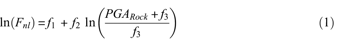
Another central question when dealing with nonlinearity is the ground-motion intensity at which the nonlinear site response starts shifting from linear to nonlinear. Due to the rarity of strong motion recordings with evident nonlinear behavior, these values are often determined using laboratory measurements (e.g. Ciancimino et al., 2023; Vucetic, 1994) and validated for ground motions using simulations and site response models, where linear models are generally considered valid for strains up to 1% and PGA <1 m/s² (e.g. Kaklamanos et al., 2013). Lower nonlinearity thresholds have also been suggested, for example, PGA = 0.5 m/s² (Roten et al., 2009), while Shi and Asimaki (2017) showed that the onset of nonlinearity in terms of PGA varies significantly between stations (0.1–9 m/s²). For nonlinear amplification factors used in GMMs this threshold is typically derived using regression over empirical data and/or simulations that account for soil nonlinearity and V_S30:

$$\ln \left(F_{\mathrm{nl}}\right)=f_1+f_2\ln \left(\frac{\mathrm{PG}{A}_{\mathrm{Rock}}+f_3}{f_3}\right)$$

(1)

where $\ln \left(F_{\mathrm{nl}}\right)$ is the nonlinear amplification factor, PGA_Rock is the median PGA for reference rock, and $f_3$ is the threshold for onset of nonlinearity. For classical GMMs $f_3$ typically ranges between 0.05 and 0.1 g (e.g. Chiou and Youngs, 2008; Choi and Stewart, 2005; Seyhan and Stewart, 2014; Stewart et al., 2003).

With the increase of available ground-motion data, it has also become more common to derive nonlinear site parameters by comparing weak and strong motion (e.g. Bonilla et al., 2011; Castro-Cruz et al., 2020; Noguchi and Sasatani, 2008; Ren et al., 2017; Régnier et al., 2013; Wang et al., 2023). The Kiban–Kyoshin Network (KiK-net, Aoi et al., 2011; Okada et al., 2004) in Japan is particularly useful for studying nonlinear site effects as it has recorded a large number of both weak and strong ground motions and because of its unique configuration with each station having two 3-component accelerometers, one located at the soil surface and the other in a borehole, generally embedded in the bedrock. For KiK-net, studies have found that the average nonlinearity threshold for PGA recorded at the surface is 1 m/s² (Frid and Kamai, 2023; Régnier et al., 2016), but that the threshold varies significantly between stations (Castro-Cruz et al., 2020; Régnier et al., 2013; Wu et al., 2010).

Essentially, in a seismic hazard and risk context, there are two open questions when predicting nonlinear site amplification models for large areas and regions: (1) which site proxies are more suitable for nonlinear site amplification predictions and mapping? (2) At which ground motion intensity do nonlinear site effects become significant?

Studies characterizing the nonlinear soil response at the scale of geotechnical laboratory testing have identified (1) the plasticity index, (2) the grain size of the loose sediments, and (3) the effective pressure acting upon them, as key parameters controlling nonlinear soil behavior (e.g. Darendeli, 2001). To identify site condition indicators that could contribute to characterizing and mapping the susceptibility to nonlinearity, we, therefore, resorted to the velocity profile and site-specific information available at each site, as well as the five following databases available at regional or global scale:

1. 1D velocity Extracted from a 3D Regional Velocity Structure (J-SHIS, www.j-shis.bosai.go.jp).

2. The pedologic database SoilGrid (Poggio et al., 2021).

3. Geomorphological sediment thickness by Pelletier et al. (2016).

4. The Seamless Digital Geological Map of Japan (Geological Survey of Japan, 2015).

5. Engineering Geomorphologic Unit from Wakamatsu and Matsuoka (2013).

Taking advantage of the large and openly available KiK-net strong motion data set, we quantify the nonlinear soil behavior in a systematic manner to estimate both station-specific, but also event-specific nonlinear soil behavior. We follow the method of Régnier et al. (2013), which has been shown to be robust (e.g. Ren et al., 2017), to measure the amplitude change and frequency shift typical for nonlinear soil behavior. We use an updated database containing ground motions recorded by KiK-net from 1997 until the first week of 2024, including the recent M_w7.5 Noto earthquake (Fujii and Satake, 2024).

In the first step, in section “Quantifying nonlinearity for each event,” we use the surface-to-borehole spectral ratios (SBr) of each station, and measure the change in amplitude and shift in frequency of each ground motion relative to the linear site response. Second, in section “Site-specific parameters describing nonlinearity,” site-specific parameters for nonlinear soil behavior are derived using a hyperbolic function fit over the amplitude change and frequency shift estimates for all the recorded events by each considered station. Finally, using the method developed in section “Correlation between nonlinearity and site parameters,” the behavior of the event- and site-specific nonlinearity is explored, both in relation to increasing ground-motion intensity and to the selected geotechnical and geological indicators, as described in the “Results” section.

Data set

Strong-motion records from 1997 to 2024

The Japanese KiK-net (Aoi et al., 2011; Okada et al., 2004) from the National Research Institute for Earth Science and Disaster Resilience (NIED) (2019) is well suited for studies of site-effects as it is a nationwide network with more than 600 sites and instruments at both the surface and in a borehole at depth. In this study, we only consider the 350 stations (Figure 1a) which have recorded more than one event with PGA recorded at surface ≥ 0.5 m/s², shear wave velocity at borehole V_S,B ≥ 760 m/s and at least 10 linear event recordings with PGA_S ≤ 0.1 m/s². From these stations, we use the 115 218 ground motions from the 11 358 events recorded between October 1997 and January 2024 (including the January 1st M_w7.5 Noto earthquake) with magnitude above 3, hypocentral distance below 500 km, PGA_S ≥ 0.01 m/s², signal-to-noise ratio (SNR) above 3 and usable frequency band corresponding to at least 60% of the possible frequency range (0.01–30 Hz). The SNR is calculated using either the pre-event noise, if at least 15 s are available, or the last 20 s of the time window. To further assess the quality of the time series, the ratio of the energy of the expected P- and S-wave window relative to the energy of the entire record, is calculated and only the record where 80% of the energy is within the expected P- and S-wave window is kept. The expected P- and S-wave window duration are calculated as in Perron et al. (2018). The distribution of the PGA recorded at surface of the selected records with hypocentral distance and magnitude are shown in Figure 1b.

Figure 1.

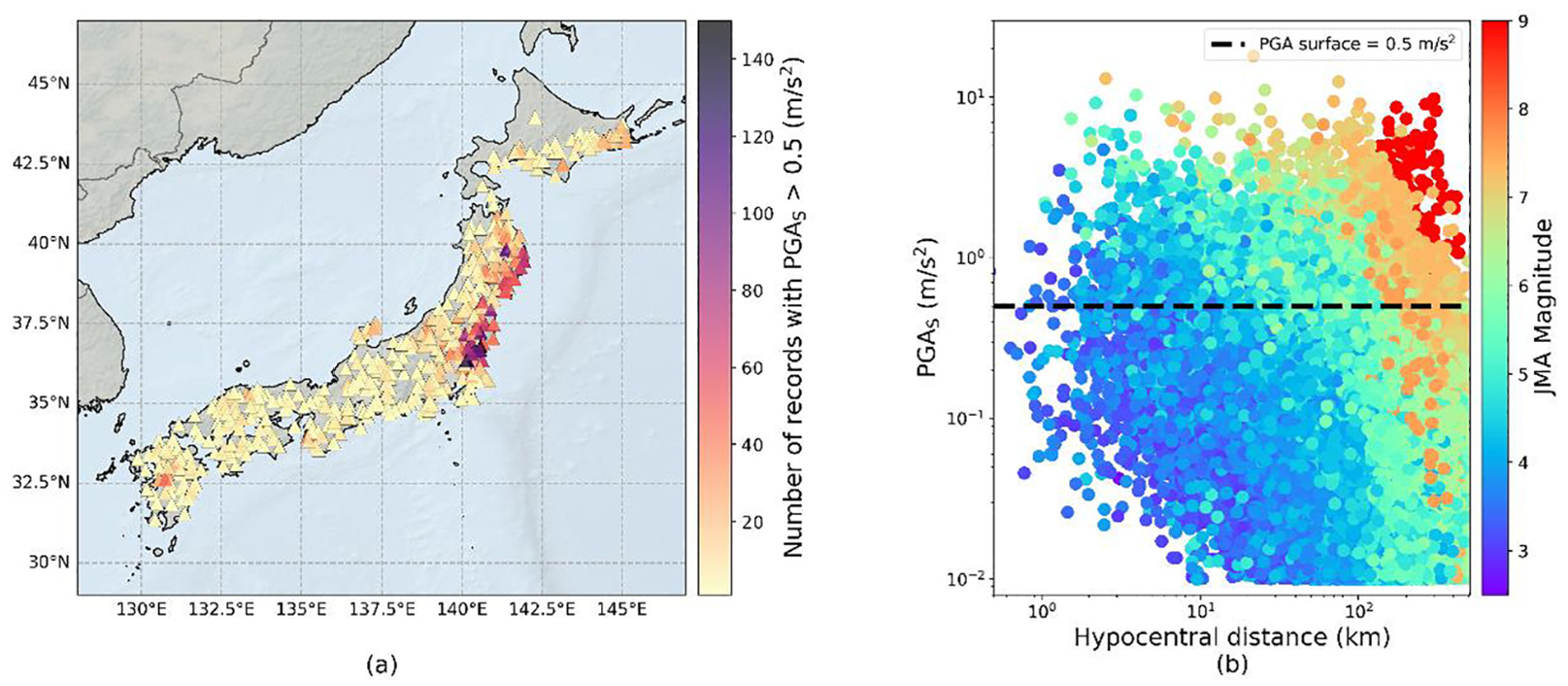
(a) The location of the KiK-NET stations with more than one recorded strong-motion event (PGA_S > 0.5 m/s²), colored by number of recorded strong-motion events. (b) The distribution of PGA (recorded at surface) and hypocentral distance colored by magnitude of the 115 218 records used to measure the nonlinear soil behavior.

Before calculating the Fourier Amplitude Spectras (FAS), the real P- and S-wave arrivals are automatically detected using the short-term average (STA) and long-term average (LTA) technique of Akazawa (2004). The baseline correction is applied by fitting a polynomial to the displacement time series and subtracting the second derivative of the polynomial from the acceleration time series as in Ancheta et al. (2014). Finally, the Fourier Amplitude Spectra are smoothed using a Parzen window of 0.2 Hz.

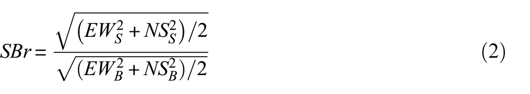
The ground-motion site response can be derived as the standard spectral ratio (SSR) between a site and a rock reference (Borcherdt, 1970). Here, we use the borehole station at each site as the rock reference and derive the site response as the surface-to-borehole ratio (SBr) of the geometric mean of the two horizontal components East-West (EW) and North-South (NS) for Surface S and borehole B:

$$\mathrm{SBr}=\frac{\sqrt{({\mathrm{EW}}_S^2+{\mathrm{NS}}_S^2)/2}}{\sqrt{({\mathrm{EW}}_B^2+{\mathrm{NS}}_B^2)/2}}$$

(2)

A well-known limitation of using a borehole station as reference is the potential for resonances to arise from destructive interference between the upgoing and downgoing waves (Bonilla et al., 2002; Cadet et al., 2012; Parolai et al., 2009, 2012; Şafak, 1995, 1997; Steidl et al., 1996; Tao and Rathje, 2019). Although there exists several methods to identify and correct for such pseudo-resonances and depth effects (e.g. Cadet et al., 2012; Tao and Rathje, 2019), when comparing SBRs (for 166 KiK-net stations) with amplification functions from empirical spectral modeling, Bergamo et al. (2021) have shown that such corrections do not fully comply with the overall set of empirical data. Bergamo et al. (2021) argue that such effects, while relevant for individual cases, may not be systematically significant due to a non-perfectly vertical SH wave propagation; furthermore, the proposed correction factors effects (Cadet et al., 2012) rely on the V_s profile between surface and borehole stations, which might not be reliable for all KiK-net stations (e.g. Poggi et al., 2012, 2013). Furthermore, unlike Cadet et al. (2012) and Bergamo et al. (2021), this study does not aim to retrieve the amplification function with respect to a standard rock outcrop. Instead, it seeks to quantify the change in the site response (captured by the SBr) with increasing ground motions. As the potential depth effects are expected for both the linear and nonlinear responses, it is therefore unlikely that they introduce a bias in our results. Similarly, considering the potential for pseudo-resonances to influence the estimation of frequency shifts, the high correlation between f₀ selected from SBr and horizontal-to-vertical-standard-ratio (HVSR) (selected by Zhu et al., 2021) shown in Figure 2f, further suggests that our results accurately capture the ground resonance frequency (and not a pseudo-resonance due to the destructive interference between up- and downgoing waves). In this study, we thus assume that depth effects can be disregarded when analyzing the degree of nonlinearity, as it has also been assumed by other studies (Castro-Cruz et al., 2020; Régnier et al., 2013, 2016).

Figure 2.

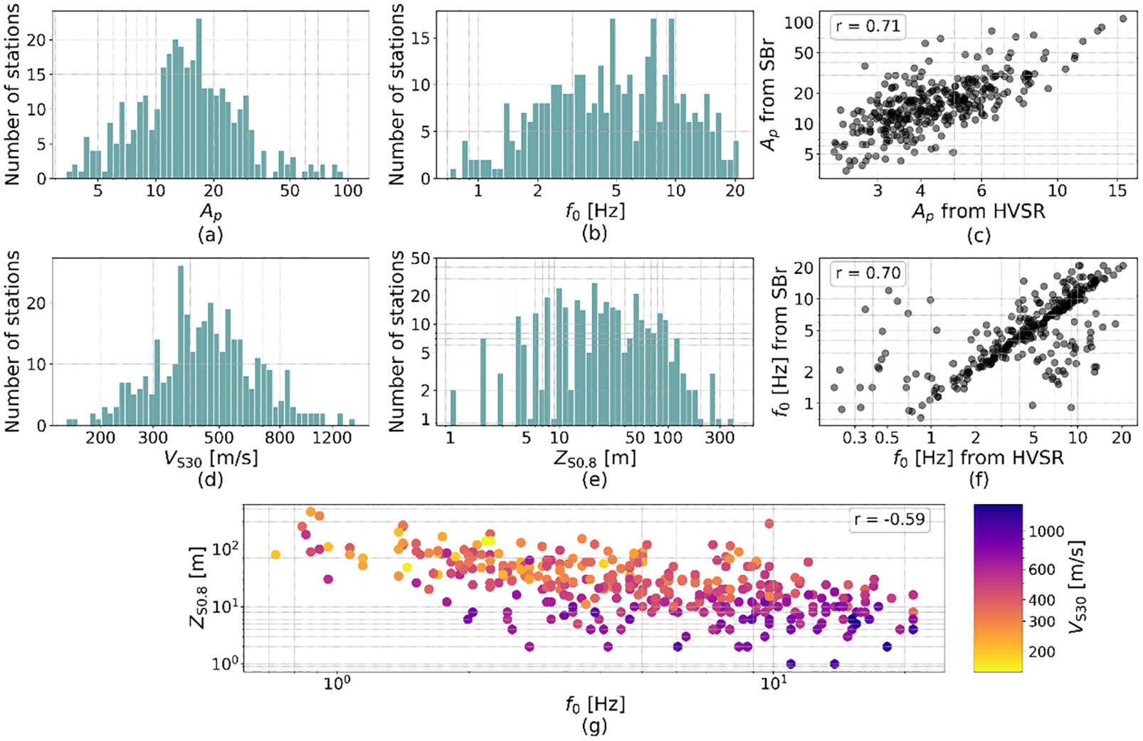
The distribution of the direct site proxies (a) the amplitude A_p of the largest peak of the linear site response, (b) the fundamental frequency f₀, (d) V_S30, and (e) depth to S-wave velocity 0.8 km/s (Z_S0.8, y-axis in log-scale). (c) The peak amplitude (A_p), and (f) fundamental frequency (f₀) extracted from the site-averaged linear surface-to-borehole ratio (SBr) compared to the same values extracted from station horizontal-to-vertical-standard-ratio (HVSR) by Zhu et al. (2021), and (g) the relation between fundamental frequency f₀ and depth to S-wave velocity 0.8 km/s (Z_S0.8) colored by V_S30.

Site condition parameters from in situ geophysical measurements

From the linear site response

We extract the fundamental resonance frequency (f₀) and amplitude of the largest peak (A_p) from the linear surface-to-borehole transfer function (SBr) for each station. The station specific linear SBr is derived as the mean of all events with PGA_S ≤ 0.1 m/s². The peaks used to select the amplitude and fundamental frequency (from the first peak) are found using the height and prominence criteria from Zhu et al. (2021). The station distributions of f₀ and A_p are shown in Figure 2a and b, respectively. Because the resonance frequency extracted from SBr can be influenced by depth effects at the borehole (e.g. Cadet et al., 2012), as also described in the previous section, we compare our resonance frequency and peak amplitude with those selected from HVSR by Zhu et al. (2021) (Figure 2c and f). The correlation between the two different sets of values is calculated using the Pearson correlation (r) coefficient and shows a high correlation (r = 0.7), for both sets of values. Since the amplitude peak and fundamental frequency are selected from an expanded data set and thus available for more stations, we therefore chose to use the maximum amplitude and fundamental frequencies extracted from the SBrs in this study. Although f₀ and A_p are here derived from earthquake data and therefore cannot specifically be considered site proxies, the lack of available H/V noise measurements for KiK-net sites makes such values the only available option for estimating f₀ and A_p. Furthermore, several similar studies have considered f₀ and A_p estimated from earthquake data as predictors for site amplification (e.g. Derras et al., 2017; Zhu et al., 2022).

Velocity profiles

A great advantage of the KiK-net network is the availability of 1D velocity profiles measured at each station between the surface and borehole receiver (National Research Institute for Earth Science and Disaster Resilience (NIED) 2019). In this study, we use the values computed by Zhu et al. (2021) as the time-averaged velocity for the selected depths above the borehole for KiK-net stations. We focus on the classical V_S30 and the depth to S-wave velocity 0.8 km/s; Z_S0.8, which both are site parameters used in the recent European building code (Eurocode 8) to classify soil types (e.g. Paolucci et al., 2021). The relation between f₀, Z_S0.8 and V_S30 is given in Figure 2g, showing that the absolute correlation between f₀ and Z_S0.8 is high (|r| = 0.59) with low fundamental frequency generally corresponding to deep Z_S0.8 and high V_S30. The station distribution is shown in Figure 2d and e.

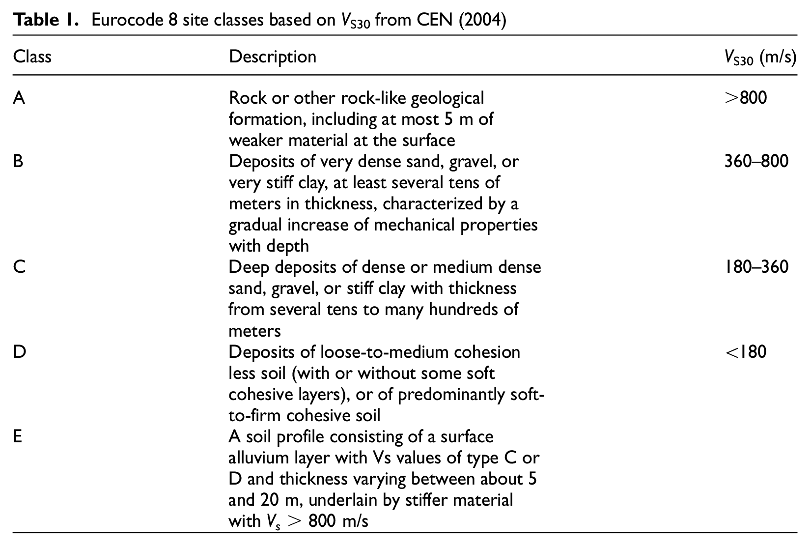
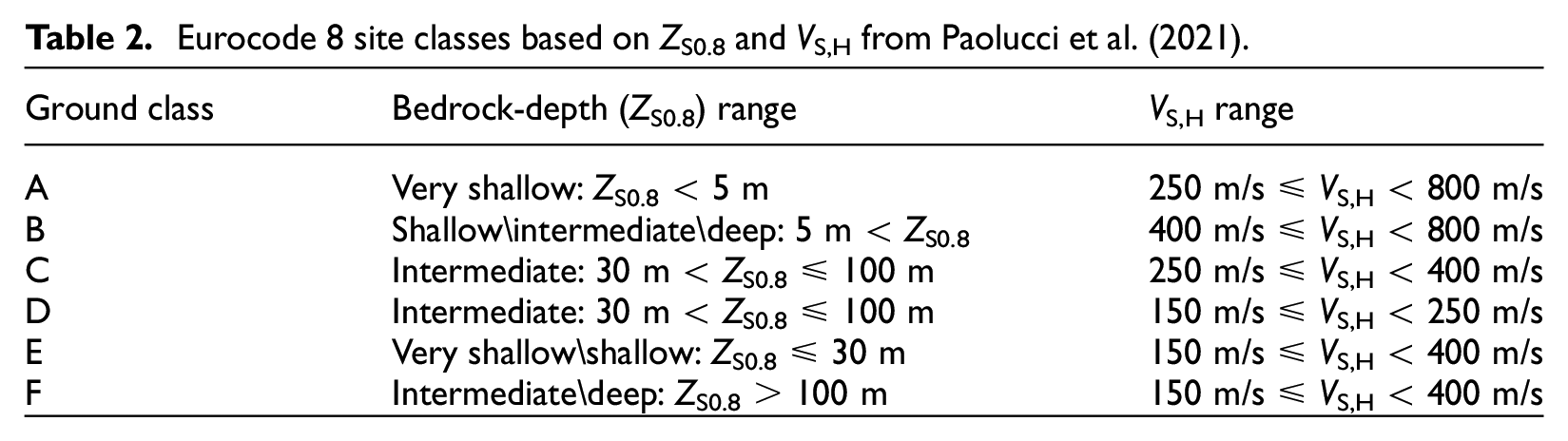
Eurocode 8 soil classes

Seismic building codes aim to ensure that structures are able to resist the ground shaking during an earthquake. To deal with site effects, seismic building codes provide amplification factors based on different soil classes. For Europe, these site classes are defined by the Eurocode 8 (EC8, CEN, 2004) with the geophysical criterion involving different V_S30 ranges for classes A–D and includes Z_S0.8 only for class E. A new site classification has recently been proposed (Paolucci et al., 2021), based on Z_S0.8 and V_S,H (depth-averaged V_S of the sediments for Z_S0.8 < 30 m and V_S,H = V_S30 for Z_S0.8 > 30 m). Here, we use both the old EC8 site classes (from hereon called EC8-1), as well as from the new Eurocode 8 draft (EC8-draft). The grouping criteria for EC8-1 and EC8-draft are given in Tables 1 and 2, respectively, and the station distributions are shown in Figure 3e and f.

Table 1.

Eurocode 8 site classes based on V_S30 from CEN (2004)

Class	Description	V S30 (m/s)
A	Rock or other rock-like geological formation, including at most 5 m of weaker material at the surface	>800
B	Deposits of very dense sand, gravel, or very stiff clay, at least several tens of meters in thickness, characterized by a gradual increase of mechanical properties with depth	360–800
C	Deep deposits of dense or medium dense sand, gravel, or stiff clay with thickness from several tens to many hundreds of meters	180–360
D	Deposits of loose-to-medium cohesion less soil (with or without some soft cohesive layers), or of predominantly soft-to-firm cohesive soil	<180
E	A soil profile consisting of a surface alluvium layer with Vs values of type C or D and thickness varying between about 5 and 20 m, underlain by stiffer material with Vs > 800 m/s

Table 2.

Eurocode 8 site classes based on Z_S0.8 and V_S,H from Paolucci et al. (2021).

Ground class	Bedrock-depth (ZS0.8) range	V S,H range
A	Very shallow: ZS0.8 < 5 m	250 m/s ≤ VS,H < 800 m/s
B	Shallow\intermediate\deep: 5 m < ZS0.8	400 m/s ≤ VS,H < 800 m/s
C	Intermediate: 30 m < ZS0.8 ≤ 100 m	250 m/s ≤ VS,H < 400 m/s
D	Intermediate: 30 m < ZS0.8 ≤ 100 m	150 m/s ≤ VS,H < 250 m/s
E	Very shallow\shallow: ZS0.8 ≤ 30 m	150 m/s ≤ VS,H < 400 m/s
F	Intermediate\deep: ZS0.8 > 100 m	150 m/s ≤ VS,H < 400 m/s

Figure 3.

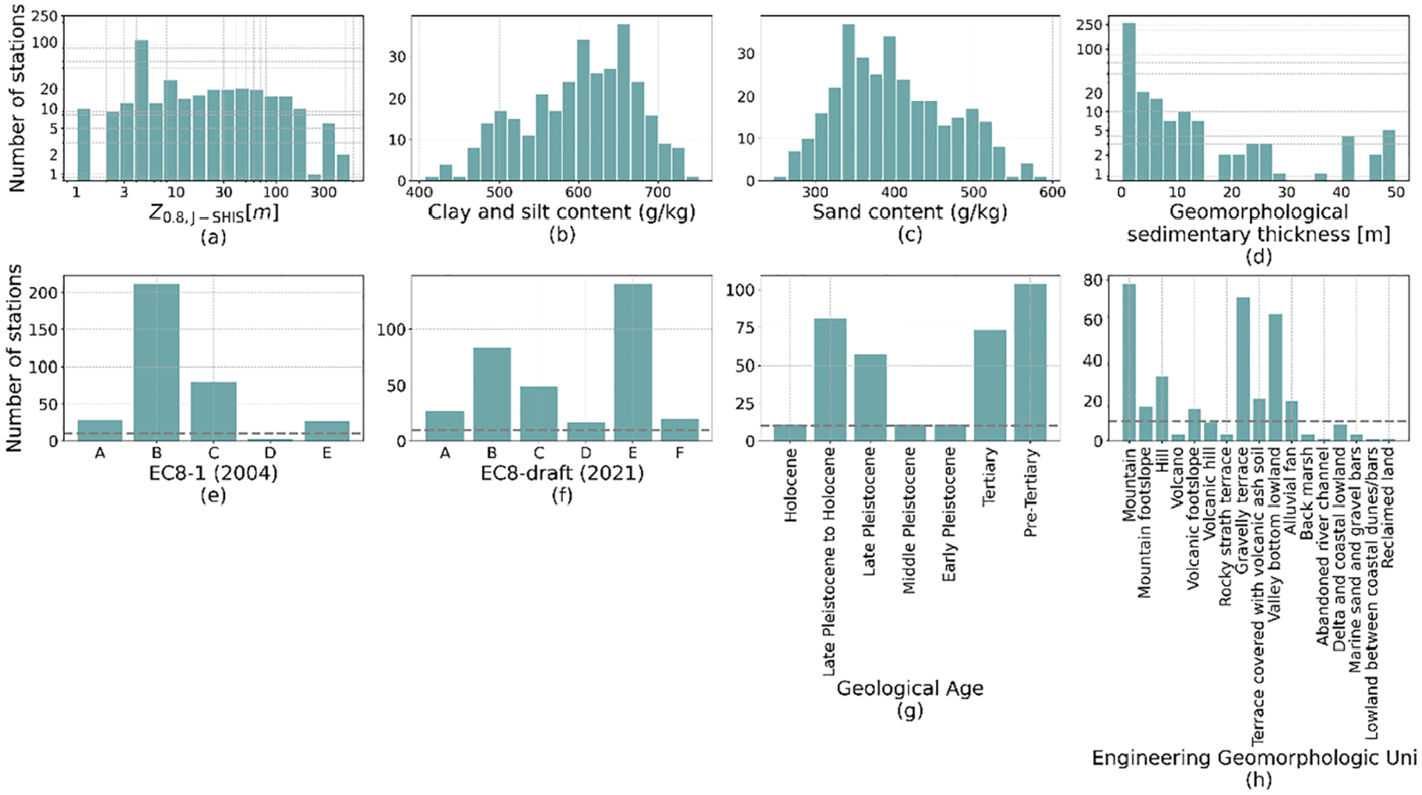
The distribution of the indirect continuous site-proxies (a) depth to S-wave velocity 0.8 km/s Z_0.8,J−SHIS derived from the 1D Model Extracted from a 3D Regional Velocity Structure (J-SHIS), (b) Clay and Silt content and (c) Sand content derived from SoilGrid, (d) Geomorphological sedimentary thickness by Pelletier et al. (2016), and the distribution of the categorical site-proxies (e) Eurocode 8 (EC8-1) soil classes based on V_S30, (f) new Eurocode 8 soil classes (EC8-draft) based on Z_S0.8 and V_S,H (g) geological age, and (h) Engineering Geomorphological Unit. The y-axis for Z_0.8,J−SHIS (a) and Geomorphological sedimentary thickness (d) are in log-scale.

Indirect site proxies

J-SHIS

The 3D Regional Velocity Structure of the Japan Seismic Hazard Information Station (J-SHIS, www.j-shis.bosai.go.jp), consists of several layers with constant material properties, including S-wave velocity. Here, we only consider the 9th layer (Z_0.8,J−SHIS), corresponding to depth to V_S = 0.8 km/s, as provided in the Zhu et al. (2021) site database. The station distribution of Z_0.8,J−SHIS is shown in Figure 3a, and the relation between Z_0.8,J−SHIS and the directly measured V_S30 and Z_S0.8 are shown in Figure S1a and e in Supplementary Material. The correlation between Z_0.8,J−SHIS and the directly measured parameters are low (|r| < 0.4), which has also been observed in previous studies (Zhu et al., 2019).

SoilGrid

The SoilGrid database is a globally gridded map of pedological properties predicted using machine learning with observed soil profiles and environmental covariate data as input (Poggio et al., 2021). The database consists of predicted pedological properties at 250 m resolution for six depth levels from the top surface down to 2 m. Previous studies have shown the correlation between inferred pedological parameters from the SoilGrid database and site condition parameters (V_S30, Z_S0.8), as well as the local earthquake response (Bergamo et al., 2019, 2022).

Because the content of silt, clay, and sand at a site are strongly related to the plasticity index (e.g. Ciancimino et al., 2023), and the plasticity index is an indicator for nonlinearity in geotechnical tests (Vucetic and Dobry, 1991), we focus, in this study, on the weight fractions of silt, clay, and sand (g/kg). We use the values predicted for a depth range of 1–2 m, which is both the deepest available layer and the depth layer shown to have the best correlation with geophysical site condition proxies (V_S30) in Bergamo et al. (2019). The distributions of these layers are shown in Figure 3b and c, and the correlation between the SoilGrid layers and V_S30 and Z_S0.8 are shown in Figure S1b-d and g-i in Supplementary Material.

Geomorphological sediment thickness

Pelletier et al. (2016) used DEM and geological maps to distinguish between the different landforms; lowlands, uplands, hillslopes, and valley bottoms. For each landform, the thickness of sediments, soil, and intact regolith is then inferred using several globally and regionally available values including geological maps, water table depth, and climate data. The final model provides a global map of inferred regolith, soil, and sediment thickness down to 50 m. Although this model was originally developed for land surface modeling, it has been shown to be a statistically significant predictor of local earthquake response (Loviknes et al., 2023). When compared to V_S30 and Z_S0.8, the Geomorphological sediment thickness shows higher values for low V_S30 and an increase with Z_S0.8 (Figure S1d and h in Supplementary Material). The distribution of this parameter over the KiK-net station population is shown in Figure 3d.

Engineering geomorphologic unit

We use the engineering geormorphological classification developed by Wakamatsu and Matsuoka (2013). The Wakamatsu and Matsuoka (2013) engineering geormorphological units was collected from the 7.5-arc-second “Japan Engineering Geomorphologic Classification Map (JEGM)” and based on engineering-based geomorphologic classification standards. The sites are separated into 24 geomorphological classes, but as shown in the station distribution in Figure 3g, the classes Reclaimed land, Lowland between coastal dunes and/or bars and Abandoned river channel only includes one station each and are therefore not included in the further analysis of this study. In addition, no station is classified under the classes, Natural levee, Sand dune, Filled land, Rock shore, rock reef, Dry riverbed, Riverbed and Water body. In the end, therefore, 14 of the engineering geomorphologic classes are considered.

Seamless digital geological map of Japan

Geological information is derived from the Seamless Digital Geological Map of Japan (SDGM, Geological Survey of Japan, 2015). The map has a 1:200,000 resolution and was derived by merging geologic quadrangle maps covering all of Japan. In this study, we consider the geological age from the SDGM that is provided in the Zhu et al. (2021) site database, however with the Tertiary ages grouped together and ages older than Tertiary grouped as pre-Tertiary. The station distribution is shown in Figure 3h.

Method

Quantifying nonlinearity for each event

Nonlinearity is mainly identified in the site response as a decrease in site amplification at frequencies higher than the fundamental frequency of resonance and a shift of the latter to lower frequencies. Here, we aim to systematically measure and quantify these two effects in the site response transfer function obtained from the SBr.

We follow the method of Régnier et al. (2013), where the change of amplitude (Amplitude Change Index, ACI) and the shift in frequency (Sh) are measured relative to the linear site response (SBr_lin), as illustrated in Figure 4 for the station FKSH12 for a weak (linear) event (Figure 4a) and a strong (nonlinear) event (Figure 4b). The linear SBr of each site is derived as the mean of all weak events with PGA_S < 0.1 m/s². The same type of measurements for a second example station is shown in Figure S2 in Supplement Material.

Figure 4.

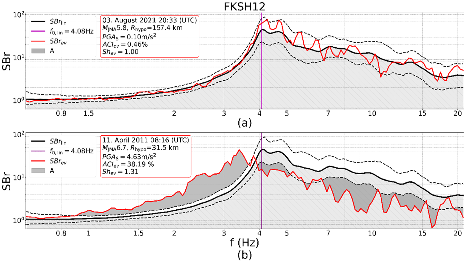
The mean linear surface-to-borehole ratio (SBr_lin, black solid line) with 95% and 5% quantile ( ${\mathrm{SBr}}_{\mathrm{lin}}^{\pm }$ , black dashed line) for the station FKSH12 (V_S30 = 449 m/s and Z_S0.8 = 22 m), with the SBr of (a) a weak event (red line) recorded on 3 August 2021 at hypocentral distance R_hypo = 157.4 km as indicated in the red box, and (b) a strong-motion event (red line) recorded on 11 April 2011 at hypocentral distance R_hypo = 31.5 km. The mean linear SBr is here based on 1064 events with PGA_S < 0.1 m/s².

ACI, called the percentage of nonlinearity (PNL) by Régnier et al. (2013), is measured for each event ev as the area between the event-specific SBr (SBr_ev) and the outer limits of SBr_lin, here defined as the 95% ( ${\mathrm{SBr}}_{\mathrm{lin}}^{+}$ ) and 5% quantile ( ${\mathrm{SBr}}_{\mathrm{lin}}^{+}$ ) of the weak SBrs. Finally, ACI is normalized by dividing by the integral of SBr_lin, which makes it more robust to high amplitude weak motions (Wang et al., 2023), and expressed as a percentage (Equations 5 and 6 in Régnier et al., 2013):

$$A=\sum _i^N\{\begin{array}{cc}\left[SB{r}_{lin}^{-}\left(i\right)-SBr\left(i\right)\right]lo{g}_{10}\left(\frac{f_{i+1}}{f_i}\right),for& SBr\left(i\right)\ge SB{r}_{lin}^{+}\\ \left[SB{r}_{lin}^{-}\left(i\right)-SBr\left(i\right)\right]lo{g}_{10}\left(\frac{f_{i+1}}{f_i}\right),for& SBr\left(i\right)\le SB{r}_{lin}^{-}\end{array}$$

(3)

$$\mathrm{AC}{I}_{\mathrm{ev}}=100\frac{A}{\sum _i^N\left|\mathrm{SB}{r}_{\mathrm{lin}}\right|{\log }_{10}\left(\frac{f_{i+1}}{f_i}\right)}$$

(4)

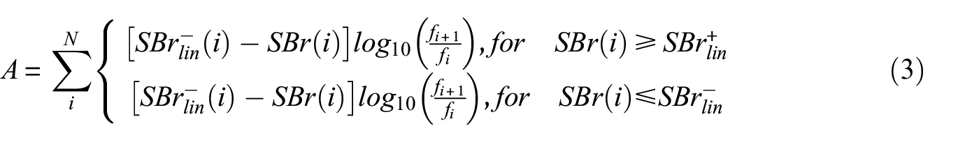
where f_i is the frequency at vector index i in the frequency range 0.6 to 21 Hz. To even out the measurements from high and low frequencies, the frequency vector follows a logarithmic progression interval.

The shift in frequency (Sh) is, as in Régnier et al. (2013), obtained by cross-correlating the event specific SBr_ev and the mean linear SBr_lin, both with frequency vectors in logarithmic scale. Because we assume that the cross-correlation is dominated by the fundamental resonance frequency, the horizontal shift (in log-scale), where the cross-correlation function is maximum, corresponds to the ratio between the linear peak frequency (f_0,lin, purple vertical lines in Figure 4) and the peak frequency of the event (f_ev), which we term Sh_ev:

$$S{h}_{\mathrm{ev}}=\frac{f_{0,\mathrm{lin}}}{f_{\mathrm{ev}}}$$

(5)

where Sh_ev = 1, means no shift and Sh_ev > 1 means a shift toward lower frequencies.

Site-specific parameters describing nonlinearity

In order to obtain a characterization of the nonlinear soil behavior for each station, the amplitude change (ACI) and frequency shift (Sh) measured for each event recorded by the station, with increasing PGA are fitted with a hyperbolic tangent function:

$${\mathrm{ACI}}_{\mathrm{st}}=a_{\mathrm{ACI}}\{\tanh [\ln (\mathrm{PGA})+b_{\mathrm{ACI}}]+1\}$$

(6)

$${\mathrm{Sh}}_{\mathrm{st}}=a_{\mathrm{Sh}}\{\tanh [\ln (\mathrm{PGA})+b_{\mathrm{Sh}}]+1\}+1$$

(7)

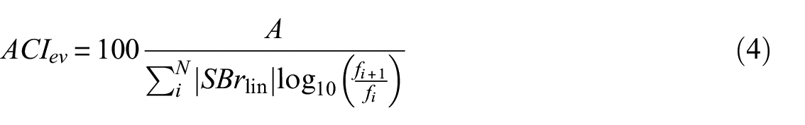
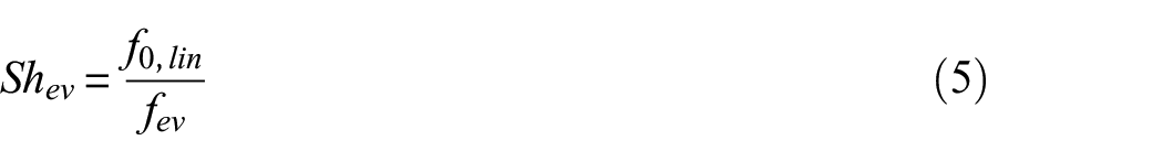
A hyperbolic tangent function can also be used to model the increase in damping and reduction of the shear modulus with increasing deformation, and it is therefore well suited for describing nonlinear soil behavior (Castro-Cruz et al., 2020; Régnier et al., 2013). The ACI_ev and Sh_ev with increasing PGA_B for the example station FKSH12 is shown in Figure 5a and b, along with the fitted hyperbolic function (blue lines). The hyperbolic function, ACI_ev and Sh_ev for a second example station IBRH14 is shown in Figure S3 in Supplement Material:

1. From the fitted hyperbolic tangent function of each station, we derive a set of parameters that are used to characterize the nonlinearity for the particular site. The hyperbolic tangent function consists of three stages; the first flat (linear) stage, then an increasing (nonlinear) stage, and finally a flattening (stabilization) stage. From this curve we extract two types of site-specific nonlinearity parameters: the station’s degree of nonlinearity, selected as the a coefficient for the hyperbolic tangent function, which represent the midpoint of the nonlinear stage between the linear and stabilization stages

2. The PGA threshold for onset of nonlinearity, selected as the PGA where the curve surpass 5%

Figure 5.

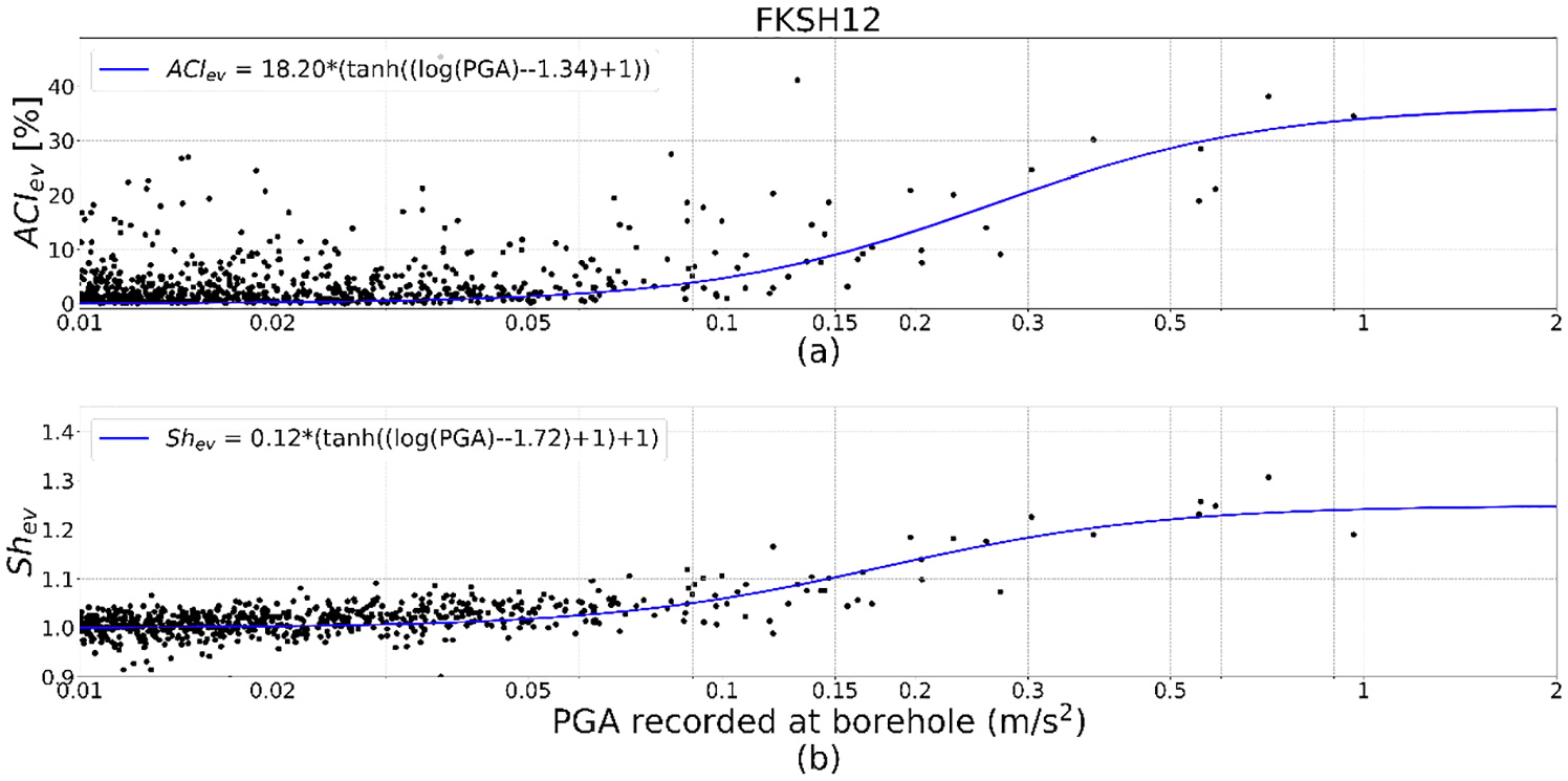
(a) The ACI_ev and (b) the Sh_ev with increasing PGA_B (black dots) and the fitted hyperbolic function (blue lines) and the uncertainty (σ) related to the curve fitting (shaded blue area).

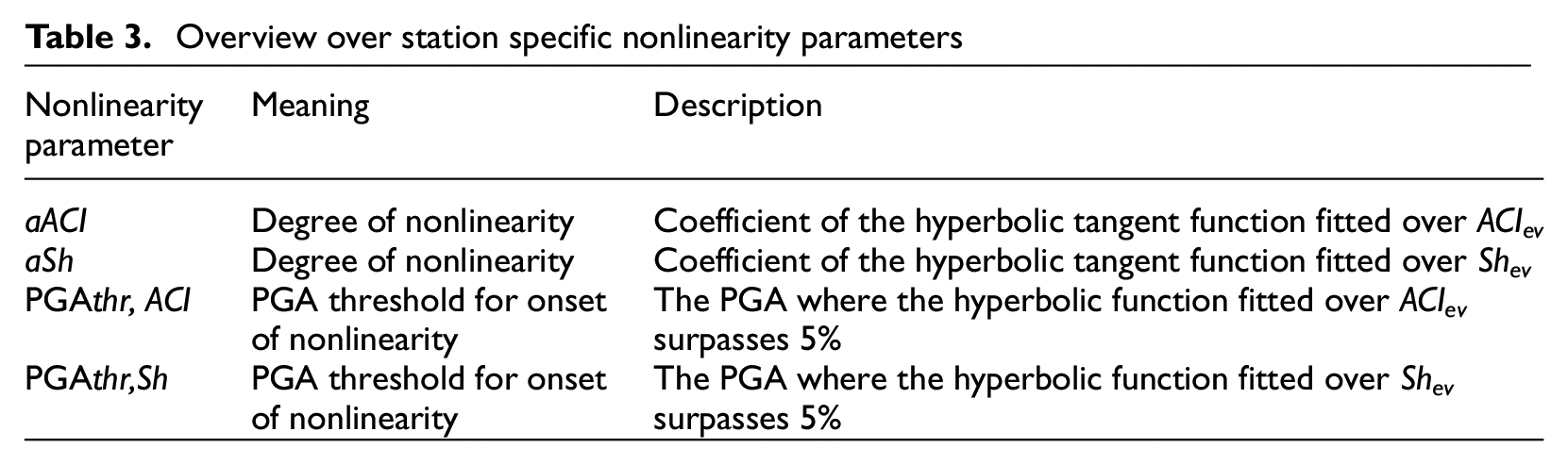
These parameters are obtained from the fitted curves for both the ACI_ev and Sh_ev measurements, resulting in four site-specific parameters, whose overview is given in Table 3. Note that this approach differs from Régnier et al. (2013), where the degree of nonlinearity is selected as the amplitude change and frequency shift predicted by the hyperbolic function at PGA = 0.05g, and only the PGA at the fitted function for amplitude change at 10% were considered.

Table 3.

Overview over station specific nonlinearity parameters

Nonlinearityparameter	Meaning	Description
aACI	Degree of nonlinearity	Coefficient of the hyperbolic tangent function fitted over ACIev
aSh	Degree of nonlinearity	Coefficient of the hyperbolic tangent function fitted over Shev
PGAthr, ACI	PGA threshold for onsetof nonlinearity	The PGA where the hyperbolic function fitted over ACIevsurpasses 5%
PGAthr,Sh	PGA threshold for onsetof nonlinearity	The PGA where the hyperbolic function fitted over Shevsurpasses 5%

Correlation between nonlinearity and site parameters

To measure the correlation between the nonlinearity parameters and the continuous site proxies, the correlation coefficient Spearman’s ρ is used. We choose the Spearman correlation, also called rank-correlation, over the more common Pearson correlation coefficient, because it does not assume a normal distribution and is less sensitive to outliers (Hollander et al., 2013; Zhu et al., 2020). The Spearman’s ρ is calculated as the Pearson correlation, but by first ranking the data within two of the variables:

$$\mathrm{Spearman}\mathrm{-}\rho =\frac{\mathrm{cov}(R\left(x\right),R\left(y\right)\}}{{\sigma }_{R\left(x\right)},{\sigma }_{R\left(y\right)}}$$

(8)

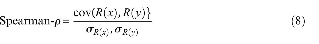
where y, R(x), R(y) are the rank vectors of the site proxy variable x and nonlinearity parameter y, and σ_R(x),σ_R(y) are the standard deviations of the rank vectors.

For the categorical site proxies, in order to capture in a single parameter, the explanatory power of a classification variable, we calculate the correlation with the pseudo–r², also used by Panzera et al. (2021) and Bergamo et al. (2022):

$$\mathrm{pseudo}-r^2=1-\frac{S{S}_{\mathrm{res}}}{S{S}_{\mathrm{tot}}}=1-\frac{{\sum }_{c=1}^n({\sum }_{k=1}^m{(x_k-{\overline{x}}_c)}^2)}{{\sum }_{i=1}^n{(x_i-\overline{x})}^2}$$

(9)

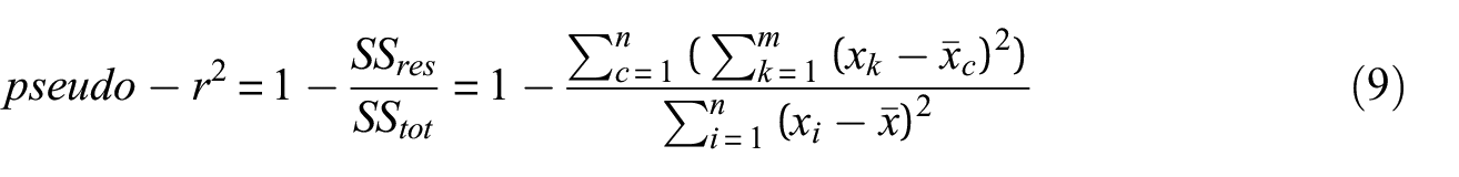
where SS_res is the sum of the squared differences between the nonlinearity parameter x_k of each site k in class c and the average of x_c for all the sites in class c, with m number of sites in a class and l number of classes. SS_tot is the total sum of squares of the difference between the nonlinearity parameter x_i of each site i and the average of the nonlinearity parameters x for all the sites, with n total number of sites. Similarly to the coefficient of determination (r²) for continuous variables, the aim of pseudo-r² is to summarize the ability of the proposed classification to sort the samples of the dependent variable into homogeneous categories. Therefore, a pseudo-r² = 1 indicates that the samples x_k are sorted in perfectly homogeneous classes (i.e. all the samples in a class have the same value); pseudo-r² = 0 indicates that the classes are not more homogeneous than the overall distribution of x variable.

Ground-motion intensities as estimators of strain level

Here, we consider four different intensity parameters as estimators of strain level; PGA_S, PGA_B, PGAemp.rock and PGVS/VS30.

PGV_S/V_S30 is generally considered as a proxy for shear strain (e.g. Brandenberg et al., 2009; Chandra et al., 2016; Gueguen et al., 2019). However, the estimation of PGV is associated with higher uncertainties related to the integration from acceleration to velocity when calculating PGV. Therefore, and because PGA is directly related to shear stress in horizontal planes, which in turn is related to strain for a given shear modulus (Seed and Idriss, 1971), PGA is often used as an alternative indicator of the level of strain induced by an earthquake on a site. When recorded at the surface, PGA_S represents the true intensity experienced at the site, but it is also affected by the nonlinearity, and therefore both a trigger and an effect of nonlinear soil behavior. PGA on rock and at depth, however, is expected to be virtually unaffected by site effects and therefore a better indicator of the strain level induced by an earthquake. However, PGA_B is also affected by the downgoing wave and does not correspond to the PGA that would be recorded at a rock outcrop at the surface.

PGA_rock recorded at surface and rock sites defined as V_S30 ≥ 760 m/s are classical ground-motion parameter and rock site conditions used on probabilistic seismic hazard maps and associated building codes (e.g. Seyhan and Stewart, 2014; Weatherill et al., 2023). To facilitate for comparisons with seismic hazard, we therefore aim to obtain a value closer to the PGA_rock recorded on the surface and propose the parameter empirical PGA on reference rock site (PGA_emp.rock), which is an approximation for the PGA recorded at a rock site (V_S30 = 760 m/s) on the surface.

To derive PGA_emp.rock, three parameters are used:

1. PGA_B: PGA recorded at the borehole.

2. PGA_S/B,lin: the mean ratio between the PGA of weak motions (PGA_S < 0.1 m/s²) recorded at surface (PGA_S,lin) and at borehole (PGA_B,lin).

3. δS2S _s : the site-term from the linear GMM derived for KiK-net from Loviknes et al. (2021). The δS2S _s used here is derived from ground motions predicted for weak motions at rock sites (V_S30 = 760 m/s), which means that δS2S _s represents the linear amplification of a site s relative to the median rock ground motion prediction (Atik and Abrahamson, 2010; Kotha et al., 2018).

PGA_emp.rock, is derived in two steps. First, PGA_B is moved to the surface using PGA_S/B,lin. In the next step, we use δS2S _s to correct the ground motion at the surface to get the motion for reference rock site conditions (V_S30 = 760 m/s).

The final empirical PGA recorded at a reference rock site at the surface then becomes:

$$\mathrm{PG}{\mathrm{A}}_{\mathrm{emp}.\mathrm{rock}}=\frac{\mathrm{PG}{\mathrm{A}}_{\mathrm{B}}\mathrm{PG}{\mathrm{A}}_{\mathrm{S}/\mathrm{B},\mathrm{lin}}}{\exp \left(\delta \mathrm{S}2{\mathrm{S}}_{\mathrm{s}}\right)}$$

(10)

Figure 6 shows PGA_S/B,lin and δS2S _s with V_S30/V_{S, B} (the ratio between V_S30 and shear-wave velocity at the borehole) and V_S30, respectively. Although the variability is high for both PGA_S/B,lin and δS2S _s , they both show a decreasing trend with increasingly stiff sites where V_S30 is high and closer to V_S,B, which is consistent with what is expected for linear site amplification and shows that the variables are reliably constrained.

Figure 6.

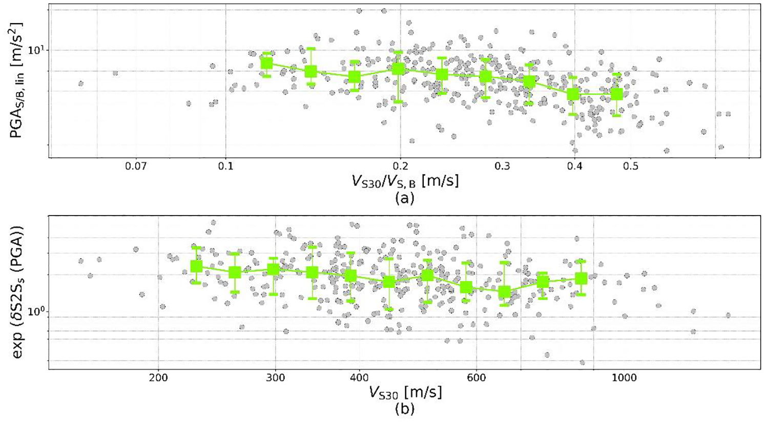
(a) PGA_S/B,lin (the mean ratio between the linear PGA recorded at surface and at borehole) as a function of the ratio between V_S30 and V_{S, B} (S-wave velocity at the borehole). (b) The site-to-site residual δS2S _s as a function of V_S30. The general trends are shown with the green error-bars representing the median and the 16% and 84% quantiles of PGA_S/B,lin and δS2S _s with V_S30/V_S,B and V_S30, respectively.

The object of deriving PGA_emp.rock is to obtain a reliable and realistic metric for PGA recorded on standard outcrop rock, in order to have a common reference for the intensity of ground motion to be able to compare the nonlinear behavior across different site conditions. An alternative to the PGA_emp.rock calculated here, is the predicted PGA on rock, adjusted for event variability using the between-event random effects (PGA_{rock, exp(}δB_e)), as done by Loviknes et al. (2021). However, to obtain the predictions on rock for all the events considered in this study a GMMs that is valid for all event types (active shallow crust, intraplate, subduction etc.) would be needed, which is challenging for such a tectonically complex region like Japan. Additional potential intensity measures for ground shaking are Cumulative amplitude velocity (CAV) and Arias Intensity, however for brevity, these will not be considered in this study.

Results

The aim of this study is not only to find site parameters that can be used to predict nonlinear site amplification but also to evaluate when (i.e. at which level of ground motion) such models should be applied. We therefore initially investigate how the amplitude change (ACI_ev) and frequency shift (Sh_ev) for all events and stations behave with increasing ground motion intensity. In the next step, we evaluate the correlation between the nonlinear soil behavior and the selected site proxies using the site-specific nonlinearity parameters derived from the curve fitting at each individual station (e.g. Figure 5).

This section summarizes first the result of the individual amplitude change (ACI_ev) and frequency shift (Sh_ev) measurements for all recorded events by all considered stations, before describing the correlation between the nonlinear site parameters and the site parameters.

Amplitude change (ACI_ev) and frequency shift (Sh_ev) for all recorded events

We compare the ACI_ev and Sh_ev for all the recorded events and stations with increasing strain using the four different intensity parameters, described above, as estimators of strain level; PGA_S, PGA_B, PGA_emp.rock, and PGV_S/V_S30 (Figures 7 and 8).

Figure 7.

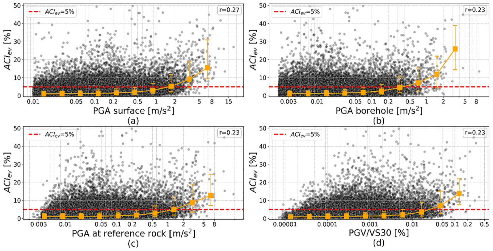
(a) The change of amplitude (ACI_ev) with increasing PGA (black dots) (a) recorded at surface, (b) recorded at borehole, (c) reference rock, and (d) PGV/V_S30. The orange squares represent the median ACI_ev with the 16% and 84% quantiles error-bars is for each intensity bin in log-scale. The correlation between each intensity parameter and the ACI_ev is given as Pearson’s correlation coefficient (r).

Figure 8.

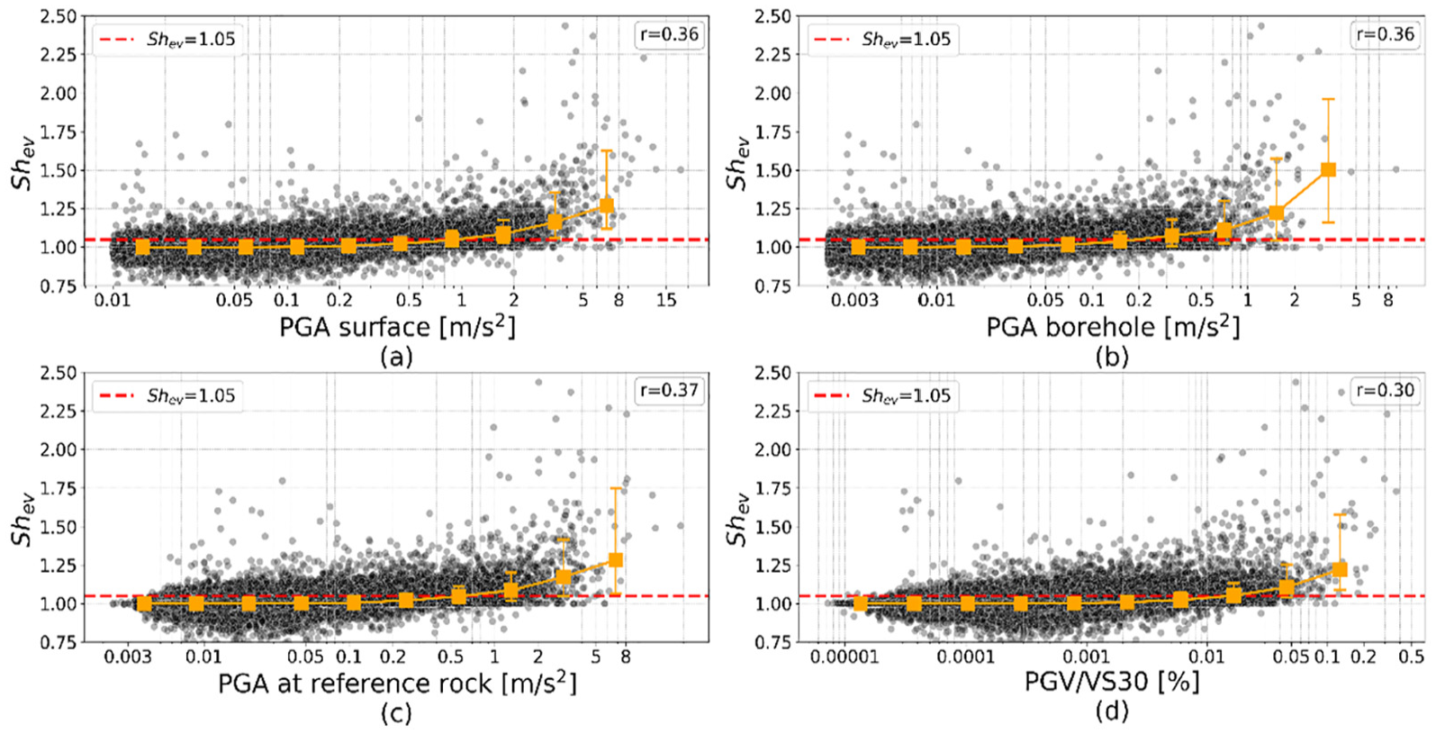
(a) The shift in frequency (Sh_ev) where Sh = 1, equals no shift and Sh > 1 are shifts toward lower frequencies, with increasing PGA (black dots) (a) recorded at surface, (b) recorded at borehole, (c) reference rock, and (d) PGV/V_S30. The orange squares represent the median Sh_ev with the 16% and 84% quantiles error-bars is for each intensity bin in log-scale. The correlation between each intensity parameter and the Sh_ev is given as Pearson’s correlation coefficient (r).

To better illustrate the general amplitude change and frequency shift, the PGA and PGV_S/V_S30 values are binned in logarithmic scale and the 16%, 50% and 84% quantiles of ACI_ev and Sh_ev are calculated for each bin (orange squares and error-bars in Figures 7 and 8), the values for each bin are given in Table S1 in Supplement Material. Figures 7 and 8 show that although there are large values and high scatter of ACI_ev and Sh_ev over the entire intensity range, the majority of the change is low and centered around 0% for low intensity but starts to increase at higher intensity. The large values at low intensity values are likely artifacts due to the threshold for recording set by KiK-net (PGA = 0.002-0.004 m/ s2, Aoi et al., 2011) as suggested by Campbell et al. (2022), or due to noisy records that cannot be detected using automatic methods. These high values at low intensities come from a few outliers, this is demonstrated by the error-bars (representing the binned median values and 16% and 84% quantiles). At high ground motion intensities, however, the high scatter is likely mainly due to few records with high-intensity values (reflected by the large quantile range) and the station-specific variability (considering that the error-bars reflect the mean values across all events and stations).

The median ACI_ev exceeds 5%, shown as red dashed lines in Figure 7, above 1.401 m/s² for PGA_S, around 0.5 m/s² for PGA_B, around 1 m/s² for PGA_emp.rock and around 0.028% for PGV/V_S30 (Table S1). The percentage of records exceeding 10% ACI is 52.26% and 68% at PGA_B = 1.2 and 2.784 m/s², respectively, which is consistent with the findings of Régnier et al. (2013). For Sh_ev the median exceeds 5% shift (Sh_ev = 1.05, red dashed line in Figure 8), at slightly lower intensity values, between 0.662 and 1.401 m/s² for PGA_S, at 0.223 m/s² for PGA_B, between 0.392 and 0.932 m/s² for

PGA_emp.rock and 0.01% and 0.028% for PGV/V_S30. The difference between ACI_ev and Sh_ev is likely due to the variability range of the linear site response, which is only considered when measuring ACI_ev, while Sh_ev is measured as the cross-correlation independent of the variance. The correlation between the intensity parameters (PGA_S, PGA_B, PGA_emp.rock and PGV_S/V_S30) and the nonlinearity measures (ACI_ev and Sh_ev) is calculated using Pearson’s correlation coefficient (r). While all the intensity parameters has a similar level of correlation (0.23–0.27 for ACI_ev, and 0.30–0.37 for Sh_ev), PGA_S has a slightly better correlation with ACI_ev and PGA_emp.rock have the best correlation with Sh_ev.

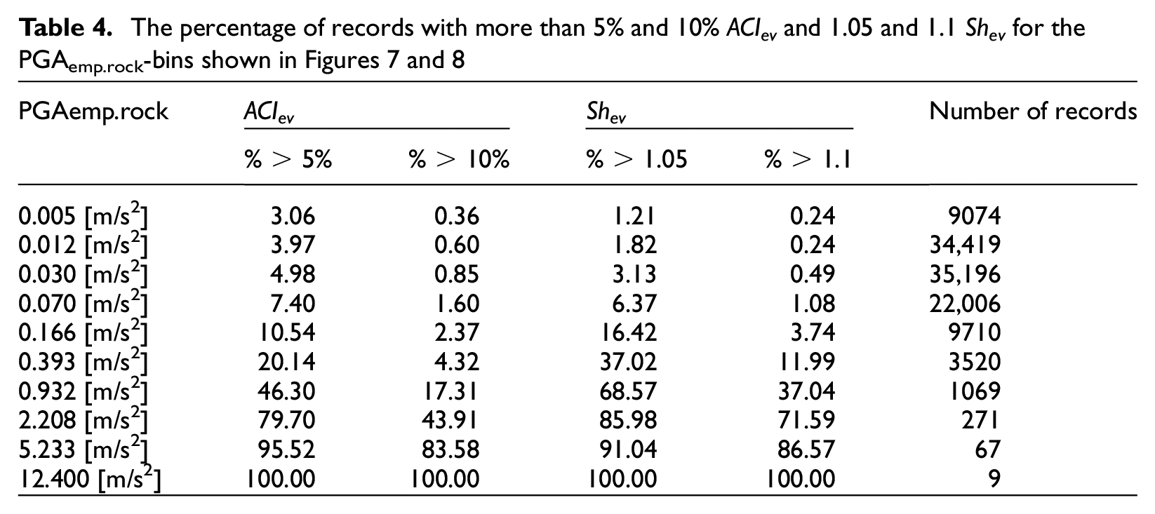
For most studies on nonlinear soil behavior at KiK-net sites, PGA recorded at borehole have been used (e.g. Castro-Cruz et al., 2020; Régnier et al., 2013, 2016), however, for comparison with ground-motions parameters used in classical probabilistic seismic hazard analysis (PSHA) models and maps, a PGA recorded at a rock surface site is needed. In the remainder of this study, we will therefore focus on the nonlinear soil behavior with PGA_emp.rock. Table 4 lists the percentage of recorded events above 5% and 10% within each PGA_emp.rock-bin in Figures 7c and 8c, along with the number of records within each bin. In a seismic hazard context, Table 4 can be used to evaluate whether nonlinear soil behavior should be taken into account for a given ground-motion intensity (PGA_emp.rock). For example, at around 1 m/s², which has been suggested as a PGA threshold for nonlinearity (Frid and Kamai, 2023; Régnier et al., 2016), only 17.31% of the 1069 records in the PGA_emp.rock-bin (with median 0.932 m/s²) have more than 10% amplitude change (ACI_ev). In the same bin, 37.04% of the records have a shift in frequency (Sh_ev) above 1.1. For stronger ground motions (e.g. PGA_emp.rock = 2.208 m/s²), the number of records per bin are still high (271), indicating that the percentage of nonlinear records are still significant, with 43.9% and 71.59% of the records exceeding 10% ACI and 1.1 shift in frequency.

Table 4.

The percentage of records with more than 5% and 10% ACI_ev and 1.05 and 1.1 Sh_ev for the PGA_emp.rock-bins shown in Figures 7 and 8

PGAemp.rock	ACIev		Shev		Number of records
	% > 5%	% > 10%	% > 1.05	% > 1.1
0.005 [m/s2]	3.06	0.36	1.21	0.24	9074
0.012 [m/s2]	3.97	0.60	1.82	0.24	34,419
0.030 [m/s2]	4.98	0.85	3.13	0.49	35,196
0.070 [m/s2]	7.40	1.60	6.37	1.08	22,006
0.166 [m/s2]	10.54	2.37	16.42	3.74	9710
0.393 [m/s2]	20.14	4.32	37.02	11.99	3520
0.932 [m/s2]	46.30	17.31	68.57	37.04	1069
2.208 [m/s2]	79.70	43.91	85.98	71.59	271
5.233 [m/s2]	95.52	83.58	91.04	86.57	67
12.400 [m/s2]	100.00	100.00	100.00	100.00	9

Parameters describing nonlinearity at each site

In the previous section, we evaluated the number of records and nonlinear behavior with increasing intensity, now we investigate how the nonlinearity correlates with site parameters. For each of the 350 KiK-net sites with V_{S, B} ≥ 760 m/s, more than one recorded strong-motion event (PGA_S ≥ 0.5 m/s²) and more than 10 linear events (PGA_S ≤ 0.1 m/s²), a hyperbolic tangent function was fitted over the measured amplitude change (ACI_ev) and frequency shift (Sh_ev) with increasing empirical PGA on reference rock. From the curve fits, a valid PGA threshold can only be obtained for the stations that have experienced sufficiently high nonlinearity for the fitted curves to surpass ACI_ev > 5% and Sh_ev > 1.05. The number of strong-motion records per station ranges between 2 and 160, with an average of 12 strong motion events recorded per station (Figure 1). Out of the 350 stations considered, we only keep the curve fits where the uncertainty related to the curve fitting coefficients is low (a_σ < 5% and b_σ < 0.5) and a valid PGA threshold were obtained, yielding 169 and 230 sets of site parameters for ACI_ev and Sh_ev, respectively.

The distribution of the site-specific parameters a_ACI, a_Sh, PGA_thr,ACI and PGA_thr,Sh derived from the fitted curves (as described in Table 3) are shown in Figure 9 and provided in Supplementary material (Supplement 2). For comparison, (Régnier et al., 2013) analyzed the 54 KiK-net sites that had recorded at least two events with PGA_borehole > 0.5 m/s² by March 2011, out of which PGA_thr,ACI were obtained for 34.

Figure 9.

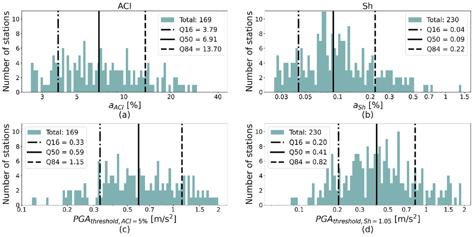
The site-specific parameters characterizing (a) degree of nonlinearity based on amplitude change (a_ACI), (b) degree of nonlinearity based on frequency shift (a_Sh), (c) PGA threshold for onset of nonlinearity, defined as the PGA where the amplitude change exceeds 5% (PGA_thr,ACI) and (d) PGA threshold for onset of nonlinearity, defined as the PGA where the shift in frequency exceeds 1.05 (PGA_thr,Sh).

The distribution of site-specific parameters in Figure 9 shows that most stations have a low degree of nonlinearity, with 84% of the stations having a degree nonlinearity based on change in amplitude a_ACI < 13.7% (Figure 9a) and based on frequency shift a_Sh < 0.22 (Figure 9b). The PGA thresholds also have a wide variance, with most stations (68%) having a PGA threshold between 0.33 and 1.15 m/s² for ACI (Figure 9c) and between 0.2 and 0.82 m/s² for Sh (Figure 9d). Moreover, both the degrees of nonlinearity (a_ACI and a_Sh) and the PGA thresholds (PGA_{thr, ACI} and PGA_thr,Sh) appear to have a lognormal distribution, we, therefore, consider the nonlinearity site parameters on a logarithmic scale for the correlation with the site proxies in the remainder of this study.

Correlation between nonlinearity and geotechnical and site-specific (direct) site parameters

We first examine the correlation between the nonlinear site parameters and the direct site proxies A_p, f₀, V_S30, and Z_S0.8 (Figure 10). To demonstrate the general trend of the nonlinearity parameters with the site proxies, the 0.16, 0.5, and 0.84 quantiles of the nonlinearity parameters are computed for the direct site proxies (blue error-bars) using bins defined as fractions of interquartile range.

Figure 10.

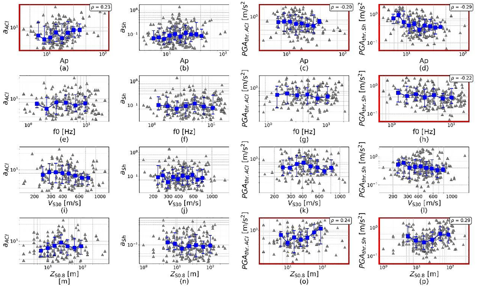
The site-specific nonlinearity parameters a_ACI (left) a_Sh (middle left), PGA_{thr, ACI} (middle right), and PGA_thr,Sh (right) against the direct site proxies A_p (top row, a to d), f₀ (second top row, e to h), V_S30 (second bottom row, i to l), and Z_S0.8 (bottom row, m to p). The Spearman correlation coefficients ρ for the significant correlation pairs (p-value < 0.05) are given in the plots, these pairs are also marked with red thick frames around the subplot.

The degree of correlation between each nonlinearity parameter and site proxy pair is summarized by the Spearman correlation coefficient ρ. Only the correlations with p-value < 0.05 are considered significant, these pairs are marked with red thick frames around the subplot (Figure 10a, c, d, h, o, and p) and summarized in the heatmap in Figure 11a.

Figure 11.

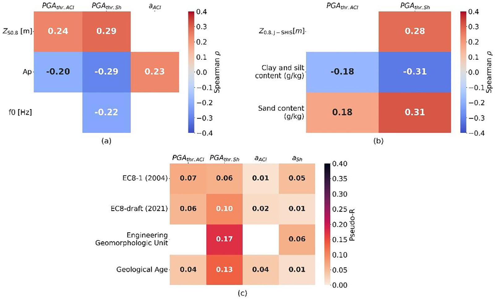
The correlation coefficient between the site-specific nonlinearity parameters and the (a) direct site parameters, (b) indirect site proxies, and (c) categorical site proxies. Note that the correlation coefficients are shown only when the relation between the nonlinearity parameter and the site proxies is significant. For the Spearman correlation coefficient ρ the correlation is significant if the associated p-value is < 0.05 and the pseudo−r² is considered significant if the percentage of classes with more than 10 stations is greater than 50% of all available categories. The non-significant relations are either shown as white squares or excluded from the heatmaps.

Figures 10 show that the nonlinearity parameters have a large variability from one station to another, particularly the degrees of nonlinearity, a_ACI and a_Sh, which also generally have a low correlation with the site proxies (ρ < 0.3) and high p-value (>0.05). Only the maximum amplitude of the linear site response (A_p) has a significant correlation with a_ACI (ρ = 0.23, Figure 10a), with higher A_p, meaning that sites with high linear site amplification have a higher degree of nonlinearity.

For the PGA threshold based on the shift (PGA_thr,Sh), there is as significant inverse correlation with A_p (ρ = −0.29), the fundamental resonance frequency f₀ (ρ = −0.22) and depth to V_S = 800 m/s (ρ = −0.29). A_p and Z_S0.8 also have the highest correlation and a significant correlation with PGA_{thr, ACI}. The correlation between A_p and the PGA thresholds shows that sites with higher amplitudes start to show nonlinear soil behavior at lower PGAs but may also indicate that the nonlinearity parameters contain both the linear and nonlinear site amplification. The higher correlation between Z_S0.8 and both the PGA thresholds suggests that depth to bedrock is the most promising of the direct site parameters and shows that shallow sediments have an earlier onset for nonlinearity (Figure 10 o and p).

Notably, the classical site proxy V_S30, shows no significant correlation with the nonlinearity site parameters. As previously discussed, several studies have already suggested that V_S30 is not a suitable proxy for nonlinearity as sites with similar values can exhibit different susceptibility to nonlinear response (e.g. Bonilla et al., 2011; Régnier et al., 2013). However, considering that V_S30 is still a much-used proxy for nonlinear site response, this result is still relevant. Due to the borehole-configuration of the KiK-net sites, several other VS-parameters are available for these sites (Zhu et al., 2020). Additional correlation between the nonlinearity parameters and a selection of these VS-parameters have been explored, however, a significant correlation was not obtained for any of the VS-parameters, this is demonstrated in Figure S4 in Supplement Material.

Correlation between nonlinearity and indirect site proxies

As with the direct site proxies, the correlation between the nonlinearity parameters and the indirect site proxies is evaluated using the Spearman correlation coefficient ρ. Interestingly, the correlation between the nonlinearity parameters and the indirect site proxies is similar to the correlation with most of the direct proxies, which is generally not the case, at least when dealing with linear site response (Bergamo et al., 2022). However, as with the direct site proxies, the correlation between the nonlinearity parameters and the indirect site proxies is low. This is demonstrated by the absolute Spearman correlation coefficient |ρ| ranging from 0.18 to 0.31 for the PGA thresholds (Figures 11b, 12d, g, h, k and l). The indirect proxies with the highest correlation with the nonlinearity parameter are for depth to V_S = 800 m/s from the J-SHIS velocity map (ρ = 0.28, Figure 12d) and the globally available values from SoilGrid (|ρ| = 0.31, Figure 12h and l). For all these values, the highest correlation is with PGA_thr,Sh, however, the SoilGrid values also have a significant, though lower, correlation with the PGA threshold based on amplitude change (|ρ| = 0.18). When comparing soils with a higher fraction of sand to soils with higher fractions of clay, laboratory tests prescribe an onset of nonlinearity at lower strain levels for soils with a higher fraction of sand (e.g. Ciancimino et al., 2020). Notably, the trends between the PGA thresholds and clay and silt (Figure 12g and h), and sand (Figure 12k and l), observed here, are the opposite of what is observed in laboratory tests. However, at the measurement scale of seismic stations, finer and softer sediments like clay produce higher amplification than coarser materials like sand, hence higher strain levels and an earlier onset of nonlinearity (earlier = lower levels of PGA on rock).

Figure 12.

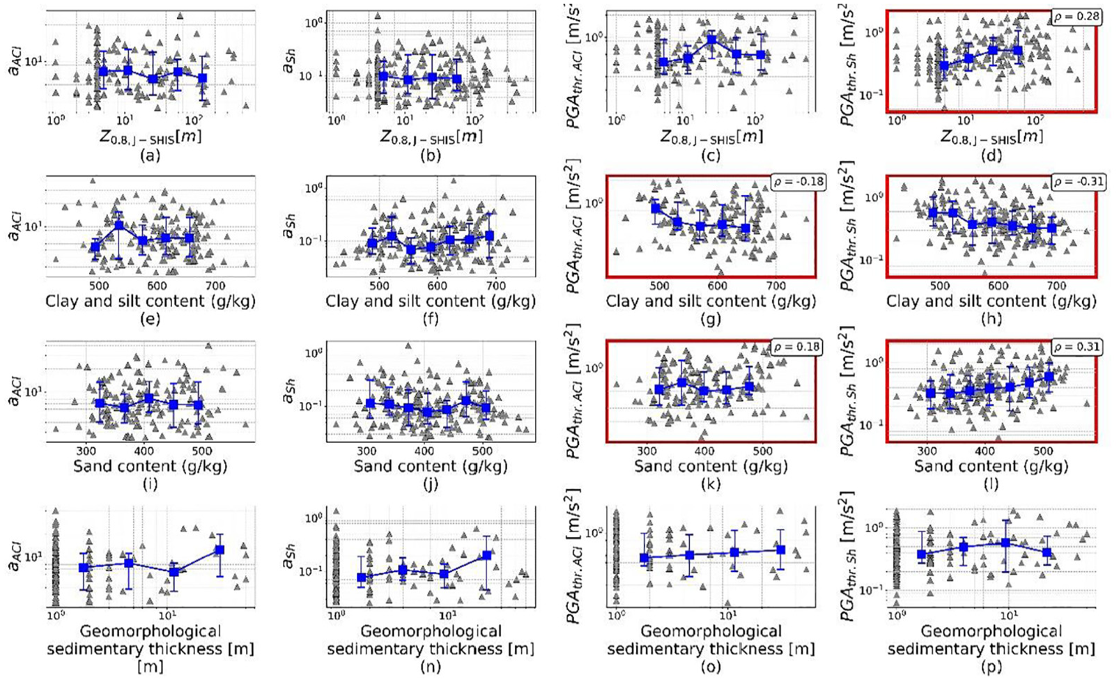
The site-specific nonlinearity parameters a_ACI (left) a_Sh (middle left), PGA_{thr, ACI} (middle right) and PGA_thr,Sh (right) against depth to S-wave velocity 0.8 km/s Z_0.8 derived from J-SHIS (top row, a-d), Clay content (second row, e-h) and Sand content (second to bottom row, i-l) derived from SoilGrid, and Geomorphological sedimentary thickness from Pelletier et al. (2016) (bottom row, m-p). The Spearman correlation coefficients ρ for the significant correlation pairs (p-value < 0.05) are given in the plots, these pairs are also marked with red thick frames around the subplot.

Correlation between nonlinearity and categorical site proxies

Finding a relation and calculating the correlation with categorical site proxies is more challenging to both demonstrate and quantify, than with continuous site parameters, as the categorical proxies represent a categorization of the sites into discrete values rather than a continuous relation (Bergamo et al., 2022). The pseudo–r² correlation is calculated for all of the nonlinearity parameter-categorical site proxy pairs but is only considered reliable for those pairs where the percentage of site proxy classes with more than 10 stations is above 50% (Figure 11c). Figure 11c shows that the correlation between the nonlinearity and the categorical site proxies is weak with the highest correlation reaching pseudo–r² = 0.17 between the PGA threshold based on the shift (PGA_thr,Sh) and the Engineering Geomorphologic Unit from Wakamatsu and Matsuoka (2013) and pseudo–r² = 0.13 with the geological ages from (Geological Survey of Japan, 2015, SDGM).

This weak correlation may be due to the uneven distribution of stations within each categorical site group (Figure 3e to h) and the high variability of the nonlinearity parameters (Figure 9) also within the categorical groups, as shown in the boxplots for the PGA threshold based on the shift with the categorical site proxies (Figure 13). The boxplots for the degree of nonlinearity and the PGA threshold based on amplitude change are shown in Figures S5, S6 and S7, respectively, in the Supplement Material. In addition, the distribution of the fundamental frequency (f₀) within each categorical site group is shown in Figure S5.

Figure 13.

Boxplots showing the distribution of the PGA threshold based on the shift (PGA_thr,Sh) with the categorical site proxies (a) Eurocode 8 (EC8-1) soil classes based on V_S30, (b) new Eurocode 8 soil classes (EC8-draft) based on Z_S0.8 and V_{S, H}, (c) geological age and (d) Engineering Geomorphological Unit.

Figure 13 shows that for both the EC8-1 and EC8-draft soil classes, the classes A and B have a median close to the median of the whole data set, while the medium stiff class C has a higher median (i.e. a “later” onset of manifest nonlinear behavior). The lower median PGA threshold for the stiff soil classes A and B, compared to C, could be caused by shallow layers of softer sediments, which is also indicated by the high median fundamental frequency for these classes (Figure S8a and b). The median PGA threshold for soft soil class D, however, is slightly below the median of the whole data set only with the EC8-1 classification, while with the new EC8-draft classification, class D has a higher median PGA threshold. This is probably due to the change in the V_S30 range for the new EC8-draft classification, where soft soil is defined as 150 m/s ≤ V_{S, H} < 250 m/s, while in for EC8-1, D is defined as using V_S30 < 180 m/s (Tables 1 and 2).

For class E, representing soft thin sedimentary layers, the median PGA threshold for both the EC8-1 and EC8-draft classifications is lower than for the other classes, indicating that such sites have an earlier onset of nonlinearity. This is consistent with the findings from the correlation between the PGA thresholds and parameters for depths to bedrock and sediment thickness (Z_0.8, Z_{0.8, J−SHIS} and Geomorphological sedimentary thickness) where lower PGA thresholds are found for thin sediment layers and shallow depths to bedrock.

For geological age, Late Pleistocene to Holocene and Tertiary have the same distribution as the whole data set, while Holocene, Late, Middle, and Early Pleistocene all have a higher median PGA threshold and Pre-Tertiary has a lower median PGA threshold than the other geological ages (Figure 13c). Notably, for the Quaternary sediments (Holocene, Late, Middle, and Early Pleistocene), the PGA threshold appears to increase with age of deposition, which is likely related to the fact that recent material is less compacted, not cemented, and thus more prone to earlier onset of nonlinearity. For Pre-Tertiary, the lower threshold may be caused by thin layer of Quaternary sediments overlying shallow Pre-Tertiary bedrock, which is also indicated by Pre-Tertiary’s high median fundamental frequency in Figure S5c in Supplementary material.

When using the Engineering Geomorphologic Unit classification of (Wakamatsu and Matsuoka, 2013), the PGA threshold distributions of each unit (Figure 13d) have a wider distribution than the Eurocode classes and the geological age, which is also demonstrated by the higher pseudo–r². Some of the units with a higher number of stations, Hill, Volcanic Footslope and Valley bottom lowland, have medians close to those of the whole data set and thus do not add new information. Still, the Mountain unit, which has the highest number of stations, has a clear lower PGA threshold median, which may indicate that this unit consists of thin sediment layers (also indicated by the high median fundamental frequency in Figure S8d in Supplementary material) causing earlier onset of nonlinearity. The Gravelly Terrace and Alluvial Fan units, which consist mainly of gravel and course material where severe nonlinearity is not expected, as well as the typically stiff Mountain Footslope and Terrace covered with volcanic ash soil units, have higher PGA threshold distributions centered above the median of the entire data set. Conversely, the Deltas and Coastal Lowlands units are composed of finer material, which amplifies more and has an earlier onset of nonlinearity, as indicated by the low PGA threshold distribution.

Discussion

Limitations on the measurements of nonlinearity and the estimation of the nonlinear site parameters

While the result showed some correlation between the site-specific PGA thresholds and the site proxies, especially for the PGA threshold based on shift in frequency (PGA_thr,Sh), the correlation between the degree of nonlinearity a and the site proxies were mostly low or none at all, suggesting that the a parameter is not a robust nonlinearity parameter. One possible explanation is that the a coefficient for the hyperbolic tangent function represents the midpoint of the nonlinear stage between the linear and the stabilization stage. If a station has not experienced its full possible range of shaking intensities, the a coefficient will depend on a few data points and therefore will not be robustly estimated and may not be representative of the stabilization stage.

The PGA thresholds, however, represent the PGA at which the nonlinearity curves exceed a given threshold (here 5%) and can therefore be considered as more independent of whether a station actually recorded its full PGA-range, as long as the curves actually exceed the threshold. A limitation of the PGA thresholds is therefore that for stations with low levels of nonlinearity, even for high-intensity events, the PGA threshold is not obtained and therefore excluded from our successive analyses. This possibly results in a disproportionately low number of stations with high PGA thresholds and could potentially bias the correlation with the site proxies. An alternative solution would be to set all non-valid PGA thresholds to a high number, but this could introduce a different type of bias.

When comparing the two PGA thresholds, the PGA threshold based on shift in frequency (PGA_thr,Sh) has a significant relationship with the most site proxies and the highest correlation for all site proxies. The difference between the two PGA thresholds is likely to be mainly due to a valid PGA_{thr, ACI} being obtained for fewer stations than PGA_thr,Sh (Figure 9). An additional cause could be that the shift in frequency measurements (Sh_ev) is better constrained than ACI_ev. This is also suggested by the high scatter of amplitude change measurements (ACI_ev) over the entire PGA-range as shown in Figure 7, compared to Sh_ev (Figure 8). This is likely due to the amplitude change induced by nonlinear site effects being caused by two effects; both the damping (reduction in amplitude) at high frequencies and the shift in frequency caused by the reduction in shear modulus at low frequencies. In comparison, the shift in frequency is only caused by the shear modulus reduction. To overcome this issue, and potentially make the amplitude change measurements more stable, the change in amplitude should therefore be measured separately before and after the fundamental frequency, but this would require a longer frequency range than used here (<21 Hz) and more certainty on the selection of the fundamental frequency. Alternatively, the amplitude change could be measured for each frequency independently instead of spanning the whole frequency band, thus yielding a frequency-dependent amplitude change vector. Such a frequency-dependent nonlinearity parameter could also potentially improve the correlation with the site proxies considering that most site proxies only correlate well with site response in certain frequency ranges, for example, topography for low frequencies and V_S30 for intermediate frequencies (Bergamo et al., 2022). However, this approach is outside the scope of the current study.

In addition, the ACI_ev measurements also depend on the variability of the linear site response, which can introduce additional uncertainty. Unlike Sh_ev, which is measured using cross-correlation between each event and the mean linear site response, ACI_ev is measured as the area outside the 5% and 95% quantiles of the linear site response. Because several effects can have an impact on the variability of the linear site response, including 2-D or 3-D effects (Pilz and Cotton, 2019; Zhu et al., 2022) and temporal variations (Bonilla and Ben-Zion, 2020), the choice of variability range around the linear site response can affect the measurements of the amplitude change associated with nonlinear soil behavior. In future studies, investigations of such effects should therefore be performed, but this is beyond the scope of this study.

KiK-net sites are widely used for site response analysis due to the large number of weak and strong ground motion records, and the readily available rock reference from the borehole record. However, it has been suggested that the nonlinear soil behavior observed for KiK-net sites is less prominent than for other networks and regions (e.g. Campbell et al., 2022; Gueguen et al., 2019). And although other networks with similar borehole configurations certainly exists, for example, in California (Garner Valley downhole array, Archuleta et al., 1992), Taiwan (e.g. Beresnev et al., 1995; Kuo et al., 2018) and Greece (ARGONET, Theodoulidis et al., 2018). These are not as large-scale, have not recorded as many strong motions, and/or are not as easily accessible as KiK-net. Alternatively, for sites without borehole instruments, the nonlinearity could be measured using HVSR instead of SBr (e.g. Régnier et al., 2013; Ren et al., 2017; Wang et al., 2023; Zhou et al., 2020) but, as demonstrated by Régnier et al. (2013), the amplitude change is not as accurately estimated when using only HVSR.

Furthermore, in a study exploring nonlinear site response in Lucerne, Switzerland, the site-specific hyperbolic functions in this study were compared to numerical simulations of nonlinear site amplification (Janusz et al., 2024). Although there was a high discrepancy between the hyperbolic functions and the simulations allowing for liquefaction (with excess pore water pressure), this is likely due to the paucity of empirical observations of liquefaction recorded by the KiK-net stations and the relatively deep-water table in Japan in comparison to the site tested in Switzerland. For simulations that did not allow for excess pore water pressure (without strong pore pressure and not allowing for liquefaction) the empirical hyperbolic functions from KiK-net exhibited a high degree of correlation with the simulated nonlinear behavior for Switzerland (Janusz et al., 2024). This result indicates that there is a consistency between the estimated and observed nonlinearity across regions. Another limitation with KiK-net sites, is that they are situated on predominantly stiff site conditions due to their borehole configuration and are on average harder than K-NET sites (Aoi et al., 2004, 2011). However, according to the V_S30 distribution of the sites considered in this study (Figure 2d) a wide range of soil types (in terms of V_S30) are represented. For these reasons, therefore, we argue that the nonlinearity measurements from KiK-net are valid, while at the same time acknowledging the need for expanding such systematic analysis of nonlinearity to other strong motion networks beside KiK-net.

Implications of the results

The low correlation (|ρ| ≤ 0.31) and high variability (Figures 10 and 12) between the nonlinearity site parameters and the site proxies suggest that nonlinear soil behavior is too site-specific to be captured by a single proxy. Therefore, future studies should investigate the ability of multiple indirect site proxies in combination to predict nonlinear soil behavior.

Out of the geotechnical and site-specific site parameters, depth to bedrock (Z_S0.8) and fundamental frequency (f₀) have the highest correlation with the PGA threshold (|ρ| ≥ 0.22), with earlier onset of nonlinearity (low PGA threshold) for shallow depths and high f₀, indicating that sites with thin sediment layers over rock are particularly prone to an earlier onset of nonlinear soil behavior. A similar result is found for the indirect proxies, where the PGA threshold has the highest correlation (|ρ| ≥ 0.28) with depth to bedrock derived from J-SHIS (Z_{0.8, J−SHIS}) and the SoilGrid parameters; clay and silt, and sand content. The SoilGrid parameters are particularly promising as they are available globally. Future studies could therefore explore the possibility of combining SoilGrid parameters with other proxies to predict nonlinear soil behavior on a regional scale, also outside of Japan, or on a global scale.

Although the categorical proxies generally have a low correlation with the site parameters for nonlinearity (pseudo–r² ≤ 0.17), considering the result of the correlation with the continuous site proxies with Z_S0.8 having the highest correlation, we would argue that the new EC8-draft soil classification which is based on Z_S0.8 has the most potential among the explored categorical proxies. To further investigate the nonlinear soil behavior within each site group, we group the amplitude change and frequency shift of each event and station with the EC8-draft soil classes. The percentage of records with amplitude change (ACI_ev) more than 10% and frequency shift (Sh_ev) > 1.1, is then calculated for 10 equally spaced (in log-scale) PGA_emp.rock-bins, as shown in Figure S9 in the Supplementary material. Only the PGA_emp.rock-bins with at least 10 records per bin were considered, the number of records per bin is given in Figure S10 in the Supplementary material. The percentage of recorded events with significant nonlinearity, defined here as ACI_ev > 10% and Sh_ev > 1.1, with increasing PGA_emp.rock is shown in Figure 14. Note that this definition of significant nonlinearity is different from the PGA threshold for the onset of nonlinearity obtained for each station, which is defined as the PGA where the amplitude change, and frequency shift exceed 5% (ACI_ev > 5% and Sh_ev > 1.05).

Figure 14.

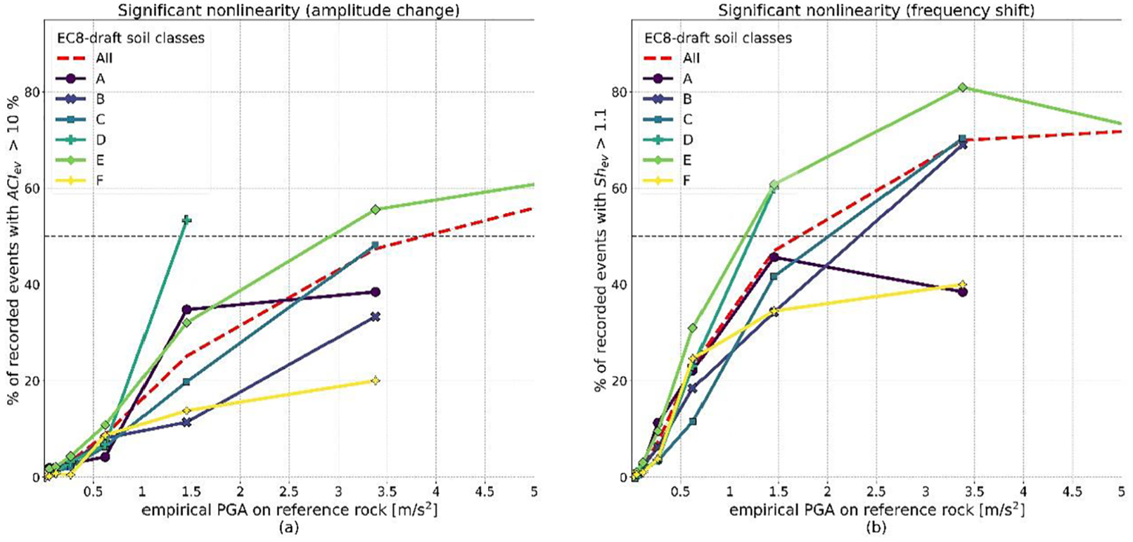
The percentage of recorded events with significant nonlinearity for (a) amplitude change (ACI) and (b) shift in frequency (Sh) within each EC8-draft soil class (Paolucci et al., 2021) with increasing PGA_emp.rock (VS30 =760m/s). Significant nonlinearity is here defined as ACIev>10% for amplitude change and Sh_ev > 1.1 for shift in frequency.

In seismic hazard and risk assessment, dealing with nonlinear site effects does not only concern how to model but also when to take the nonlinear site amplification models into account. We believe our study, with its wealth of record-by-record and site-specific measurements of nonlinearity, particularly contributes to tackle the latter issue, that is, at which level of ground motion or hazard (captured by PGA_emp.rock) nonlinear soil behavior starts to significantly affect site response (Table 4 and Figure 14). In addition, the results of our study might serve as empirical comparison for numerical simulations of nonlinear soil response (e.g. Janusz et al., 2022). Furthermore, we provide insights on which site conditions are more prone to show an earlier onset of nonlinearity. When testing nonlinear site amplification models against empirical data, Loviknes et al. (2021) showed that classical nonlinear models may overpredict the deamplification due to nonlinear behavior for moderate intensity shaking up to 0.2g (≈2 m/s²), and the application of such models to moderate seismic risk countries is questionable. Figure 14, shows that although most records have a significant frequency shift (Sh_ev > 1.1) in the PGA_emp.rock-range 1–2.5 m/s² the amplitude of the site response, which is what site amplification models primarily focus on, is significant (ACI_ev > 10%) for the majority (50%) of the ground motions below 2 m/s² only for soft soil sites with intermediate sediment depth (class D). Above PGA_emp.rock = 3 m/s², only site class E (soft soil sites with thin sediment layer) exceed more than 50% of the records with significant nonlinearity (ACI > 10%). The other site classes do not contain more than 10 stations per PGA_emp.rock-bin above 3.2 m/s² where the site classes B and C (stiff and medium stiff sites) only reaches a maximum of 48% and 30% of the records showing significant nonlinearity. Considering both amplitude change and frequency shift, the percentage of significant nonlinear records for the stiff sites with thin sediment layers (A) and soft sites with deep sediment layers (F), flattens out between 1 and 2 m/s² and does not reach 50%. When combining all sites (shown by the dashed red lines in Figure 14) the percentage of significant amplitude change (ACI_ev > 10%) exceeds 50% around PGA_emp.rock = 4 m/s².

Conclusion

In this study, we have systematically quantified nonlinear soil behavior for increasing ground-motion intensity recorded by 350 KiK-net stations and derived site-specific parameters characterizing the degree of nonlinearity and the PGA threshold for onset of nonlinear soil behavior for 169 and 230 sites, in terms of amplitude change and shift in frequency, respectively. Our results show that the site-specific nonlinearity is highly variable from one site to another and that for the majority of sites (68%) the PGA threshold for frequency shift and amplitude change combined ranges between 0.2 and 1.15 m/s². When investigating the relation between the nonlinear site parameters and geotechnical and geological site parameters, parameters for depth to bedrock and characterization of the shallowest part of the soil layer display potential for predicting nonlinear site amplification. However, for all site parameters, the correlation is generally low, suggesting that a single site parameter is not sufficient to capture the nonlinear soil behavior. As proxy for the level of ground motion, we propose the parameter empirical PGA on reference rock site (PGA_emp.rock), obtained, for each considered record, as an empirical estimate for the PGA that would be recorded at a standard outcropping rock site (V_S30 = 760 m/s). For empirical PGA on reference rock above 3 m/s², we find that the majority (more than 50%) of all recorded ground motion have significant nonlinear site amplification, here defined as an amplitude change above 10%. While in the range 1 < PGA_emp.rock < 3 m/s², nonlinear soil behavior is only significant for soft soil stations with thin or intermediate sediment thickness. These results indicate for the PGA-range 1–3 m/s², nonlinear soil behavior should be considered in seismic hazard assessment only for soft soil sites with either intermediate or thin sediment thickness. However, considering that the majority of all sites combined have a significant frequency change (Sh_ev > 1.1) from around PGA_emp.rock > 2 m/s², and that most site classes do not contain more than 10 stations per PGA_emp.rock-bin above 3.2 m/s², we would argue that for PGA_emp.rock > 3 m/s² nonlinearity should be considered significant for all soil types. In conclusion, this study demonstrates that for empirical PGA on reference rock above 3 m/s² nonlinear soil behavior is highly site-specific and that finding site parameters capable of predicting nonlinear site amplification remains a challenge. These findings are constrained to the employed network (KiK-net), in future studies, therefore the analysis should be expanded to additional networks and regions.

Research data and code availability

The ground motion data were downloaded from https://www.kyoshin.bosai.go.jp/ (last accessed 7 January 2024), an updated version of the ground-motion flatfile is available at https://doi.org/10.5880/GFZ.LKUT.2025.001 (Loviknes et al. 2025). The site database of Zhu et al. (2021) was downloaded from https://figshare.com/s/e9560cb5b3516a596f78 (last accessed 12 May 2021). The SoilGrid values were downloaded from https://soilgrids.org/ (last accessed 20 March 2022) and the Pelletier et al. (2016) geomorphological sediment thickness was downloaded from https://doi.org/10.3334/ORNLDAAC/1304 (last accessed 26 January 2021). The code for computing the amplitude change (ACI), frequency shift (Sh) and the site-specific nonlinearity parameters is available at Zenodo: https://zenodo.org/doi/10.5281/zenodo.11104872

Supplemental Material

sj-pdf-1-eqs-10.1177_87552930251325729 – Supplemental material for Systematic assessment of nonlinear soil behavior at KiK-net sites in Japan: Thresholds and controlling site factors

Supplemental material, sj-pdf-1-eqs-10.1177_87552930251325729 for Systematic assessment of nonlinear soil behavior at KiK-net sites in Japan: Thresholds and controlling site factors by Karina Loviknes, Paolo Bergamo, Donat Fäh and Fabrice Cotton in Earthquake Spectra