Empirical ground-motion basin response in the California Great Valley,Reno,Nevada,and Portland,Oregon

Abstract

We assess how well the Next-Generation Attenuation-West 2 (NGA-West2) ground-motion models (GMMs), which are used in the US Geological Survey’s (USGS) National Seismic Hazard Model (NSHM) for crustal faults in the western United States, predict the observed basin response in the Great Valley of California, the Reno basin in Nevada, and Portland and Tualatin basins in Oregon. These GMMs rely on site parameters such as the time-averaged shear-wave velocity (V_S) in the upper 30 m of Earth’s crust (V_S30) and depths to 1.0 and 2.5 km/s shear-wave isosurfaces (Z_1.0 and Z_2.5) to capture basin effects and were developed using observations and simulations primarily from the Los Angeles region in southern California. Using ground-motion records from mostly small-to-moderate earthquakes and mixed-effects regression analysis, we find that the GMMs perform well with our local basin-depth models for the California Great Valley. With our local basin-depth models for Reno, the GMMs do not perform as well for this relatively shallow basin and exhibit little sensitivity to the basin parameters used in the NGA-West2 GMMs. We also find good performance for the local Z_1.0 model across the Portland region, whereas the local Z_2.5 model provides little predictive power except at sites in the deepest part of the Tualatin basin. Additional work could improve the performance of the site and basin terms in the NGA-West2 GMMs for regions with geologic structure different than the deep basins in southern California and the Great Valley. In addition, we find significant discrepancies among the GMMs in how the uncertainty in the ground motion varies with basin depth and pseudospectral period. Our results can help guide seismic hazard analyses on whether to include these local basin-depth models.

Introduction

The US Geological Survey’s (USGS) National Seismic Hazard Model (NSHM) (Petersen et al., 2023) uses empirical ground-motion models (GMMs) to estimate the earthquake shaking hazard across the United States. The GMMs require various parameters related to the earthquake source, wave propagation path, and local site conditions as inputs. Modeling of ground motions related to the local site can be further refined by accounting for effects of shallow and deep sediments, two-dimensional (2D) and three-dimensional (3D) basin geometry, and topographic focusing. Basin response is a complex physical phenomenon that combines the effects of amplification of long-period seismic waves and attenuation of high-frequency energy due to deep sedimentary sequences, and effects of 3D geometry of geologic basins, including conversion of body waves to surface waves, reflection, refraction, focusing of waves trapped within the basin structure, attenuation of seismic waves at shorter periods, and basin-edge effects (e.g., Frankel and Vidale, 1992; Graves et al., 1998; Pitarka et al., 1998).

The 2018 update of the USGS NSHM included for the first time specific regions where the effects of deep sedimentary basins (where the depth of the 1.0 km/s shear-wave isosurface, Z_1.0, is greater than 0.5 km) were considered (Powers et al., 2021). These regions encompass the greater Los Angeles area and the San Francisco Bay region in California; the Puget Lowlands, including Seattle, in Washington State; and the Wasatch Front, including Salt Lake City, in Utah. Moschetti et al. (2018) described a framework for incorporating regional- and urban-scale seismic hazard studies into the NSHM, and our work to expand the geographic footprint of the regions given special treatment for basin effects follows the spirit of that editorial.

The 2023 update of the USGS NSHM seeks to include a few additional regions with local sedimentary basin models with future updates potentially including such models over larger regions. In this study, we assess whether including local basin models for the Great Valley in California, the Reno and Sparks region in Nevada, and the Portland and Tualatin region in Oregon improves empirical ground-motion predictions. The Great Valley is one of the largest geologic features in California, and including it as a local basin within the NSHM would substantially expand the fraction of the state covered by local basin models. Past studies in both the Reno and Portland regions have found ground-motion amplification associated with sedimentary basins (Eckert et al., 2021; Frankel and Grant, 2020). Other recent studies of basin amplification focused on the comparisons of simulated and recorded ground-motion data sets in western US basin environments (e.g., Thompson et al., 2020 in Seattle; Moschetti et al., 2024, in southern California), non-ergodic, spatially varying site response models (Parker and Baltay, 2022 in southern California; Sung and Abrahamson, 2022 in the Puget Sound), or using GMMs that predict Fourier amplitude spectra (Moschetti et al., 2021; Rekoske et al., 2021). Although Fourier amplitude spectra are simpler to interpret and less dependent on magnitude, our analysis focuses on response spectral intensity measures (IMs) given that these are the primary parameters for GMMs currently used in the NSHM (refer to Rezaeian et al., 2015 for GMM selection criteria used in the NSHM).

Most empirical GMMs, as early as Boore et al. (1993), rely on the time-averaged shear-wave velocity (V_S) in the upper 30 m of Earth’s crust (V_S30) to describe local site conditions. V_S30 is inversely correlated with amplification of ground motion at softer sites (Borcherdt, 1970, 1994) and nonlinearity during strong shaking (e.g., Seyhan and Stewart, 2014), and is sometimes related to deeper sedimentary structure (Boore et al., 2011). Over the past few decades, developers of empirical GMMs have tried to leverage information about this deeper structure in 3D seismic velocity models to improve ground-motion prediction in sedimentary basins and capture these effects in GMMs by generalizing the basin response using one-dimensional (1D) scalar parameters. GMMs typically use the depth to the 1.0 or 2.5 km/s shear-wave speed isosurface (Z_1.0 and Z_2.5, respectively); we use Z_X to refer to either or both as a predictor variable for basin amplification. Because Z_1.0 is shallower, it may be better constrained; however, it tends to have a higher inverse correlation with V_S30, thereby potentially providing less predictive power than Z_2.5 when V_S30 and Z_X are used in combination (Boore et al., 2014).

Of the Next-Generation Attenuation-West 2 (NGA-West2) GMMs (see Bozorgnia et al., 2014 for an overview) used in the 2018 NSHM update, Abrahamson et al. (2014), Boore et al. (2014), and Chiou and Youngs (2014) parameterize basin depth using Z_1.0, whereas Campbell and Bozorgnia (2014) parameterize basin depth using Z_2.5. The use of Z_X differs among these GMMs, including whether the value itself is used as the predictive parameter or a relative basin-depth value is used. For example, Boore et al. (2014) use a relative basin depth:

$$\delta Z_{1.0}=Z_{1.0}-{\overline{Z}}_{1.0},$$

(1)

where ${\overline{Z}}_{1.0}$ is the “default” basin depth computed from V_S30. Because V_S30 is often inversely correlated with deeper sedimentary structure (Boore et al., 2011), a portion of ground-motion amplification due to deep sediments is predicted by V_S30. Using $\delta Z_{1.0}$ to predict basin amplification centers the basin-depth-scaling model relative to the V_S30-based site term (Nweke et al., 2022). ${\overline{Z}}_{1.0}$ is given by Chiou and Youngs (2014):

$$\ln ({\overline{Z}}_{1.0})=\frac{-7.15}{4}\ln \left(\frac{{V_{S30}}^4+{570.94}^4}{{1360}^4+{570.94}^4}\right)-\ln (1000).$$

(2)

Chiou and Youngs developed this relation from regression of a subset of sites in California with V_S and Z_1.0 values in the NGA-West2 site resources database (Ancheta et al., 2014; Seyhan and Stewart, 2014).

Ground-motion simulations offer an alternative approach for capturing the basin response. In that approach, which the NSHM uses for Seattle, the basin response model is derived from ground-motion simulations for expected earthquakes, often in terms of a spatially varying amplification factor relative to reference sites with Z_2.5 = 1 km. A similar approach is also being applied to the Los Angeles region (Moschetti et al., 2024) along with the more traditional approach using Z_1.0 and Z_2.5. The empirical and simulation approaches are complementary and, ideally, would be assessed together. However, doing so requires a substantial effort and is beyond the scope of our study.

In this study, we aim to answer the question of whether local Z_X models help improve predictions from GMMs for shallow crustal earthquakes that were developed mainly with data from California but are applied across the western United States in the NSHM. Rather than develop basin-specific adjustments to the GMMs, we assess the application of existing models in their original form with local basin models, because we anticipate that the next update to the NSHM may use basin-depth models over broad regions before making a transition to GMMs with regional variations in parameters in a subsequent update. We expect that using local basin-depth models from target regions with geologic structure similar to southern California will improve the ground-motion predictions, whereas using basin-depth models from target regions with geologic structure that differs substantially from southern California may only improve ground-motion predictions over small period ranges or over limited regions.

For our analysis of basin amplification in each of the three target regions, we compile recorded earthquake ground motions and compare them to GMMs for shallow crustal earthquakes in active tectonic environments to quantify how well the site- and basin-amplification terms agree with observations. We analyze the response spectral IMs used in GMMs that are implemented in the NSHM. Our data set includes mostly small-to-moderate magnitude events to maximize the number of ground-motion records. We select two GMMs from the four NGA-West2 GMMs in the NSHM (Boore et al., 2014; Campbell and Bozorgnia, 2014), hereafter BSSA14 and CB14, respectively, to represent effects of basin response with either Z_1.0 or Z_2.5. We assess the accuracy of the basin amplification in the GMM when using the candidate local basin model relative to the ground-motion estimates when using default basin depth and V_S30.

Ground-motion data sets: compilation and processing

The primary goal of this study is to leverage recorded ground motions to assess the predictive power of including local basin-depth information in GMM predictions rather than using default basin depths derived from V_S30. We compile the recorded data from public data centers, process the ground-motion records and compute IMs, and associate various metadata, such as those describing local site conditions and basin sedimentary thickness, to the ground-motion records.

Compilation of raw ground-motion records

For the three geographic regions of interest, the Great Valley, Reno, and Portland (Figure 1), we select earthquakes and free-field seismic stations with the goal of maximizing the number of records with good signal-to-noise ratio over a broad frequency range; for Portland, we use a larger search radius for large earthquakes to increase the number of records extending to periods of 10 s. We include stations with velocity or accelerometer sensors (SEED channel codes HH, BH, EH, and HN). Tables 1 to 3 summarize the data selection parameters for the three geographic regions. For each earthquake, we attempt to fetch seismic waveforms for all stations in the region that were operating at the earthquake origin time. We fetch the waveforms from International Federation of Digital Seismograph Networks (FDSN) data centers (Table 1) and request a starting time 60 s before the earthquake origin time and an end time 420 s after the origin time; the retrieved waveforms may be shorter if the stations do not record continuously. We trim the duration of the waveform as part of the processing.

Figure 1.

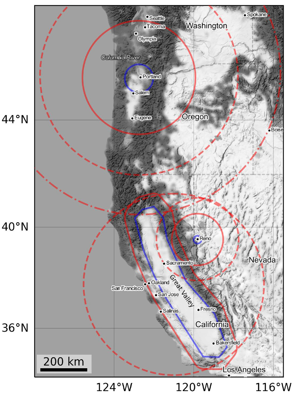
Earthquake (red) and station (blue) selection regions for the Great Valley, Reno, and Portland data sets. For each region, we use multiple search criteria for the earthquakes and one search criterion for the stations (refer to Tables 1 to 3). Map tiles by Stamen Design, under Creative Commons Attribution 3.0 Unported. Data by OpenStreetMap, under Open Data Commons Open Database License.

Table 1.

Earthquake and station selection parameters for the Great Valley

Data Type	Parameter	Value
	Region center a	121.00°W, 37.68°N
All earthquakes b	Start date	2000-01-01
	End date	2022-12-31
	Min. origin time separation	480 s
Smaller earthquakes	Min. magnitude	3.5
	Max. distance	Within 0.5° of station polygon
Larger earthquakes	Min. magnitude	4.5
	Max. distance	3.6°
Stations c	Max. distance	3.4°
	Data centers d	NCEDC, IRIS

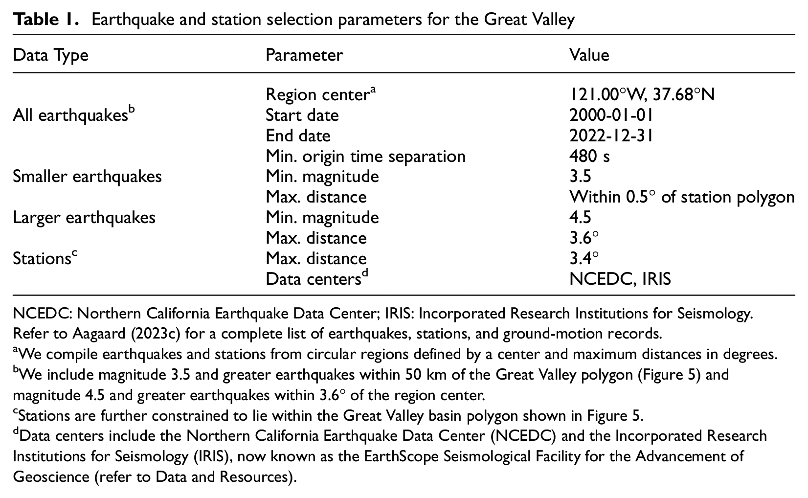
NCEDC: Northern California Earthquake Data Center; IRIS: Incorporated Research Institutions for Seismology.

Refer to Aagaard (2023c) for a complete list of earthquakes, stations, and ground-motion records.

a

We compile earthquakes and stations from circular regions defined by a center and maximum distances in degrees.

b

We include magnitude 3.5 and greater earthquakes within 50 km of the Great Valley polygon (Figure 5) and magnitude 4.5 and greater earthquakes within 3.6° of the region center.

c

Stations are further constrained to lie within the Great Valley basin polygon shown in Figure 5.

d

Data centers include the Northern California Earthquake Data Center (NCEDC) and the Incorporated Research Institutions for Seismology (IRIS), now known as the EarthScope Seismological Facility for the Advancement of Geoscience (refer to Data and Resources).

Table 2.

Earthquake and station selection parameters for Reno

Data Type	Parameter	Value
	Region center a	119.81°W, 39.52°N
All earthquakes b	Start date	2010-01-01
	End date	2022-12-31
	Min. origin time separation	60 s
Smaller earthquakes	Min. magnitude	3.0
	Max. distance	1.0°
Larger earthquakes	Min. magnitude	4.5
	Max. distance	1.6°
Stations	Max. distance	0.15°
	Data centers c	NCEDC, IRIS

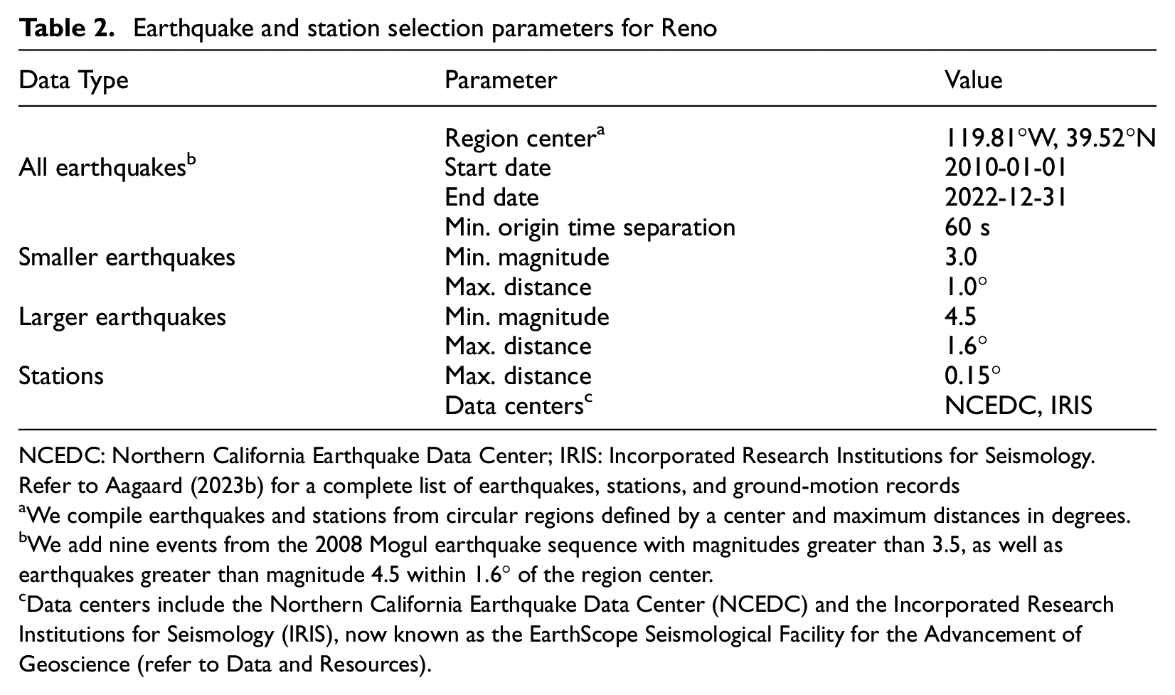
NCEDC: Northern California Earthquake Data Center; IRIS: Incorporated Research Institutions for Seismology.

Refer to Aagaard (2023b) for a complete list of earthquakes, stations, and ground-motion records

a

We compile earthquakes and stations from circular regions defined by a center and maximum distances in degrees.

b

We add nine events from the 2008 Mogul earthquake sequence with magnitudes greater than 3.5, as well as earthquakes greater than magnitude 4.5 within 1.6° of the region center.

c

Data centers include the Northern California Earthquake Data Center (NCEDC) and the Incorporated Research Institutions for Seismology (IRIS), now known as the EarthScope Seismological Facility for the Advancement of Geoscience (refer to Data and Resources).

Table 3.

Earthquake and station selection parameters for Portland

Data Type	Parameter	Value
	Region center a	122.75°W, 45.48°N
All earthquakes b	Start date	2005-11-01
	End date	2022-12-31
	Min. origin time separation	60 s
Smaller earthquakes	Min. magnitude	3.0
	Max. distance	2.0°
Moderate earthquakes	Min. magnitude	4.0
	Max. distance	3.5°
Larger earthquakes	Min. magnitude	5.5
	Max. distance	5.0°
Stations	Max. distance	0.5°
	Data centers c	IRIS

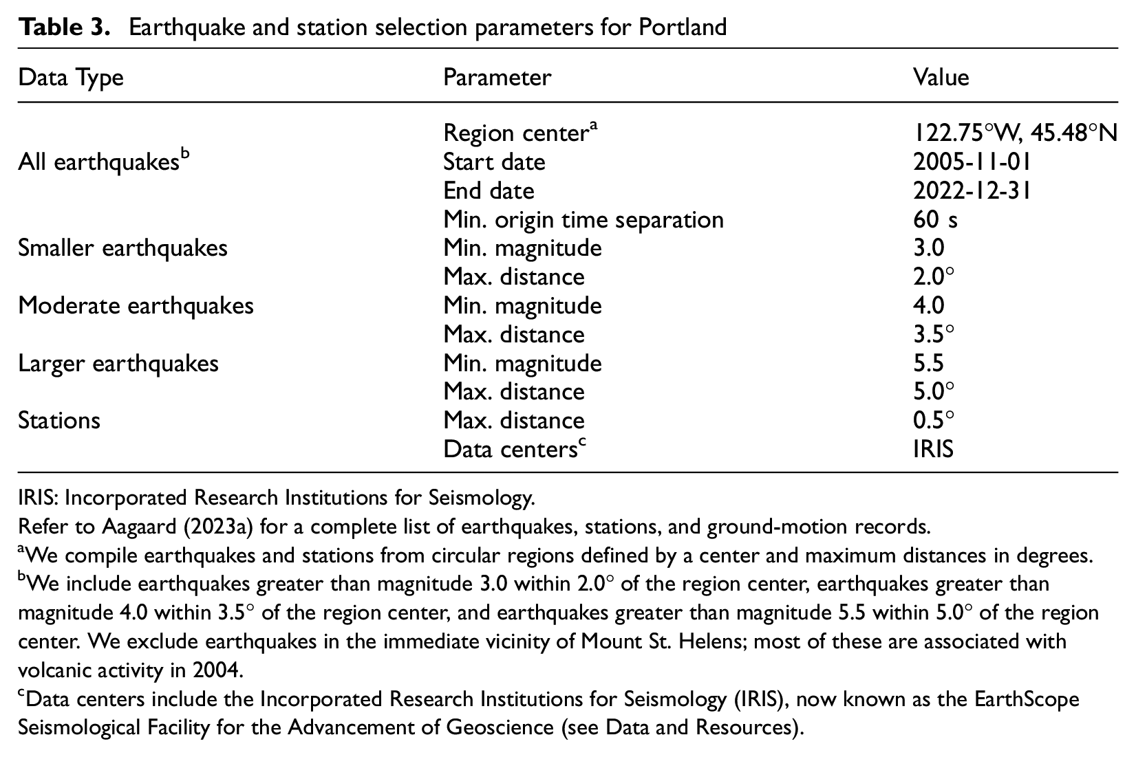
IRIS: Incorporated Research Institutions for Seismology.

Refer to Aagaard (2023a) for a complete list of earthquakes, stations, and ground-motion records.

a

We compile earthquakes and stations from circular regions defined by a center and maximum distances in degrees.

b

We include earthquakes greater than magnitude 3.0 within 2.0° of the region center, earthquakes greater than magnitude 4.0 within 3.5° of the region center, and earthquakes greater than magnitude 5.5 within 5.0° of the region center. We exclude earthquakes in the immediate vicinity of Mount St. Helens; most of these are associated with volcanic activity in 2004.

c

Data centers include the Incorporated Research Institutions for Seismology (IRIS), now known as the EarthScope Seismological Facility for the Advancement of Geoscience (see Data and Resources).

Ground-motion processing

We process the ground-motion waveforms using gmprocess (Hearne et al., 2019; version 1.2.3) to produce a file with each row containing earthquake information, station metadata and metrics, and intensity metrics for each ground-motion record. As part of the post-processing, we append local site information (V_S30, Z_1.0, and Z_2.5) and consolidate any collocated stations. The electronic supplement includes additional description of the data compilation and processing.

We use the default gmprocess processing steps, quality checks, and parameters. The processing steps include

1. Linear baseline correction;

2. Removal of instrument response;

3. Bandpass filtering with corner frequencies determined by the signal-to-noise ratio;

4. Duration trimming; and

5. Sixth-order polynomial baseline correction.

Aagaard (2023a, 2023b, 2023c) provide the raw and processed waveforms, ground-motion metrics, and basin-depth models for Portland, Oregon; Reno, Nevada; and the California Great Valley, respectively. Quality checks include verifying the presence of all three components and a minimum number of zero crossings, checking for clipping (Kleckner et al., 2022), and ensuring that the velocities and displacements at the end of the records are below a specified threshold. We also apply spectral period-specific filters to remove records that have total residuals greater than ±4 ln units (a factor of ∼55).

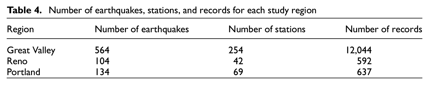
Table 4 shows the number of earthquakes, stations, and records for each region. Figures 2 to 4 show the number of records with spectral acceleration values at each period, the earthquake magnitude and distance parameter space, and the basin depth (Z_X) and V_S30 values at the stations. The Great Valley data set is much larger than the others due to its large geographic footprint, the presence of several permanent and temporary seismic networks, and a higher rate of seismicity. As mentioned previously, the Portland data set includes earthquakes at greater distances to increase the number of records at periods greater than 2.0 s.

Table 4.

Number of earthquakes, stations, and records for each study region

Region	Number of earthquakes	Number of stations	Number of records
Great Valley	564	254	12,044
Reno	104	42	592
Portland	134	69	637

Figure 2.

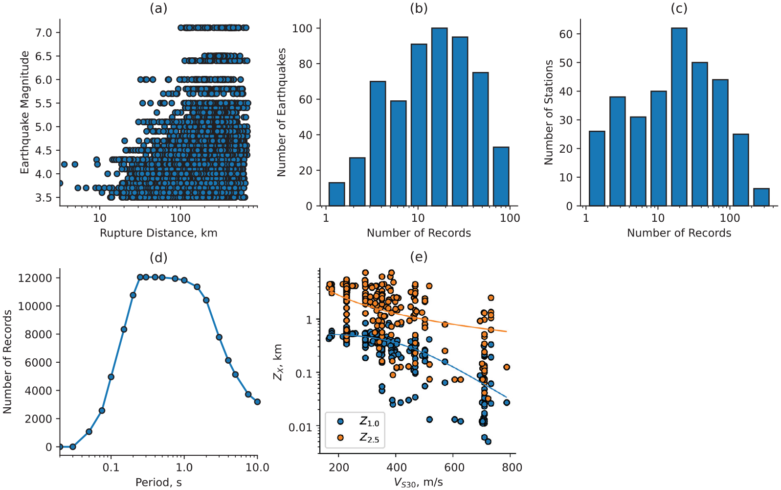
Characteristics of the California Great Valley ground-motion data set. (a) Earthquake magnitude versus distance for each ground-motion record, (b) histogram of the number of records for each earthquake, (c) histogram of the number of records for each station, (d) number of ground-motion records per spectral acceleration (SA) period, (e) depth to the 1.0 and 2.5 km/s shear-wave speed isosurfaces (Z_1.0 and Z_2.5, respectively) versus V_S30 (time-averaged shear-wave speed in the top 30 m) for each station; the solid lines correspond to the default Z_1.0 and Z_2.5 relations as a function of V_S30 from Boore et al. (2014) and Campbell and Bozorgnia (2014), respectively. Inclusion of broadband seismometers increases the bandwidth of the processed ground-motion records.

Figure 3.

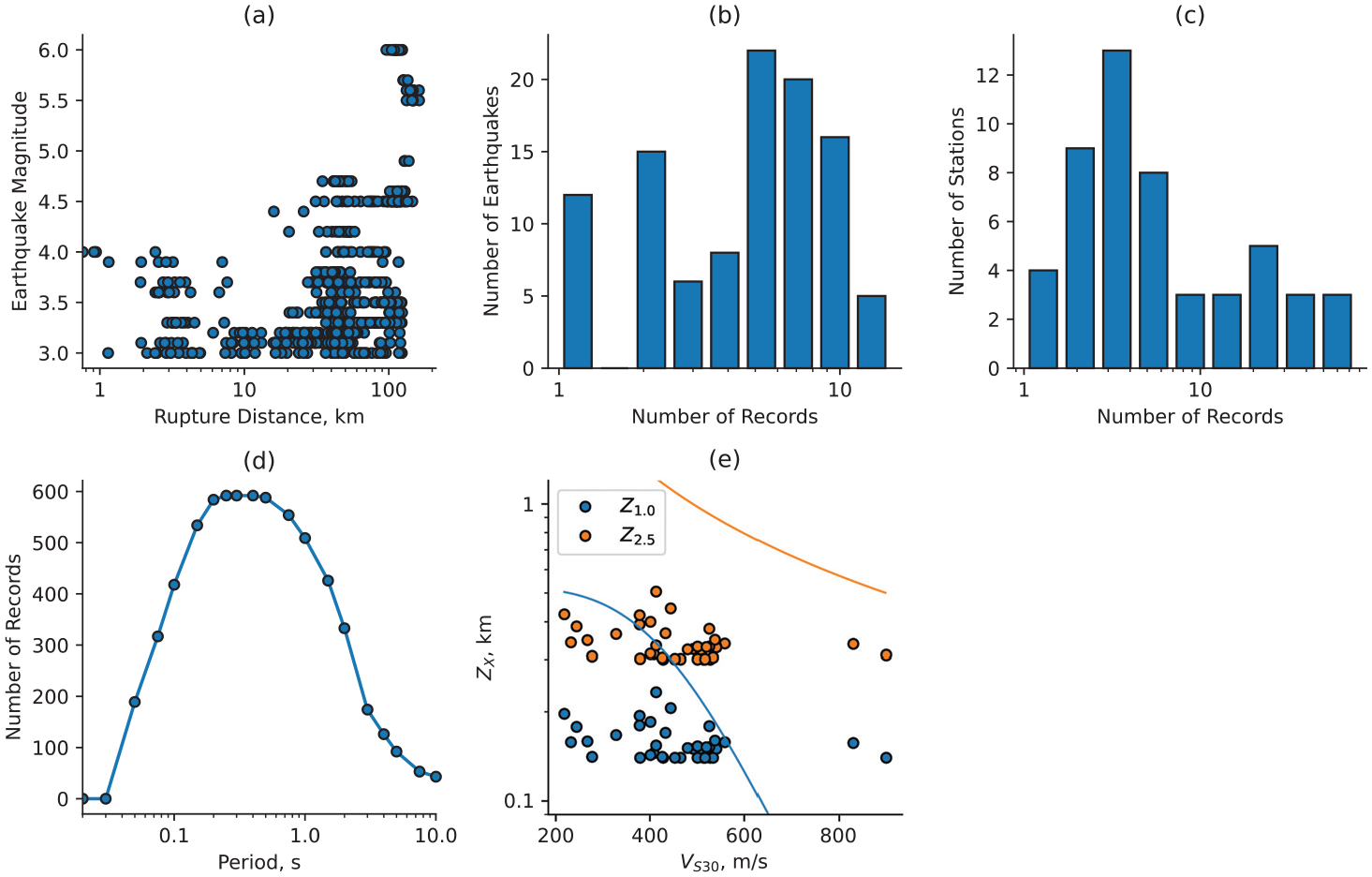
Characteristics of the Reno, Nevada, ground-motion data set. (a) Earthquake magnitude versus distance for each ground-motion record, (b) histogram of the number of records for each earthquake, (c) histogram of the number of records for each station, (d) number of ground-motion records per spectral acceleration (SA) period, (e) Z_1.0 and Z_2.5 versus V_S30 for each station; the solid lines correspond to the default Z_1.0 and Z_2.5 relations as a function of V_S30 from Boore et al. (2014) and Campbell and Bozorgnia (2014), respectively.

Figure 4.

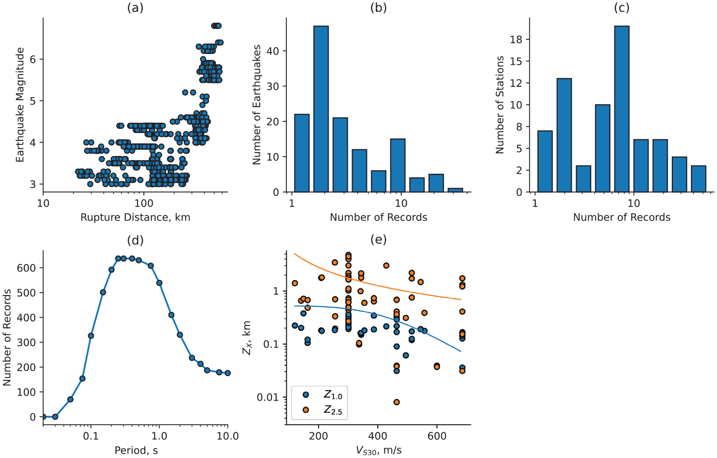
Characteristics of the Portland, Oregon, ground-motion data set. (a) Earthquake magnitude versus distance for each ground-motion record, (b) histogram of the number of records for each earthquake, (c) histogram of the number of records for each station, (d) number of ground-motion records per spectral acceleration (SA) period, (e) Z_1.0 and Z_2.5 versus V_S30 for each station; the solid lines correspond to the default Z_1.0 and Z_2.5 relations as a function of V_S30 from Boore et al. (2014) and Campbell and Bozorgnia (2014), respectively.

Discarding records with peak horizontal ground acceleration (PGA) >0.1 g to avoid nonlinear soil response eliminates three records in the Great Valley and four records in Reno.

Assignment of site-specific metadata

Shallow shear-wave velocity, V_S30

To ensure uniform quality of site condition parameters within a given region of interest, we use the mapped proxy-based V_S30 models from Thompson (2022) for the Great Valley and from the USGS Global V_S30 Mosaic (Heath et al., 2020) for Reno and Portland, the latter of which draws from the primary global topographic slope–based model of Wald and Allen (2007) and Allen and Wald (2009). We acknowledge that best practices require site-specific measurement of V_S30 at recording stations for the most accurate modeling of ground motions and site response. However, such measurements are not available at most seismic stations (Huddleston et al., 2021).

Candidate basin-depth models and Z_X

We discretize each regional Z_X model on a 0.01 degree-resolution raster grid. We use the Z_X values corresponding to the pixel in the raster grid containing the location of each seismic station in our analysis.

Great Valley

We create Z_X models for the Great Valley (Aagaard, 2023c) from a combination of the USGS San Francisco Bay region 3D seismic velocity model version 21.1 (SF-CVM, Aagaard and Hirakawa, 2021) and the USGS National Crustal Model (NCM) for seismic hazard studies version 220311 (Boyd and Shah, 2018). Both of these geologic-based seismic velocity models yield similar Z_X values. The SF-CVM model is simpler and the Z_X values are more uniform. We also considered using Z_X values from the SCEC CCA06 (https://github.com/SCECcode/cca) and the CVM-H v15.10 (Shaw et al., 2015) seismic velocity models, but both models have insufficient resolution in the top kilometer to provide reasonable Z_1.0 values; in addition, the Z_2.5 values in the CCA06 model are poorly correlated with basin depth as a result of introducing short length-scale velocity perturbations driven by full-waveform tomography.

We extract Z_X values from the SF-CVM and NCM models on a longitude and latitude grid at a uniform resolution of 0.01 degree. The SF-CVM includes only the northern three-quarters of the Great Valley, whereas the NCM includes the entire Great Valley. In the region where the two models overlap, we use the arithmetic average of the two models:

$$Z_X^{\mathrm{avg}}=\frac{1}{2}(Z_X^{\mathrm{SF}-\mathrm{CVM}}+Z_X^{\mathrm{NCM}}).$$

(3)

In the region where we only have values from the NCM, we want to use values consistent with the average value computed where the two models overlap. In the overlap region, we compute an average scaling factor, C, for the average values relative to the NCM. In the region with values from only the NCM, we apply this scaling factor to the NCM values to compute values for our average models:

$$Z_X^{\mathrm{avg}}={\mathrm{CZ}}_X^{\mathrm{NCM}},$$

(4)

where we compute the average scaling factor, C, using the geometric mean of the ratio of the average model value to the NCM model values in the overlap region:

$$C=\exp \left(\mathrm{mean}\left(\log \left({\mathrm{Z}}_{\mathrm{X}}^{\mathrm{avg}}/{\mathrm{Z}}_{\mathrm{X}}^{\mathrm{NCM}}\right)\right)\right).$$

(5)

We compute the geometric mean using exponential and logarithm functions and the arithmetic mean across all points within the overlap region. The SF-CVM and NCM Z_X values are quite close, so the scaling factor C is close to 1.0. For Z_1.0, C is 1.10 and for Z_2.5, C is 1.00. Figure 5 shows the Great Valley Z_X models.

Figure 5.

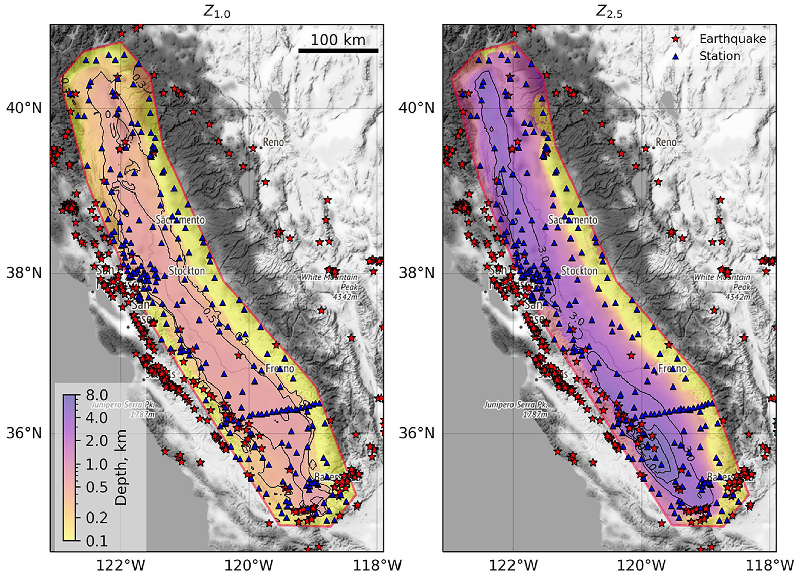
Maps of Z_1.0 and Z_2.5 (depths of the 1.0 and 2.5 km/s shear-wave speed isosurfaces) for the Great Valley in California. The thin black lines show contours of Z_X at depths of 0.3, 0.5, 0.7 km for Z_1.0 and 3.0, 5.0, and 7.0 km for Z_2.5. The red stars indicate earthquakes producing ground-motion records at the stations shown by blue triangles; some earthquakes lie outside the map region and not all earthquakes have records at all stations. The red polygon defines the candidate region for using the Z_X models in the National Seismic Hazard Model. Legend in left panel applies to both panels. Map tiles by Stamen Design, under Creative Commons Attribution 3.0 Unported. Data by OpenStreetMap, under Open Data Commons Open Database License.

Reno

The candidate Z_X models for Reno come from Simpson and Louie (2020), who utilize a database of V_S30 measurements derived from the Refraction Microtremor method (ReMi^TM; Louie, 2001), a passive-source surface-wave geophysical method used to model V_S. 170 ReMi measurements in the Reno area are correlated with background gravity surveys of Saltus and Jachens (1995) and Abbott and Louie (2000), which are used to estimate Z_X across the study region. The Reno area (Figure 6) includes Z_1.0 values ranging from 0.14 to 0.25 km and Z_2.5 values ranging from 0.30 to 0.54 km; stations in the data set have maximum assigned Z_1.0 and Z_2.5 of 0.23 and 0.51 km, respectively. We attribute the limited spatial variation in Z_1.0 and Z_2.5 in the Reno basin to thin sediments overlying shallow (∼0.5 km) tertiary volcanic rock overlying Mesozoic granites and metavolcanic rocks (Pancha et al., 2017; Simpson and Louie, 2020).

Figure 6.

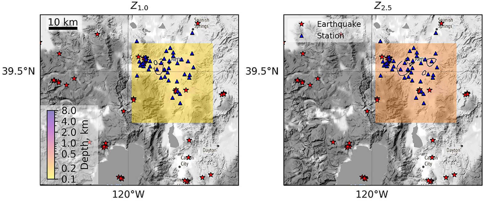
Maps of Z_1.0 and Z_2.5 (depths of the 1.0 and 2.5 km/s shear-wave speed isosurfaces) for the Reno, Nevada, area. The thin black lines show contours of Z_X at depths of 0.2 km for Z_1.0 and 0.4 km for Z_2.5. The red stars indicate earthquakes producing ground-motion records at the stations shown by blue triangles; some earthquakes lie outside the map region and not all earthquakes have records at all stations. Map tiles by Stamen Design, under Creative Commons Attribution 3.0 Unported. Data by OpenStreetMap, under Open Data Commons Open Database License.

Portland

The candidate Z_X models for Portland (Aagaard, 2023a) are derived from the NCM (Boyd and Shah, 2018) version 221024. Z_1.0 generally coincides with the top of the Columbia River Basalt Group as mapped by Scanlon et al. (2021), a geologically recent Tertiary lava flow that has a strong impedance contrast with the overlying younger sediments. Z_2.5 in this region of the NCM is highly variable. We therefore assume that Z_2.5 coincides with the top of the early tertiary basement rock, as modeled in a gravity study by McPhee et al. (2014) and compiled in Scanlon et al. (2021). In the NCM, this surface is defined by the regional work of Mooney and Kaban (2010) with a smooth transition to the model of McPhee et al. (2014) in the Portland area. The Portland area (Figure 7) includes Z_1.0 values ranging from 0 to 0.40 km and Z_2.5 values ranging from 0 to 4.6 km.

Figure 7.

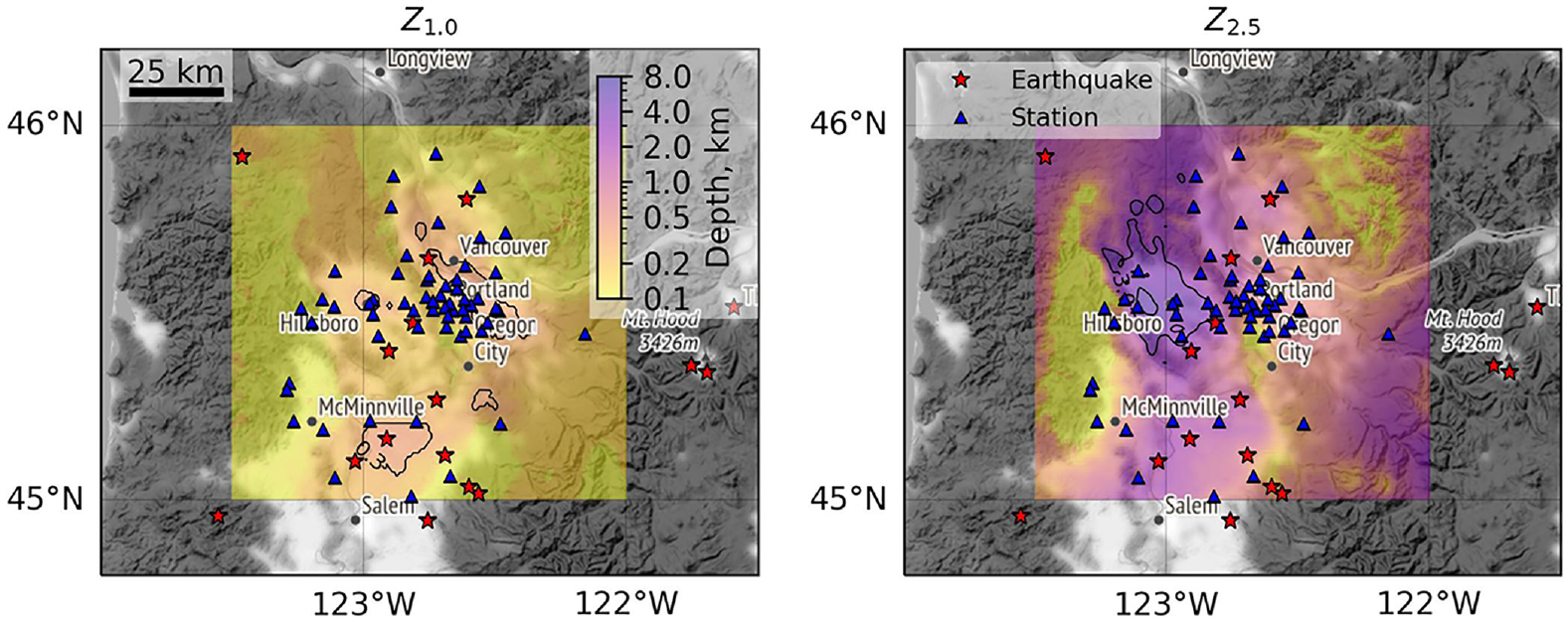
Maps of Z_1.0 and Z_2.5 (depths of the 1.0 and 2.5 km/s shear-wave speed isosurfaces) for the Portland, Oregon, area. The thin black lines show contours of Z_X at depths of 0.3 km for Z_1.0 and 3.0 and 5.0 km for Z_2.5. The Z_2.5 = 3.0 km contour just east of Hillsboro outlines the Tualatin basin and the Z_1.0 = 0.3 km contour just east of Portland and south of Vancouver outlines the Portland basin. The red stars indicate earthquakes producing ground-motion records at the stations shown by blue triangles; some earthquakes lie outside the map region and not all earthquakes have records at all stations. Map tiles by Stamen Design, under Creative Commons Attribution 3.0 Unported. Data by OpenStreetMap, under Open Data Commons Open Database License.

Ground-motion residuals analysis

Ground-motion residuals, R, are defined as the natural logarithmic difference between an observed IM (Y_OBS) and a GMM prediction (Y_GMM) using the generalized equation:

$$R=\ln \left(Y_{\mathrm{OBS}}\right)-\ln \left(Y_{\mathrm{GMM}}\right).$$

(6)

The evaluation of Y_GMM requires input parameters related to the earthquake source (i.e., magnitude) and path effects (e.g., source-to-recording-site distance). We are primarily interested in the site and basin components of these GMMs and how variation of those components affects the residuals. In this study, which investigates candidate Z_X model performance and the applicability of particular GMMs to target regions, we define two sets of residuals:

1. Total Residuals (R_T), computed using site-specific V_S30 and values from candidate Z_X models:

   $$R_T=\ln \left(Y_{\mathrm{OBS}}\right)-\ln \left[Y_{\mathrm{GMM}}(V_{S30},Z_X)\right].$$
   (7)

2. Total Residuals with default Z_X (R_T,def), computed using site-specific V_S30 and default Z_X values computed for each GMM as a function of V_S30:

   $$R_{T,\mathrm{def}}=\ln \left(Y_{\mathrm{OBS}}\right)-\ln \{Y_{\mathrm{GMM}}[V_{S30},Z_X=Z_X\left(V_{S30}\right)]\}.$$
   (8)

We omit the nonlinear site response term in computing the residuals because the data sets are composed of recordings of predominantly small-to-moderate magnitude events or large events at far-field distances. To check the validity of this assumption, we compare PGA with the criteria of Beresnev and Wen (1996), who estimate that nonlinearity may be present for PGA > 0.1 g. In our study, only three records in the Great Valley and four records in Reno exceed this threshold, and we discard these records from our analysis.

We follow the conventions of Parker and Baltay (2022) to assess site-specific response by partitioning these sets of residuals using mixed-effects regressions (Abrahamson and Youngs, 1992; Bates et al., 2015; R Core Team, 2020). We investigate trends in portions of the ground motions that are attributable to different predictor variables. The partitioning of the residuals yields a fixed effect, k, which represents an overall estimate of GMM bias for the given regional data set; event terms (δE_i) and site-to-site residuals (δS2S_j), which depend on grouping factors (event i and station j) and represent repeatable effects; and a remaining residual ε_ij (Al Atik et al., 2010). We start by partitioning the total residuals R_T as:

$$R_{T,\mathrm{ij}}=k+\delta E_i+\delta S2S_j+{\epsilon }_{\mathrm{ij}}.$$

(9)

We compute within-event residuals (WIER) by subtracting the event terms from each set of total residuals (R_T,ij and R_T,def,ij), thus removing the bias related to a specific event and leaving the variable station-to-station component, plus a remaining, unexplained residual. We compute two types of WIERs:

1. Total WIER (δW_T,ij), computed from R_T using site-specific V_S30 and values from candidate Z_X models:

   $$\delta W_{T,\mathrm{ij}}=R_{T,\mathrm{ij}}-\delta E_i-k=\delta S2S_j+{\epsilon }_{\mathrm{ij}}.$$
   (10)

2. Total WIER with default Z_X (δW_T,def,ij), computed from R_T,def using site-specific V_S30 and default Z_X values computed for each GMM as a function of V_S30:

$$\delta W_{T,\mathrm{def},\mathrm{ij}}=R_{T,\mathrm{def},\mathrm{ij}}-\delta E_i-k=\delta S2S_{j,\mathrm{def}}+{\epsilon }_{\mathrm{ij}}.$$

(11)

The δS2S_j and δS2S_j,def provide site-specific estimates of the portion of recorded ground motion attributed to linear site response that is not modeled by the GMM (either with the site-specific Z_X or the GMM-specific default value, respectively). The ε_ij represents any remaining effects not modeled by the GMM, which includes path-to-path variations in ground-motion attenuation or event-to-event variations in site response.

Analysis of ground-motion scaling in individual basins

Our primary goal is to use recorded ground motions to ascertain whether local Z_X values in a target region improve ground-motion predictions relative to default Z_X values (i.e., GMMs without basin terms). We examine residuals and assess whether the existing basin terms in BSSA14 and CB14 (as parameterized by δZ_1.0 and Z_2.5, respectively) effectively describe the observed basin amplification in a target region. That is, we assess whether the GMM basin terms match the trends of within-event total residuals computed with the default Z_X parameters for the GMM (δW_T,def). We also quantify changes to the accuracy of the ground-motion predictions as captured by the mean WIER and standard deviation of site-to-site residuals (denoted ϕ _S2S ) when using local Z_X models compared to default Z_X values. Variations of WIER and δS2S with predictor variables such as V_S30 and Z_X are expected to be similar, but the standard deviation of WIER (ϕ) is usually dominated by repeatable path effects, so comparing ϕ _S2S is more useful for our Z_X analyses.

The BSSA14 basin term, $F_{\delta Z_{1.0}}$ , is defined as:

$$F_{\delta Z_{1.0}}\left(\delta Z_{1.0}\right)=\{\begin{array}{c}0\hfill \\ \multicolumn{1}{c}{f_6\delta Z_{1.0}}\\ \multicolumn{1}{c}{f_7}\end{array}\begin{array}{c}T<0.65\hfill \\ \multicolumn{1}{c}{T\ge 0.65\mathrm{and}\delta Z_{1.0}\le f_7/f_6}\\ \multicolumn{1}{c}{T\ge 0.65\mathrm{and}\delta Z_{1.0}>f_7/f_6,}\end{array}$$

(12)

where f₆ and f₇ are the model coefficients, f₇/f₆ has units of km, and δZ_1.0 (also in km) is defined in Equation 1, (our notation differs slightly from that of BSSA14). The CB14 basin term (using our notation), f_sed, is defined as:

$$f_{\mathrm{sed}}\left(Z_{2.5}\right)=\{\begin{array}{c}{c}_{14}(Z_{2.5}-1)\hfill \\ \multicolumn{1}{c}{0}\\ \multicolumn{1}{c}{c_{16}{k}_3{e}^{-0.75}(1-\exp (-0.25(Z_{2.5}-3\mathrm{km})))}\end{array}\begin{array}{c}{Z}_{2.5}<1\hfill \\ \multicolumn{1}{c}{1\le Z_{2.5}\le 3}\\ \multicolumn{1}{c}{Z_{2.5}>3,}\end{array}$$

(13)

where $c_{14}$ , $c_{16}$ , and $k_3$ are the model coefficients. In the following sections, we discuss this residuals analysis and place emphasis on long periods (T > 1.0 s), which are of greatest interest for deeper sedimentary deposits.

Great Valley, California

The Great Valley has the richest ground-motion data set of the three target regions, providing the best constraints on basin response, particularly at long periods. The Great Valley is a long and deep sedimentary basin, with maximum values of Z_1.0 and Z_2.5 reaching 0.90 and 7.4 km, respectively, in the southwest portion of the basin (Aagaard, 2023c). The deepest Z_X values assigned to stations within our data set are 0.84 and 7.4 km for Z_1.0 and Z_2.5, respectively. Most stations (and ground-motion records) in the Great Valley (Figure 8) are concentrated within the range −0.2 < δZ_1.0 < 0.2: only 7% of stations in the data set fall outside this range.

Figure 8.

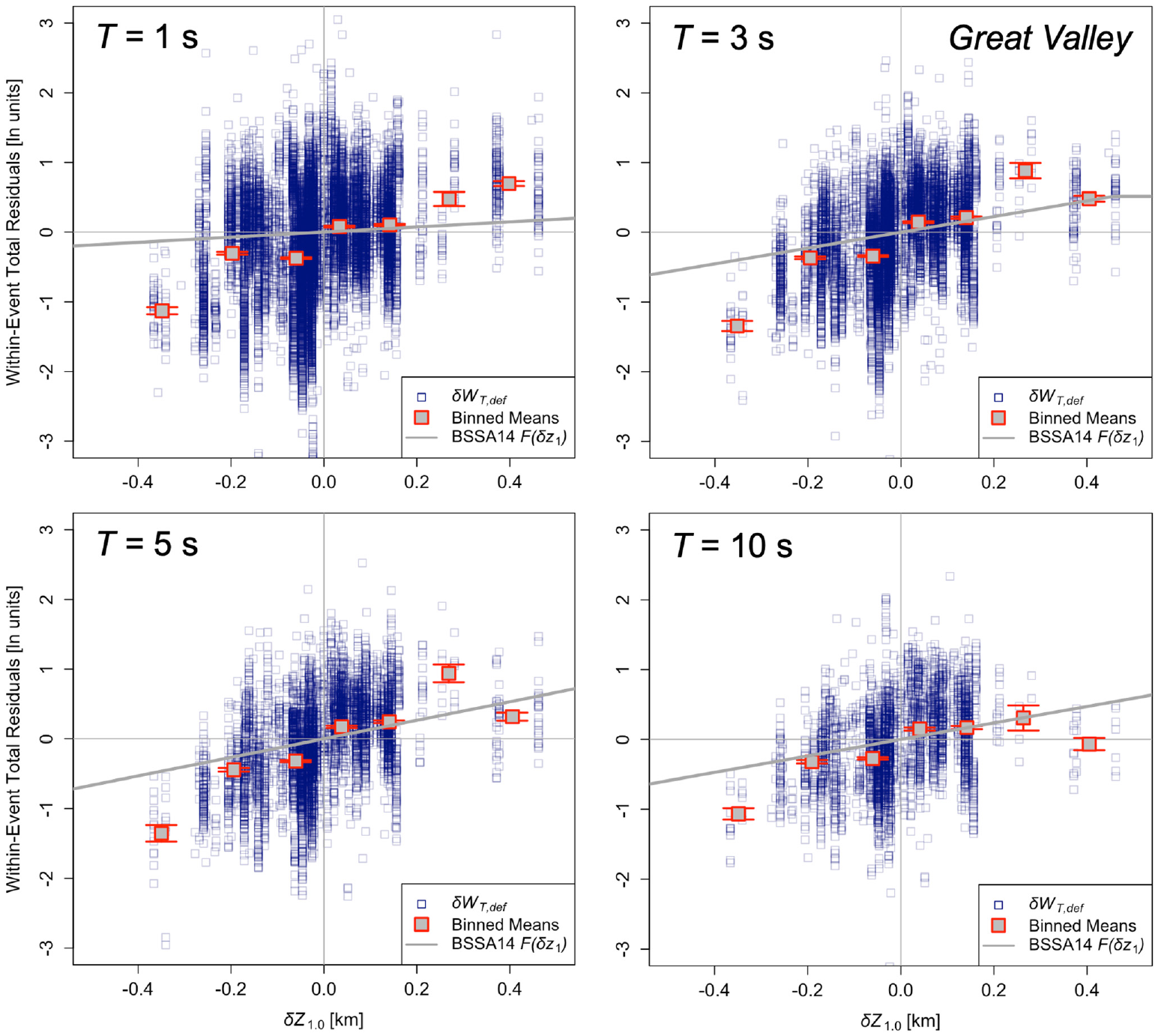
Empirical basin-depth scaling in the California Great Valley as a function of δZ_1.0 (Equation 1) using the Boore et al. (2014; BSSA14) ground-motion model for four oscillator periods of interest (T = 1.0, 3.0, 5.0, and 10 s). The rectangles denote the total within-event residuals for default V_S30-based Z_X values (δW_T,def) as well as the binned mean values and their standard deviations. The electronic supplement includes plots for ten oscillator periods between 0.5 and 10 s (Supplemental Figure S1).

Binned means of δW_T,def closely follow the period-specific basin-amplification functions of BSSA14, as was expected given the California-centric data set used to develop the NGA-West2 models. Outside of the range −0.2 < δZ_1.0 < 0.2, the agreement is poorer with substantial deamplification for the observed ground motions compared to the basin terms; however, this is a small fraction of the data. For CB14, binned means of δW_T,def tend to be slightly larger than the GMM prediction (more amplification, Figure 9) for Z_2.5 of 5 km but slightly smaller (greater deamplification) for Z_2.5 in the range of 0.1–0.5 km. Plots showing the correlation of site-to-site residuals (δS2S_j) to Z_X (Figures S7 and S8 in the electronic supplement) show similar trends to WIER data presented in Figures 8 and 9 and comprise the data summarized in Table 5.

Figure 9.

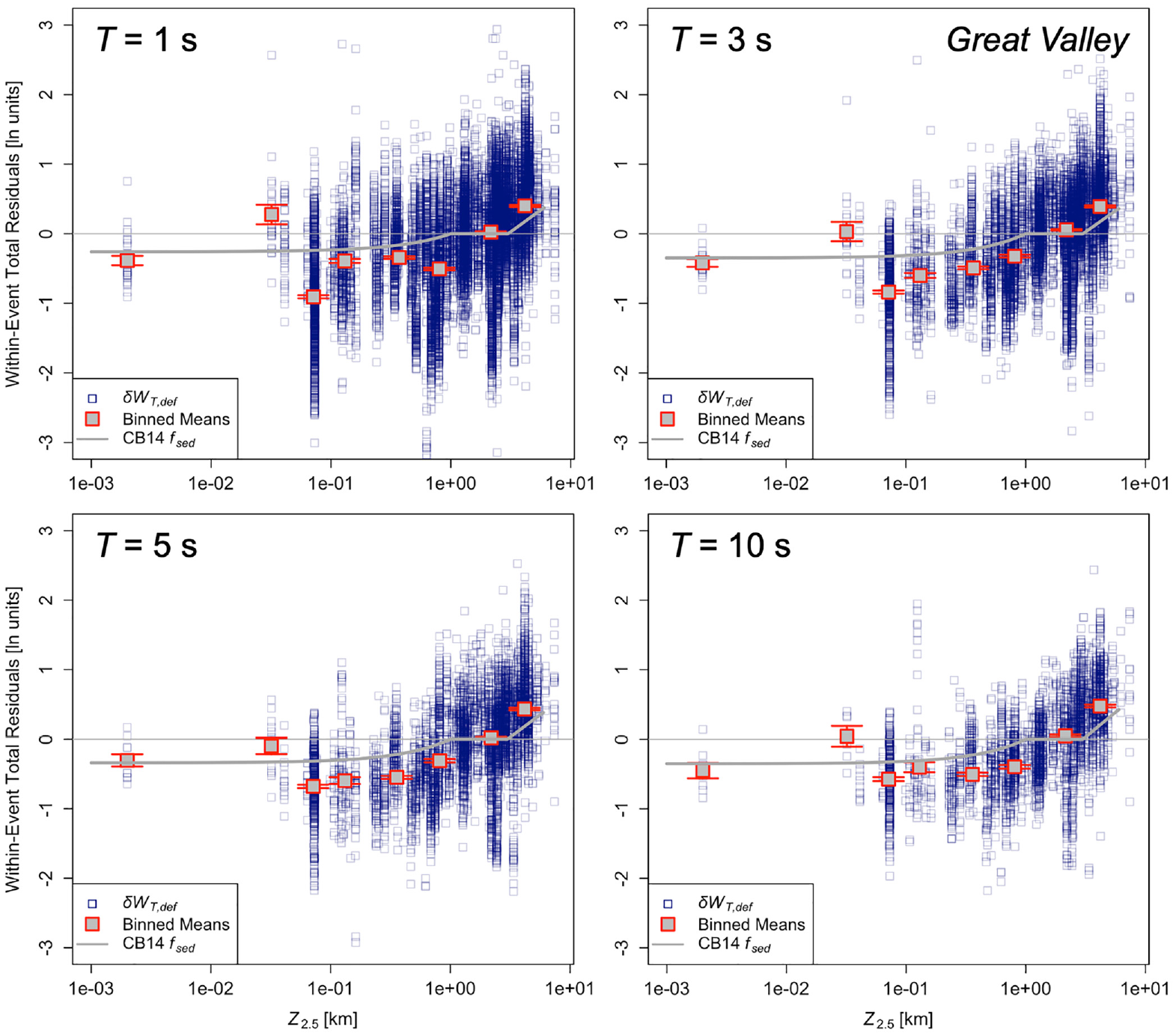
Empirical basin-depth scaling in the California Great Valley as a function of Z_2.5 relative to the Campbell and Bozorgnia (2014; CB14) ground-motion model for four oscillator periods of interest (T = 1.0, 3.0, 5.0, and 10 s). The rectangles denote the total within-event residuals for default V_S30-based Z_X values (δW_T,def) as well as the binned mean values and their standard deviations. The electronic supplement includes plots for ten oscillator periods between 0.5 and 10 s (Supplemental Figure S2).

Table 5.

Summary of changes in standard deviation of within-event residuals (Δϕ) across oscillator periods when using the local Z_X model (localZx) of Aagaard (2023c) over the NGA-West2 defaultV_S30-based Z_X model (defZx) in the California Great Valley

Period, T (s)	Z1.0			Z2.5
	ϕS2S,defZx	ϕS2S,localZx	ΔϕS2S (%)	ϕS2S,defZx	ϕS2S,localZx	ΔϕS2S (%)
1.0	0.62	0.61	−1.9	0.64	0.58	−9.3
1.5	0.62	0.59	−3.5	0.63	0.56	−11
2.0	0.61	0.58	−4.9	0.61	0.53	−13
3.0	0.59	0.55	−6.7	0.61	0.52	−14
4.0	0.59	0.54	−8.2	0.61	0.51	−16
5.0	0.59	0.53	−9.1	0.61	0.51	−16
7.5	0.58	0.53	−8.5	0.64	0.53	−17
10.	0.57	0.53	−6.3	0.59	0.49	−18

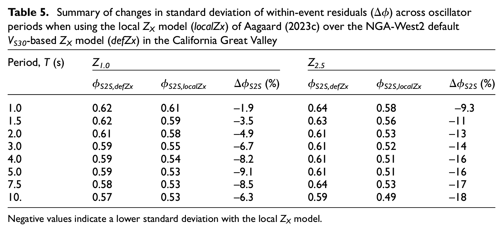
Negative values indicate a lower standard deviation with the local Z_X model.

BSSA14 and CB14 capture the overall trend, leading to a reduction in standard deviation of site-to-site residuals (ϕ _S2S ) for periods between 1.0 and 10 s (Table 5 and Supplemental Tables S1 and S2 and Figure 10). Using the Great Valley Z_1.0 yields a marginal reduction of 2%–9% for ϕ _S2S for the range 1 ≤ T ≤ 10 s, but a more appreciable reduction of 9%–18% of ϕ _S2S when using the local Z_2.5 model over the same period range.

Figure 10.

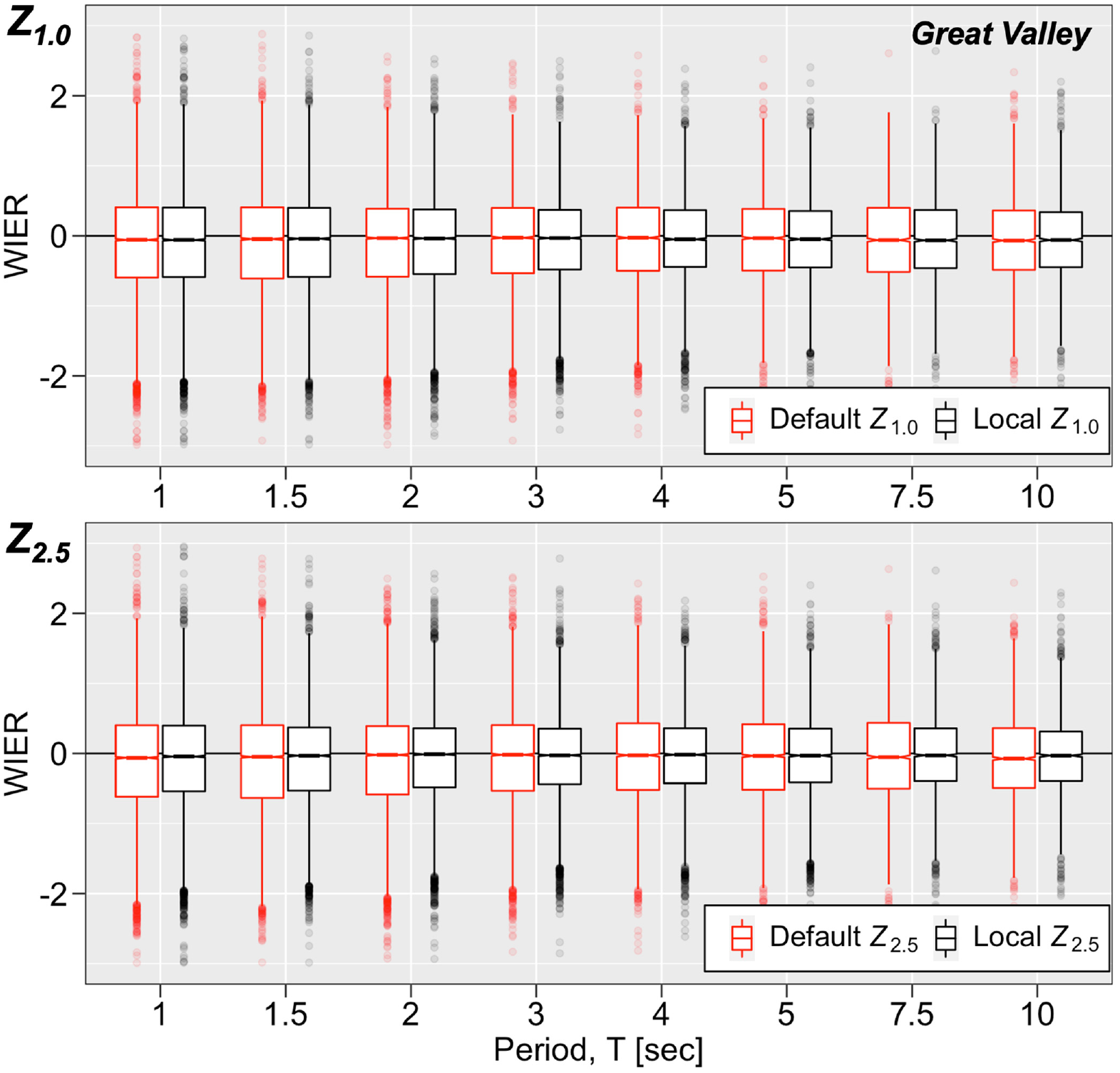
Boxplots showing change in mean values and standard deviations of within-event residuals (WIER) across oscillator periods when using the local Z_X model of Aagaard (2023c) over the NGA-West2 default V_S30-based Z_X model in the California Great Valley; top: Z_1.0, bottom: Z_2.5. The box delineates the 25th, 50th (median), and 75th percentiles, the vertical lines (whiskers) extend either direction to 1.5 times the inter-quartile range (IQR, the difference between the value and the 75th and 25th percentiles), and the outliers beyond the whiskers are represented with circular symbols. Notches in the boxplot (which are very small in this case) span the value of 1.58 times the IQR divided by the square root of the number of points, providing roughly a 95% confidence interval for comparing medians. Supplemental Tables S1 to S4 give the corresponding medians and standard deviations.

We estimate the contribution to epistemic uncertainty from the seismic velocity models, making use of the SF-CVM and NCM Z_X models that we used to compute the average Z_X model. Normally, we use δ as the symbol for uncertainty, but this conflicts with the use of relative basin depth $\delta Z_{1.0}$ ; consequently, we use ψ to denote uncertainty. For BSSA14, the site term, F_S (Equation 12), is proportional to the relative basin depth $\delta Z_{1.0}$ for T > 0.65 s and δZ_1.0 < f₇/f₆, so we have:

$$\mathrm{\psi }(\mathrm{FS})=\mathrm{\psi }(F_{\delta Z_{1.0}})=f_6\mathrm{\psi }(\delta Z_{1.0})\mathrm{for}T\ge 0.65s\mathrm{and}\delta Z_{1.0}<f_7/f_6,$$

(14)

where ψ (x) denotes the uncertainty in x; f₆ and f₇ are the model coefficients; and:

$$\mathrm{\psi }(\delta Z_{1.0})=\mathrm{\psi }(Z_{1.0}^{\mathrm{SF}-\mathrm{CVM}})+\mathrm{\psi }(Z_{1.0}^{\mathrm{NCM}}).$$

(15)

For CB14, the basin term (Equation 13) at depths greater than 3 km is a nonlinear function of Z_2.5:

$$f_{\mathrm{sed}}=c_{16}{k}_3{e}^{-0.75}(1-\exp (-0.25(Z_{2.5}-3)))\mathrm{for}{Z}_{2.5}>3\mathrm{km}.$$

(16)

We differentiate with respect to Z_2.5 to compute the uncertainty in f_sed, $\mathrm{\psi }(f_{\mathrm{sed}})$ , given the uncertainty in Z_2.5, $\mathrm{\psi }(Z_{2.5})$ , which yields:

$$\mathrm{\psi }(f_{\mathrm{sed}})=0.25c_{16}{k}_3\exp (-0.25Z_{2.5})\mathrm{\psi }(Z_{2.5})\mathrm{for}{Z}_{2.5}>3\mathrm{km},$$

(17)

where c₁₆ and k₃ are the model coefficients. We compute the uncertainty in Z_X using:

$$\mathrm{\psi }(Z_X)=\frac{1}{2}(\mathrm{\psi }\left(Z_X^{\mathrm{SF}-\mathrm{CVM}}\right)+\mathrm{\psi }\left(Z_X^{\mathrm{NCM}}\right))$$

(18)

$$\mathrm{\psi }\left(Z_X^{\mathrm{SF}-\mathrm{CVM}}\right)=\mathrm{std}(Z_X^{\mathrm{SF}-\mathrm{CVM}}-Z_X^{\mathrm{avg}})$$

(19)

$$\mathrm{\psi }(Z_X^{\mathrm{NCM}})=\mathrm{std}(Z_X^{\mathrm{NCM}}-Z_X^{\mathrm{avg}}),$$

(20)

where $Z_X^{\mathrm{SF}-\mathrm{CVM}}$ denotes Z_X in the SF-CVM 3D seismic velocity model, $Z_X^{\mathrm{NCM}}$ denotes Z_X in the NCM, $Z_X^{\mathrm{avg}}$ denotes our averaged Z_X from the SF-CVM and the NCM, and std(x) denotes the standard deviation of x. We find ψ( $\delta Z_{1.0}$ ) is 60 m and ψ(Z_2.5) is 500 m, where we compute ψ(Z_2.5) at Z_2.5 equal to 4.2 km, which is the average Z_2.5 value over the region where Z_2.5 ≥ 3 km. Figure 11 displays this estimate of epistemic uncertainty in F_S and f_sed as a function of period using these values. The epistemic uncertainty in the basin terms for BSSA14 and CB14 is both about 0.06–0.08 ln units at periods greater than 3.0 s. As a result of the functional forms chosen for the basin terms in the GMM and the model coefficients, the uncertainty in the basin term for BSSA14 decreases to 0 at a period of 0.65 s, whereas the uncertainty in the basin term for CB14 remains about 0.06 ln units.

Figure 11.

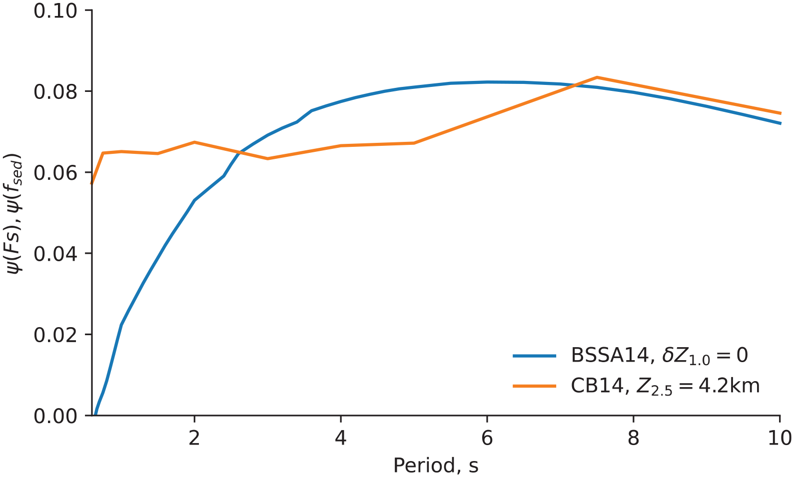
Estimate of epistemic uncertainty in the California Great Valley (Boore et al., 2014, BSSA14; and Campbell and Bozorgnia, 2014, CB14) basin terms (F_S and f_sed, respectively) as a function of period. The uncertainty in the BSSA14 F_S term is smaller at shorter periods, whereas the uncertainty in CB14 f_sed term is relatively constant across periods. The uncertainties are both about 0.06–0.08 ln units at periods greater than 3.0 s.

Reno, Nevada

Reno basin-depth models are relatively shallow compared to those in California used to develop the NGA-West2 GMMs. The basin term in BSSA14 predicts deamplification (δZ_1.0 < 0) at 44 of the 51 (86%) stations in our data set. The 2018 NSHM (Powers et al., 2021) did not allow such deamplification. Only four stations, comprising 16 ground-motion records, have δZ_1.0 > 0 (positive amplification relative to the V_S30-based default basin depth); these sites have Z_1.0 < 0.16 km and Z_2.5 < 0.54 km. Binned mean values of δW_T,def are relatively independent of the basin-amplification predictor variable δZ_1.0, especially at periods of 3.0 and 10 s (Figure 12). That is, the recorded ground motions exhibit less amplification and deamplification than that predicted by BSSA14. For CB14, the limited range of Z_2.5 and the scatter in the observed ground motion makes it difficult to assess whether the binned means are significantly correlated with the period-specific basin-amplification function (Figure 13).

Figure 12.

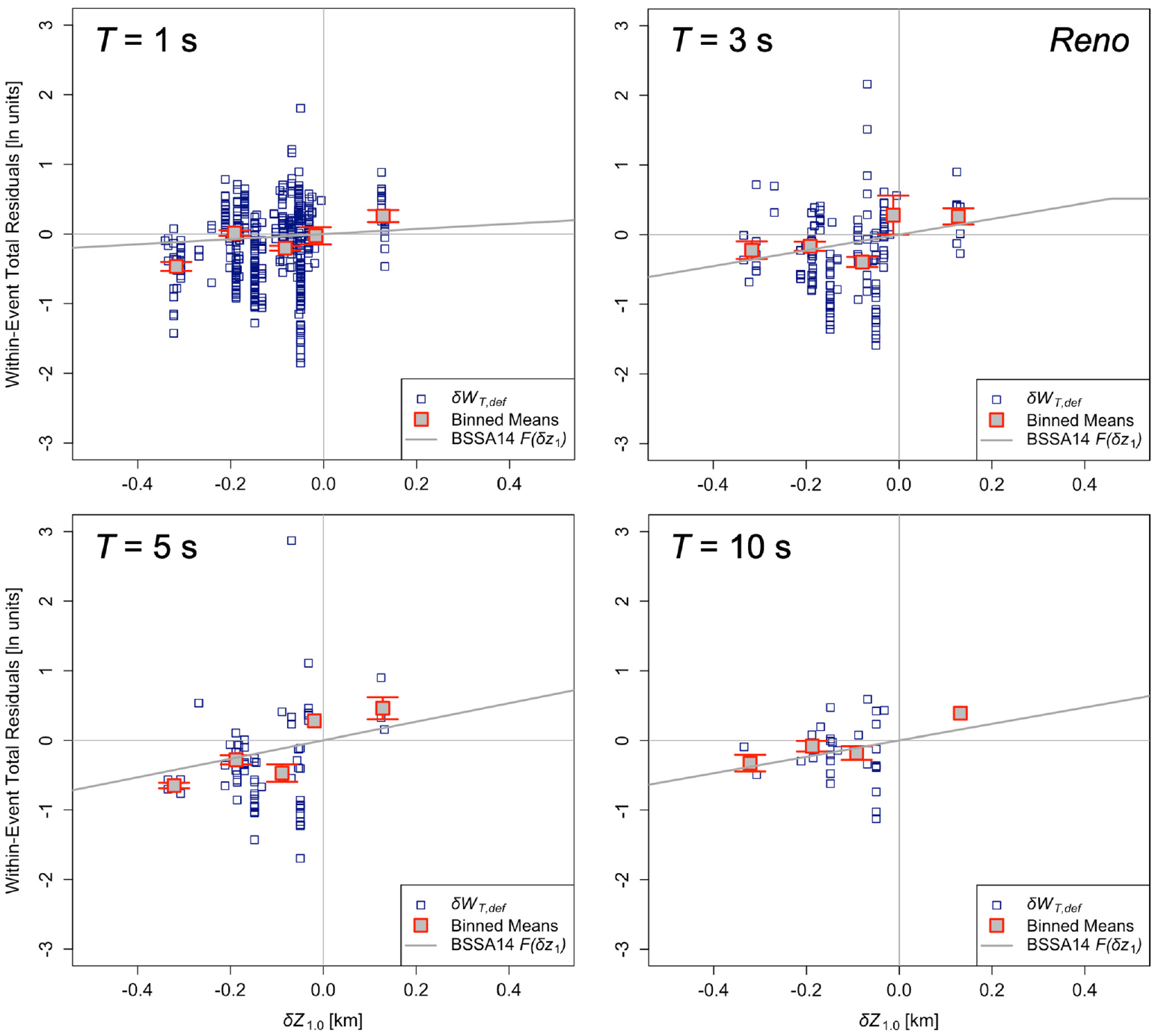
Empirical basin-depth scaling in Reno, Nevada as a function of δZ_1.0 (Equation 1) using the Boore et al. (2014; BSSA14) ground-motion model for four oscillator periods of interest (T = 1.0, 3.0, 5.0, and 10 s). The rectangles denote the total within-event residuals for default V_S30-based Z_X values (δW_T,def) and the binned mean values and standard deviations. The binned mean value on the T = 10 s plot includes and obscures only one data point, and thus, it has no error bars. The electronic supplement includes plots for ten oscillator periods between 0.5 and 10 s (Supplemental Figure S3).

Figure 13.

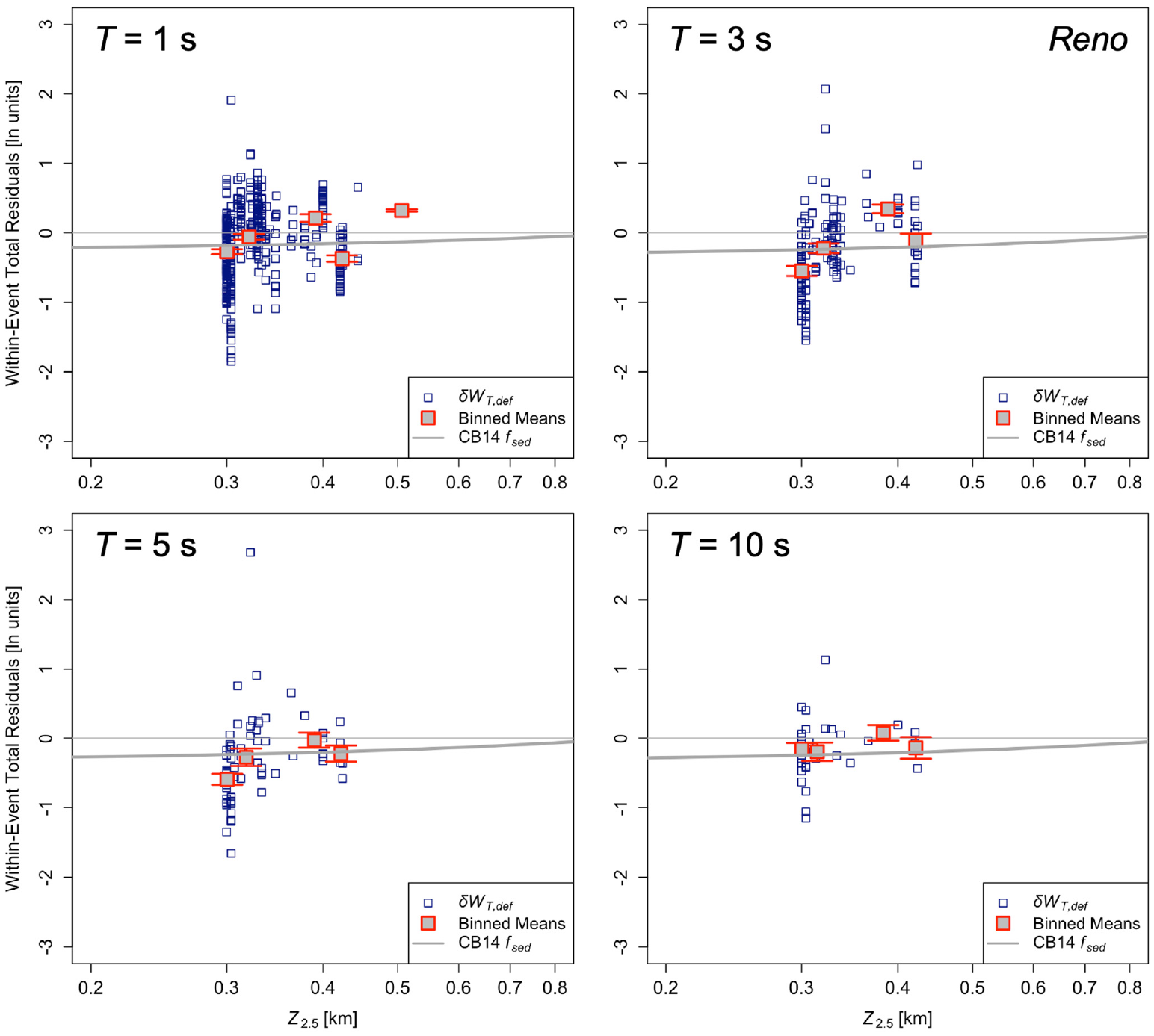
Empirical basin-depth scaling in Reno, Nevada, as a function of Z_2.5 using the Campbell and Bozorgnia (2014; CB14) ground-motion model for four oscillator periods of interest (T = 1.0, 3.0, 5.0, and 10 s). The rectangles denote the total within-event residuals for default V_S30-based Z_X values (δW_T,def) as well as the binned mean values and their standard deviations. Note difference in x-axis limits from Figure 9. The electronic supplement includes plots for ten oscillator periods between 0.5 and 10 s (Supplemental Figure S4).

Table 6 summarizes the standard deviation of δS2S (ϕ _S2S ) with and without the use of the local Z_X models in Reno. The use of the candidate Z_1.0 model yields a marginal reduction of less than 5% for ϕ _S2S for the range 1 ≤ T ≤ 3 s, with more appreciable reduction in ϕ _S2S of 6%–14% at longer periods. Improvements in ϕ _S2S range from 11% to 5% when using the local Z_2.5 model over the range 1 ≤ T ≤ 5 s but show more substantial improvements of up to 22% at the longest periods (7.5 and 10 s); however, the data set includes only 52 records from 26 stations at T = 7.5 s and 43 records from 21 stations at T = 10 s. Both default V_S30-based models and the candidate Z_X models, on average, overpredict the ground motions across all periods (Figure 14 and Supplemental Tables S5 and S6), perhaps reflecting fundamentally different regional site and basin response in Reno compared to the California-centric data sets used to develop the NGA-West2 GMMs. Variations of δS2S_j with Z_X (Figures S9 and S10 in the electronic supplement) are similar to the WIERs in Figures 12 and 13, but the small number of stations with usable records at each period (up to 26) might create a sampling bias, especially given that nearly all stations predict deamplification (92% of stations have δZ_1.0 < 0 and 100% of stations have Z_2.5 < 3 km).

Table 6.

Summary of changes in standard deviation of within-event residuals (Δϕ) across oscillator periods when using the local Z_X model (localZx) of Aagaard (2023b) over the NGA-West2 default V_S30-based Z_X model (defZx) in Reno

Period, T (s)	Z1.0			Z2.5
	ϕS2S,defZx	ϕS2S,localZx	ΔϕS2S (%)	ϕS2S,defZx	ϕS2S,localZx	ΔϕS2S (%)
1.0	0.31	0.30	−4.3	0.28	0.27	−1.2
1.5	0.33	0.32	−4.9	0.30	0.30	−2.8
2.0	0.34	0.34	−1.3	0.33	0.31	−3.9
3.0	0.47	0.46	−1.8	0.43	0.41	−4.6
4.0	0.57	0.51	−12	0.52	0.50	−4.3
5.0	0.67	0.60	−9.4	0.58	0.57	−2.0
7.5	0.23	0.22	−5.9	0.22	0.19	−14
10	0.18	0.16	−14	0.19	0.15	−22

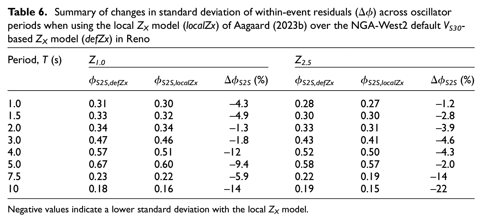
Negative values indicate a lower standard deviation with the local Z_X model.

Figure 14.

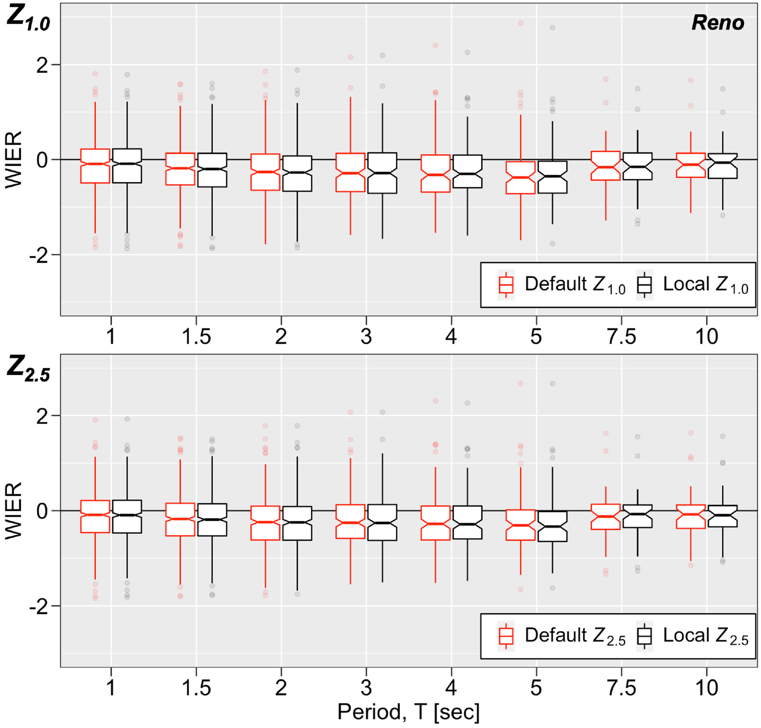
Boxplots showing change in mean values and standard deviations of within-event residuals (WIER) across oscillator periods when using the local Z_X model of Aagaard (2023b) over the NGA-West2 default V_S30-based Z_X model in Reno, Nevada; top: Z_1.0, bottom: Z_2.5. The box delineates the 25th, 50th (median), and 75th percentiles; the vertical lines (whiskers) extend either direction to 1.5 times the inter-quartile range (IQR, the difference between the value and the 75th and 25th percentiles); and the outliers beyond the whiskers are represented with circular symbols. Notches in the boxplot span the value of 1.58 times the IQR divided by the square root of the number of points, providing roughly a 95% confidence interval for comparing medians. Supplemental Tables S5 to S8 give the corresponding medians and standard deviations.

Portland, Oregon

The geological complexity of the Portland region stems from active subduction-zone tectonics and tertiary-age lava flows that challenge the classic definition of a sedimentary basin, especially as modeled using California-centric GMMs, where the gradient in V_S tends to increase monotonically with depth. The prominent Columbia River Basalt Group creates topographic highs of relatively competent material (basalt and weathered basalt), coincident with the northwest-striking Portland Hills fault. The relatively shallow Portland basin, situated north and east of the Portland Hills fault, exhibits a maximum Z_1.0 of about 0.55 km in the NCM (Aagaard, 2023a); the maximum value at a seismic station is 0.38 km. Z_2.5 in the Portland basin is also relatively shallow, averaging around 0.70 km for sites having Z_1.0 > 0.50 km (maximum 1.0 km), indicating the presence of a relatively large impedance contrast over a small depth range at the base of tertiary sediments. The Columbia River Basalt Group also produces velocity inversions at depth, where it overlies tertiary sediments in the deeper Tualatin basin structure, located southwest of the Portland Hills fault (Scanlon et al., 2021). In contrast with the Portland basin, Z_2.5 is as deep as 5.6 km in the Tualatin basin.

No stations in our data set are situated in the deepest parts of the Portland basin (Z_1.0 > 0.50 km); only 15 stations, comprising 81 ground-motion records, have Z_1.0 > 0.30 km, but all these stations also have δZ_1.0 < 0, indicating that the Z_1.0 values are shallower than average for the V_S30 at each station. In fact, 61 of the 71 stations in the Portland-region data set have δZ_1.0 < 0, predicting deamplification relative to the default V_S30-based site term in BSSA14. Conversely, ten stations in the Tualatin sub-basin (comprising 47 ground-motion records) have Z_2.5 ≥ 3 km, which would predict amplification using the CB14 basin term. We discuss results of residuals analyses both in terms of the full data set and in terms of the subset of sites that would experience basin amplification based on the respective basin terms in each GMM.

Binned mean values of δW_T,def show weak correlation with δZ_1.0 (Figure 15) and Z_2.5 (Figure 16) for T ≥ 1.0 s. We observe positive (underprediction) bias in the residuals for T ≤ 2 s (Figure 17), coupled with reduction of ϕ _S2S across all periods in the standard deviation when using the local Z_1.0 model, with an improvement of 15%–27% for T ≥ 4 s (Table 7). However, unlike the Great Valley, we do not have a substantial reduction in the standard deviation across all stations when using the local Z_2.5 model over the default model (Figure 17 and Supplemental Tables S9 and S10). Instead, we have an increase in the standard deviation of up to 9% across nearly all periods of interest. The relation between δS2S_j and Z_X (Figures S11 and S12 in the electronic supplement) exhibit similar trends to the WIER in Figures 15 and 16, but similar to Reno, there are a relatively small number of stations, especially at longer periods.

Figure 15.

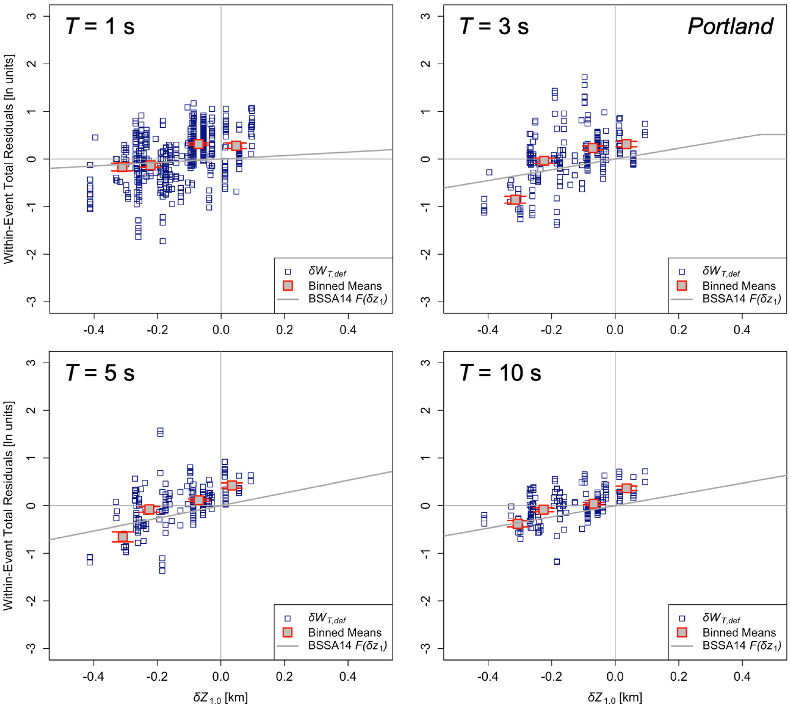
Empirical basin-depth scaling in Portland/Tualatin as compared to the Boore et al. (2014; BSSA14) ground-motion model as a function of δZ_1.0 for four periods of interest (T = 1.0, 3.0, 5.0, and 10 s). The rectangles denote the total within-event residuals for default V_S30-based Z_X values (δW_T,def) as well as the binned mean values and their standard deviations. The electronic supplement includes plots for ten oscillator periods between 0.5 and 10 s (Supplemental Figure S5).

Figure 16.

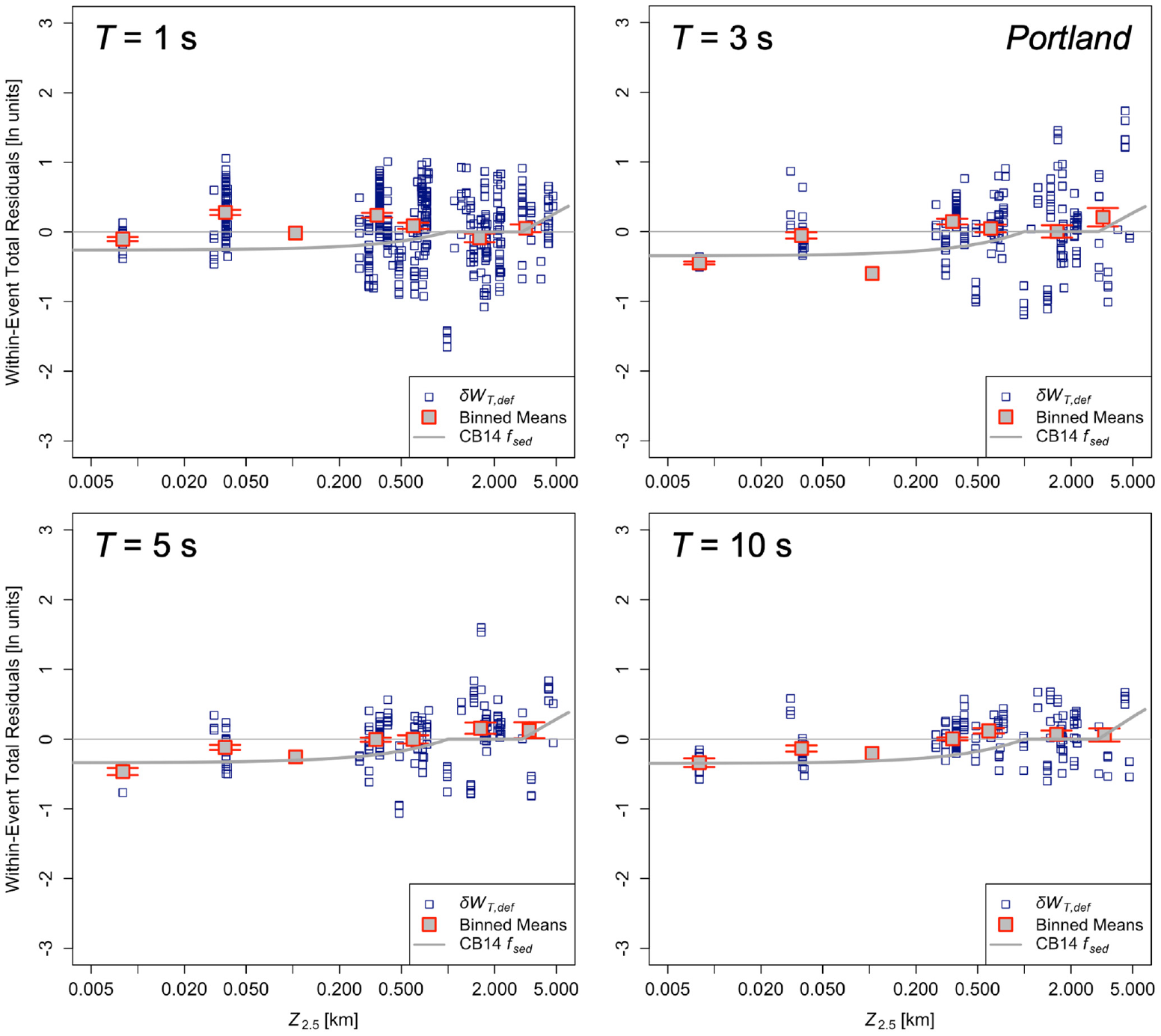
Empirical basin-depth scaling in Portland/Tualatin as compared to the Campbell and Bozorgnia (2014; CB14) ground-motion model as a function of Z_2.5 for four periods of interest (T = 1.0, 3.0, 5.0, and 10 s). The rectangles denote the total within-event residuals for default V_S30-based Z_X values (δW_T,def) as well as the binned mean values and their standard deviations. The electronic supplement includes plots for ten oscillator periods between 0.5 and 10 s (Supplemental Figure S6).

Figure 17.

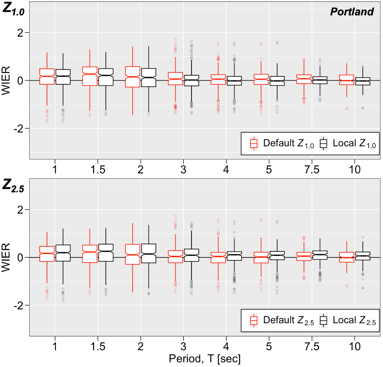
Boxplots showing change in mean values and standard deviations of within-event residuals (WIER) across oscillator periods when using the local Z_X model of Aagaard (2023a) over the NGA-West2 default V_S30-based Z_X model in Portland; top: Z_1.0, bottom: Z_2.5. The box delineates the 25th, 50th (median), and 75th percentiles; the vertical lines (whiskers) extend either direction to 1.5 times the inter-quartile range (IQR, the difference between the value and the 75th and 25th percentiles); and the outliers beyond the whiskers are represented with circular symbols. Notches in the boxplot span the value of 1.58 times the IQR divided by the square root of the number of points, providing roughly a 95% confidence interval for comparing medians. Supplemental Tables S9 to S12 give the corresponding medians and standard deviations.

Table 7.

Summary of changes in standard deviation of within-event residuals (Δϕ) for all sites across oscillator periods when using the local Z_X model (localZx) of Aagaard (2023a) over the NGA-West2 default V_S30-based Z_X model (defZx) in Portland

Period, T (s)	Z1.0			Z2.5
	ϕS2S,defZx	ϕS2S,localZx	ΔϕS2S (%)	ϕS2S,defZx	ϕS2S,localZx	ΔϕS2S (%)
1.0	0.43	0.42	−4.2	0.41	0.43	+4.3
1.5	0.46	0.43	−7.0	0.44	0.44	+0.7
2.0	0.50	0.47	−7.5	0.48	0.48	+1.0
3.0	0.54	0.48	−11	0.52	0.52	+0.8
4.0	0.47	0.40	−15	0.45	0.44	−0.7
5.0	0.45	0.38	−16	0.42	0.41	−3.3
7.5	0.33	0.24	−27	0.31	0.33	+7.2
10	0.30	0.24	−21	0.29	0.32	+9.0

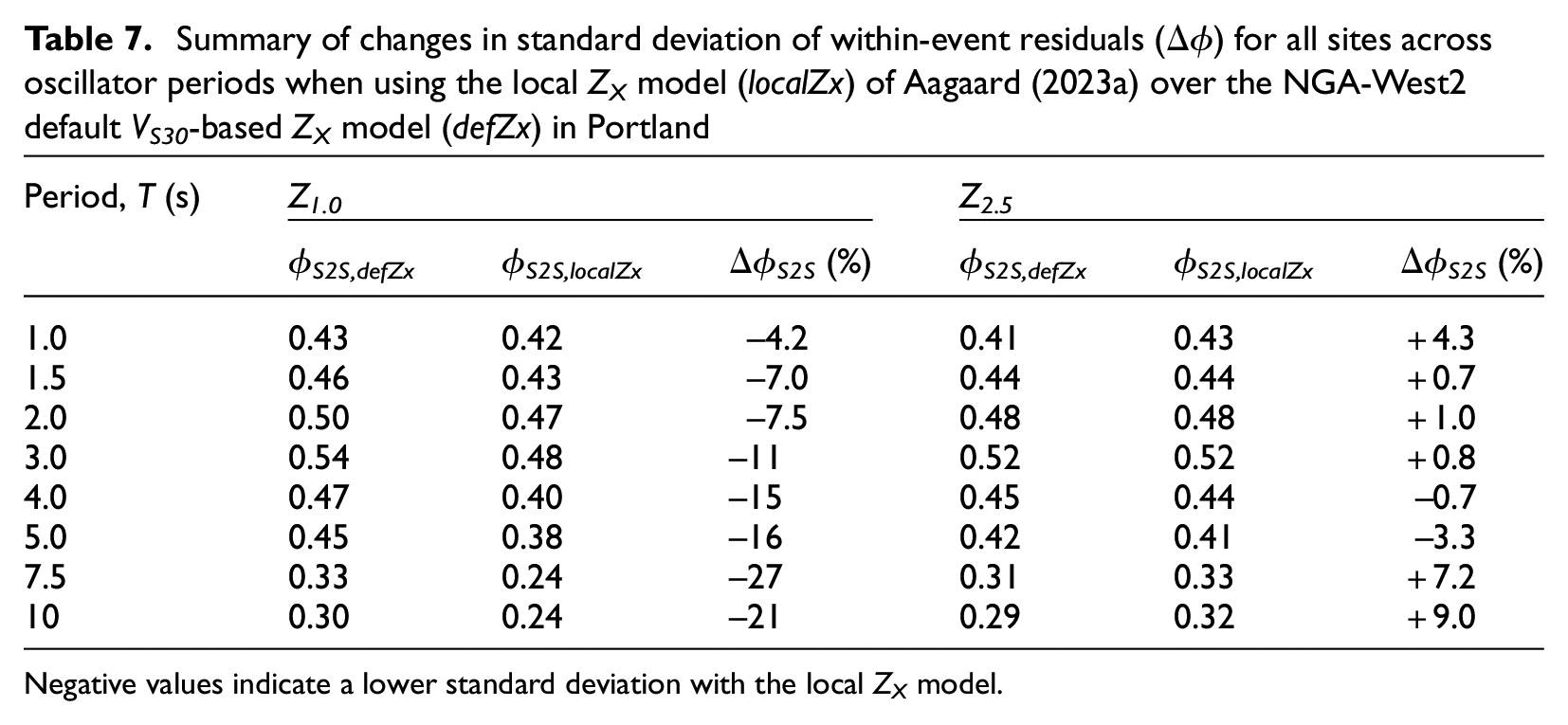
Negative values indicate a lower standard deviation with the local Z_X model.

We performed additional analysis for the subset of stations for which the GMMs predict basin amplification (δZ_1.0 > 0 for BSSA14; Z_2.5 > 3 km for CB14). Tables S9 to S12 in the electronic supplement show results for analysis of ϕ _S2S for these stations, including mean values and standard deviations of WIER (μ_WIER and ϕ, respectively) for Z_1.0 and Z_2.5. The percent reduction in ϕ _S2S with the local Z_2.5 increases substantially for periods greater than 1.5 s when we only consider stations where amplification is predicted; the mean bias in WIER decreases more than 50% at periods between 2.0 and 5.0 s for both local Z_1.0 and Z_2.5 basin-depth models. The bias does increase at these deep-basin sites for Z_2.5 at periods of 7.5 and 10 s. Thus, we find the local basin-depth models in Portland improve the accuracy of the GMMs as quantified by reductions in the mean bias and standard deviation of WIERs, although there are some exceptions. Variations in the improvement or lack thereof in these metrics likely arise from the complex 3D structure that includes tertiary-age lava flows and deep tertiary sediments in the Tualatin basin.

Discussion

Our analysis of ground-motion records in the California Great Valley demonstrates that the NGA-West2 GMMs are consistent with the observed basin amplification. This basin also meets the minimum depth constraints (Z_2.5 > 3 km, corresponding to ground-motion amplification) imposed in the 2018 NSHM update. Including local basin depths in the NSHM for the Great Valley using the local Z_X models would greatly expand the fraction of California covered by local basin models. Furthermore, the consistency of the observed basin response in the Great Valley with the GMM predictions indicates that future updates of the NSHM could consider expanding the regions in California covered by local basin-depth models, assuming appropriate Z_X models exist. For example, the western portion of California along the San Andreas fault system may exhibit behavior similar to the Los Angeles and San Francisco Bay regions used to develop the basin terms in the GMMs and the Great Valley. On the contrary, ground motions in other regions, especially those with extensive shallow volcanic geologic units, may exhibit different behavior. To expand the use of sedimentary basin terms in the GMMs in California, we need validated models for both Z_1.0 and Z_2.5. We usually extract Z_X from 3D seismic velocity models, but many lack sufficient resolution at shallow depths (e.g., Shaw et al., 2015) to provide reasonable estimates of Z_1.0 except in limited areas. Seismic velocity models that incorporate a wide variety of constraints, as in the USGS San Francisco Bay regional 3D seismic velocity model (Aagaard and Hirakawa, 2021) and the USGS NCM (Boyd and Shah, 2018), tend to provide more accurate Z_X values over broad regions than seismic velocity models based on seismic tomography.

Our epistemic uncertainty analysis for the basin terms in BSSA14 and CB14 resulting from uncertainty in the basin depth of the Great Valley yields uncertainties in spectral acceleration of 0.06–0.08 ln units for 3.0 ≤ T ≤ 10 s. Because the basin term in BSSA14 depends on relative, rather than absolute, basin depth, the uncertainty in the basin term is independent of absolute basin depth even though uncertainty in geologic structure usually increases with depth. However, the basin term exhibits a strong dependence on period, which results in the uncertainty in the basin term also having a strong dependence on period. In contrast, the uncertainty in the basin term in CB14 exhibits little sensitivity to period, but the uncertainty does depend on absolute basin depth. The exponential form of the basin-depth term in CB14 leads to decreasing uncertainty in the basin term as the basin depth increases. For example, an uncertainty of 500 m in Z_2.5 results in relatively small uncertainties in spectral acceleration at T = 5.0 s of 0.07 and 0.03 ln units (3%–7%) for basin depths of 4 and 8 km, respectively. The discrepancies between BSSA14 and CB14 in the dependence of uncertainty in the basin terms on period and basin depth indicate additional work could refine the functional form of the basin-depth terms to accurately capture both the basin response and its epistemic uncertainty.

The Reno basin is substantially shallower than the Great Valley even though V_S30 values are similar. Consequently, at most sites, the basin terms in BSSA14 and CB14 predict deamplification. We do not find significant correlation of basin response with δZ_1.0 and Z_2.5 for Reno. The improvement of GMM performance, as measured by the reduction in the standard deviation of the site-to-site residuals ϕ _S2S when using the local Z_X models, is much smaller than what we observe for the Great Valley with values at most periods less than 5%. Although the reductions at a period of 10 s are relatively larger, only a few ground-motion records and stations contribute to these observations, so we have much less confidence in the improvement. In addition, we find substantial overprediction in the ground motions across all periods for both the default V_S30-based basin depths and the local basin depths.

We did not consider the local Z_X models from the NCM for Reno. Nevertheless, the NCM yields Z_X models quite similar to those from Simpson and Louie (2020). The consistency of these Z_X models gives us confidence in the basin-depth models, which indicates that the Reno basin exhibits substantially different behavior than the basins in California used to guide the development of the basin amplification terms in BSSA14 and CB14. Thus, we believe BSSA14 and CB14 do not accurately capture the site and basin response in Reno. Additional work could improve the site and basin response models in these GMMs for shallow basin structures like those in Reno.

The Portland and Tualatin basins in Oregon are geologically more complex than the California Great Valley and those in Reno, Nevada, which is evident in the basin response. Using the local Z_1.0 model with the Portland data set provides the best improvement of ground-motion prediction of any of our three study regions as measured by the reduction in ϕ _S2S ; conversely, use of the candidate Z_2.5 model across the Portland region did not improve GMM predictions from the perspective of a reduction of ϕ _S2S . However, we do find the mean bias of the WIERs decreases by 50% or more across a wide range of periods (1.0 s ≤ T ≤ 5.0 s) with the use of the local basin-depth models for both BSSA14 and CB14. If we limit our assessment to just stations where the GMMs predict amplification, then the predictions with respect to ϕ _S2S improve across almost all periods between 3.0 and 10 s with the use of the local basin-depth models.

Frankel and Grant (2020) observed basin amplification of a factor of 10 at periods of 2.0–3.0 s at station SAIL (45.5371°N, 122.9628°W, V_S30 = 301 m/s; Z_1.0 = 360 m), relative to a single rock site. Because they compute amplification relative to a rock site, the amplification includes contributions from both shallow and deep structure. In our analysis, which includes 15 ground-motion records at station SAIL, we also observe amplification (refer to Figure 16, T = 3.0 s, furthest upper-right data points), with WIERs ranging from 1.21 to 1.73 ln units (or an amplification factor of 3.4–5.6). Because we remove the site term from the WIER, which includes both shallow and some deep basin response, we compute less amplification than that computed by Frankel and Grant (2020). Nevertheless, at most periods greater than 2.0 s, we do find the local basin-depth models improve the ground-motion predictions as measured by a reduction in the mean bias and ϕ _S2S for stations where amplification is predicted.

Collecting additional data and assessing site and basin amplification for each of the Portland and Tualatin basins will help further characterize the response of these complex geologic structures. Assessing basin response using NGA-Subduction GMMs and related site response models (e.g., Parker and Stewart, 2022), which were created solely with subduction-zone data and regionalized for Cascadia, could also further constrain basin response in the Portland basin, as has been done in the Seattle basin for the 2023 NSHM update (Moschetti et al., 2024).

In all three regions, better site and basin characterization would improve (1) prediction of V_S30-based site-amplification terms, (2) prediction of Z_1.0 and Z_2.5, which would likely lead to better performance of GMMs based on Z_X, and (3) characterization of the site and basin response and allow more sophisticated models of site and basin response in GMMs. For example, GMMs with spatially variable coefficients could also explicitly incorporate local adjustments to site and basin response.

Conclusion

The NGA-West2 GMMs used in the NSHM perform well with our local basin-depth models for the California Great Valley. Our analysis provides additional evidence that basins in California besides those used to develop the GMMs may display behavior consistent with current GMMs, and future updates to the NSHM might be able to use local Z_X models over a much larger portion of California. The GMMs do not perform as well for the relatively shallow and small basins underlying Reno, Nevada, which exhibit much less sensitivity to the predictor variables used in the NGA-West2 GMMs. The basin response is more complex in the Portland, Oregon region; the local Z_1.0 model yields substantial reductions in the uncertainty in the ground-motion predictions, whereas the local Z_2.5 model consistently improves ground-motion predictions only in the deepest part of the Tualatin basin.

No ergodic, global, 1D GMM will capture complex phenomena of site and basin response in 3D geologic basins. Nonergodic GMMs developed from local data will almost certainly yield more accurate predictions of ground motion (Lavrentiadis et al., 2022). However, such models require large empirical or synthetic data sets and are relatively early in their evolution. Expanding the regions using local basin-amplification models and using simulations to derive local basin-amplification factors are important steps toward including nonergodic GMMs in future updates of the NSHM.

Supplemental Material

sj-docx-1-eqs-10.1177_87552930241237250 – Supplemental material for Empirical ground-motion basin response in the California Great Valley, Reno, Nevada, and Portland, Oregon

Supplemental material, sj-docx-1-eqs-10.1177_87552930241237250 for Empirical ground-motion basin response in the California Great Valley, Reno, Nevada, and Portland, Oregon by Sean K Ahdi, Brad T Aagaard, Morgan P Moschetti, Grace A Parker, Oliver S Boyd and William J Stephenson in Earthquake Spectra