Sage Journals: Discover world-class research

Abstract

In recent decades, probabilistic earthquake risk estimation has evolved significantly, with the FEMA P-58 methodology emerging as the method of choice for practical seismic risk assessments of buildings. Few studies, however, have examined the level of contribution of the explicitly modeled sources of uncertainty to the estimated losses. This study quantifies those contributions for intensity-based assessments utilizing variance-based sensitivity analysis (VBSA) and examines how they are affected by a variety of parameters. Considered sources of uncertainty include the variability of engineering demand parameters (EDPs) for a given level of shaking, the uncertain component quantities, the uncertain capacities defined by the fragility curves, and the uncertainty in the damage consequences. Their contributions are examined through the lens of factor prioritization. Our findings highlight the significant role of the building replacement likelihood in altering the variance contributions, with a predominant contribution of its associated sources of uncertainty at high levels of shaking. They also reveal a consistently high contribution of peak floor accelerations (PFAs) and residual interstory drifts (RIDs) compared with other EDPs and demonstrate the implications of crudely defined component damage models. By revealing the contribution breakdown for a variety of cases, the study enables a more effective allocation of resources and offers a broader intuition on the inner workings of loss estimation.

Keywords

earthquake risk estimation performance-based engineering FEMA P-58 variance-based sensitivity analysis uncertainty

Introduction

In recent years, earthquake risk estimation has seen wide adoption, enabling engineers to quantify the likelihood of potential impacts on assets. One of the most prominent earthquake risk estimation methodologies is outlined in the FEMA P-58 series of reports. The FEMA P-58 methodology utilizes a damage and loss estimation process involving uncertainty quantification to produce probability distributions of performance measures. These distributions can then be utilized to support evidence-based decision-making. By enabling the prediction of easily interpretable performance measures, the framework contributes to the ongoing shift of societal expectations toward more resilient infrastructure and faster disaster recovery (Sattar 2021).

Recognizing the inherent uncertainty associated with certain variables, the FEMA P-58 methodology treats them as random and utilizes Monte Carlo simulation (MCS) to propagate their variance to the estimated loss measures. In the context of this study, we will use the term uncertain factors to refer to these random variables. Despite the growing use of performance-based earthquake engineering (PBEE)—in applications such as optimized design (Steneker et al. 2020), community resilience assessment (Cook et al. 2022), or resilience-focused engineering optimization (Issa et al. 2023)—few studies have focused on how uncertainty propagates from these uncertain factors to the loss measures. Excessive variance in the estimated loss measures is undesirable as it can impact the credibility of the analysis results. It can also introduce bias in the loss estimates due to the complicated nature of uncertainty propagation. When examining whether uncertainty can be reduced, it is useful to know what uncertain factors contribute the most, as reducing uncertainty in those sources would have the greatest impact on lowering the output variance. In the context of sensitivity analysis, this goal is referred to as factor prioritization (Saltelli et al. 2008) and is a primary objective of this study.

In related research, Bradley (2013) highlighted certain misconceptions regarding uncertainty in PBEE computations, pointing out that lack of hazard consistency in ground motion selection amplifies the uncertainty that is perceived to be coming from the seismic hazard. Bradley called for a reconsideration of the typically assumed modeling uncertainty. Iervolino (2017) provided ways of examining the effects of uncertainty attributed to ground motion record-to-record variability on the derivation of structural fragility curves. While these studies focus on uncertainty quantification, they provide insight limited to structural performance metrics.

Uncertainty propagation has been studied extensively in the context of probabilistic seismic hazard analysis (PSHA), a crucial step in PBEE. Field et al. (2020) ranked various sources of epistemic uncertainty inherent in PSHA computations based on their contribution to the variance of the estimated average annual loss (AAL) for California, aiming to guide research efforts. Another building portfolio-level study quantifying the effects of uncertainty was conducted by Aslani et al. (2012), finding that seismic hazard uncertainty contributed significantly to the overall loss uncertainty, followed by uncertainties in building vulnerability.

A limited number of studies have applied variance-based sensitivity analysis (VBSA) on damage and loss frameworks to rank the relative contributions of uncertain factors. Rohmer et al. (2014) used VBSA to compare the relative contribution of several model parameters associated with earthquake-induced damage estimation relying on the European Macroseismic Scale damage grades. They found that uncertainty associated with the seismic hazard had the highest contribution to the uncertainty of the loss assessment results, followed by the uncertainty coming from the damage and loss steps. While none of the above studies considered the uncertainty in fragility and damage consequences of individual structural or nonstructural building components, Cremen and Baker (2021) used VBSA to rank the relative contribution of input uncertainty to losses estimated with FEMA P-58, revealing that shaking intensity and building age were the most significant contributors to the repair cost uncertainty. To the authors’ knowledge, this was the first study to apply VBSA to FEMA P-58 loss estimation results. The study examined how much uncertainty in higher-level input parameters (i.e., those affecting the evaluation inputs, such as the building’s age and structural system) contributes to the loss variance of individual assessments, assuming that such parameters are the dominant source of uncertainty. However, in many performance evaluation applications, such higher-level input parameters are known with certainty. When that is the case, there has not been a comprehensive examination of the contribution of sources of uncertainty that are inherent to the methodology and necessarily propagated during its application, such as the uncertainty in the damage capacity and repair cost of building contents or the collapse capacity and replacement cost of the building.

We have initiated a research endeavor to better understand the uncertainty contribution of all random variables involved in FEMA P-58 intensity-based assessments (Vouvakis Manousakis and Konstantinidis 2022). Our preliminary findings on repair cost suggested that the predominant uncertain factors in FEMA P-58 loss estimates for a given intensity measure are the building’s response and the uncertainty in the component and building fragility curves. Our study highlighted the increase in relevance of the component fragility uncertainty when the performance model includes high-dispersion judgment-based fragility curves and demonstrated how VBSA can be applied to reveal the extent of contribution of any uncertainty source that is directly considered when generating loss realizations. This prior work set the foundation for our current study, offering an initial understanding of how the relative contributions change as the intensity measure increases and the implications of using a performance model with a lower fidelity level. Recently, a study by Kourehpaz et al. (2023) has also contributed to this research area. Examining a reinforced concrete shear wall building, the authors studied the contribution of a set of uncertain factors to the probability of irreparable damage and the estimated repair cost. Their work offers an additional demonstration of the applicability of VBSA to identify the relative contribution of uncertain factors. It confirms the shifting nature of their variance contribution at different intensity levels.

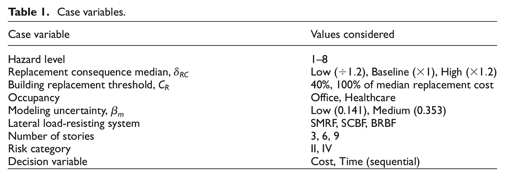
In light of these developments, the present study aims to build on our preliminary findings. We consider a broader range of performance evaluation scenarios to demonstrate the influence of a variety of case variables on the relative contribution of uncertain factors to the loss variance for intensity-based assessments (i.e., conditioned on a particular intensity measure). The case variables we examine are summarized in Table 1. We partition all uncertain factors involved in damage and loss estimation into groups based on their function in the overall performance evaluation framework and examine the relative contribution of the groups for all case variable combinations under the lens of factor prioritization. The uncertain factor groups are shown in Table 2.

Table 1.

Case variables.

Case variable	Values considered
Hazard level	1–8
Replacement consequence median, $δ_{RC}$	Low ( $\div 1.2$ ), Baseline ( $\times 1$ ), High ( $\times 1.2$ )
Building replacement threshold, $C_{R}$	40%, 100% of median replacement cost
Occupancy	Office, Healthcare
Modeling uncertainty, $β_{m}$	Low (0.141), Medium (0.353)
Lateral load-resisting system	SMRF, SCBF, BRBF
Number of stories	3, 6, 9
Risk category	II, IV
Decision variable	Cost, Time (sequential)

Table 2.

Uncertain factor groups.

Tag	Contained uncertain factors
EDP	Building response variables (PID, RID, PFA, PFV) conditioned on an IM.
C-Q	Component quantities.^a
C-DM	Component fragility capacity and realized consequence.^b
C-DV	Component unit loss measures conditioned on a realized consequence.^c
B-DM	Building collapse and excessive residual drift fragility capacity.
B-DV	Building replacement loss measures.^c

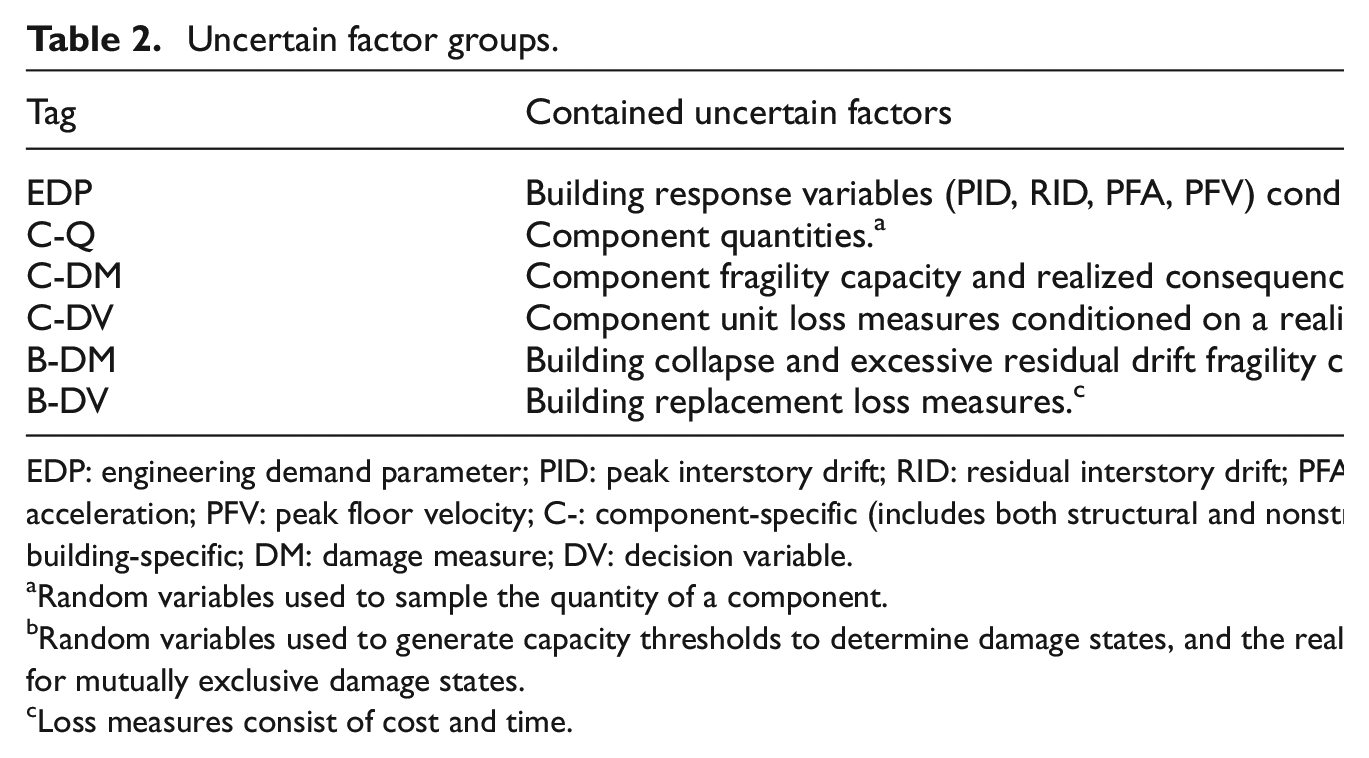
EDP: engineering demand parameter; PID: peak interstory drift; RID: residual interstory drift; PFA: peak floor acceleration; PFV: peak floor velocity; C-: component-specific (includes both structural and nonstructural); B-: building-specific; DM: damage measure; DV: decision variable.

Random variables used to sample the quantity of a component.

Random variables used to generate capacity thresholds to determine damage states, and the realized consequences for mutually exclusive damage states.

Loss measures consist of cost and time.

Our study aims to yield more generalized insights, offering analysts a deeper understanding of how uncertain factors affect the results for any given set of case variables and further exemplify the applicability of VBSA to quantify their contribution in any application of the FEMA P-58 methodology. Unlike Kourehpaz et al. (2023), who assume randomness in the distribution parameters of random variables, we focus on the outcomes of “standard” intensity-based FEMA P-58 evaluations without this assumption. In addition, instead of only considering excessive drift, we include factors such as collapse and excessive cost in our building replacement probability calculations. A key objective of our study is to enable the prioritization of uncertainty reduction efforts under the setting of an intensity-based evaluation of a given asset. Our inputs are based on the assumption that effort has already been made to reduce uncertainty where possible, leading to the utilization of a high-fidelity structural model and relatively small component quantity uncertainty.

Summary of the Theoretical Framework

Variance-Based Sensitivity Analysis

With the objective of breaking down the contributions of individual uncertain factor groups to the loss variance, this section presents a brief overview of VBSA.

A stochastic model

Y = f (X_{1}, X_{2}, \dots, X_{m})

(1)

utilizes random variables, $X_{i}$ , to simulate the uncertainty associated with what they represent. The uncertainty is propagated to the final result, $Y$ , which is, therefore, a random variable as well. The model can also include deterministic parameters. The terms inputs and output are typically used to refer to the random variables, $X_{i}$ , and the result, $Y$ . Variance-based sensitivity analysis (VBSA), as the name implies, aims to quantify the sensitivity of the variance of an output variable to the variance of the inputs (Saltelli et al. 2008). The method relies on the law of total variance:

V [Y] = \underset{(A)}{\underset{︸}{E_{X_{i}} [V_{X_{- i}} [Y | X_{i}]]}} + \underset{(B)}{\underset{︸}{V_{X_{i}} [E_{X_{- i}} [Y | X_{i}]]}}

(2)

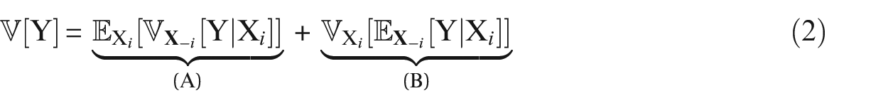
Term (A) in this equation represents the expected variance of the output when the input in question, $X_{i}$ , is fixed to some value, where $E_{X_{i}}$ denotes the expectation taken under the distribution of $X_{i}$ , and $V_{X_{- i}}$ denotes the variance taken under the distribution of all other inputs except $X_{i}$ . When conditioning results in a large reduction in the output variance, this suggests that the considered input is an important contributor. To quantify the relevance of that input, term (B) of Equation 2 is normalized against the original output variance to yield a sensitivity index, $s_{i}$ , that is proportional to the relative contribution of input $X_{i}$ :

s_{i} = \frac{V_{X_{i}} [E_{X_{- i}} [Y | X_{i}]]}{V [Y]}

(3)

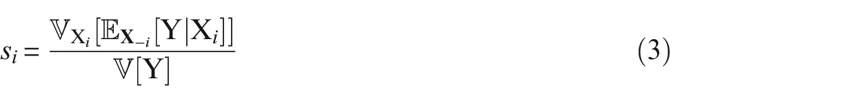
Input variables can affect the output variance individually and through interactions with other input variables. We refer to these effects as primary and higher-order, respectively. Such higher-order effects can be captured by partitioning the input variables in groups and considering their collective contribution:

s_{g} = \frac{V_{X_{g}} [E_{X_{- g}} [Y | X_{g}]]}{V [Y]}

(4)

where $E_{X_{- g}}$ denotes the expectation taken under the joint distribution of all random variables except those in the considered group, $X_{- g}$ , and $V_{X_{g}}$ denotes the variance taken under the joint distribution of the considered group of random variables, $X_{g}$ . Equation 4 quantifies the collective primary effect of all random variables in the considered group and all higher-level interactions between random variables within that group. To simplify the terminology, in this paper, we will refer to $s_{g}$ as the primary effect sensitivity index of group $g$ , even though it includes the interactions of the individual random variables that belong in it. It is easy to see that Equation 3 is a special case of Equation 4, where the considered group only contains a single random variable.

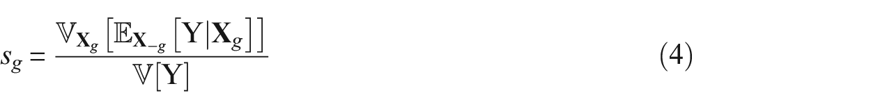
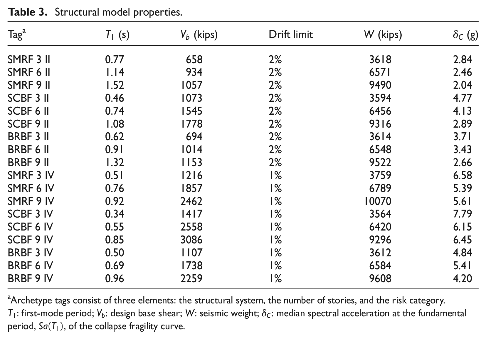
To get a complete picture of the effect of a group on the output variance, it is also important to include higher-order interactions of the inputs within the group and the rest of the inputs of the model. Such interactions are captured by the total-effect sensitivity index of a given group, which includes the primary effects, all higher-order interactions within the group, as well as all higher-order interactions between inputs that belong to the group and inputs outside of it:

s_{T, g} = \frac{E_{X_{- g}} [V_{X_{g}} [Y | X_{- g}]]}{V [Y]}

(5)

This sensitivity index only excludes the primary effect and higher-order interactions that do not involve any of the inputs in the considered group.

Whether it refers to a single input or a group, a primary effect sensitivity index close to one indicates a substantial contribution to the output variance. However, even when the primary effect is small, interactions can be significant enough that the considered input or group remains a relevant contributor. Therefore, a small primary effect does not necessarily imply that the input or group in question has a small contribution unless the total-effect sensitivity index is also small. A total-effect sensitivity index close to zero suggests that the variance of the corresponding input has minimal contribution to the output variance and can be fixed to its expected value without affecting the results.

Since the total variance of the output is the result of first-order effects and higher-order interactions between the random inputs, when interactions are present, the sum of the first-order sensitivity indices of all groups does not reach the value of one, even when the groups cover an exhaustive set of all associated random variables. Similarly, the sum of all total-effect group sensitivity indices exceeds the value of one in those cases since multiple groups capture interactions between the same random variables.

In most cases, the complexity of the considered stochastic model prohibits the direct use of the definitions in Equations 3 to 5. While it is possible to estimate the individual components with MCS, researchers have proposed estimators that require far fewer realizations to arrive at a robust estimate and yield both the first-order and the total-effect sensitivity indices (Saltelli et al. 2010).

FEMA P-58 Damage and Loss Calculations

The damage and loss estimation process of the FEMA P-58 methodology propagates the uncertainty of various inputs to quantify the probability of exceedance of loss measures conditioned on the occurrence of an IM, and is therefore a stochastic model. The methodology is outlined in detail in the first volume of FEMA P-58 (FEMA 2018a). Here we offer a brief overview for the benefit of the reader.

In the case of an assessment involving detailed structural analysis, a conditioning value of a chosen IM is used to construct a target spectrum and select a suite of representative ground motions. A structural model is analyzed to obtain the building response for each ground motion, resulting in a set of engineering demand parameters (EDPs) relating to the IM corresponding to the suite. The results are used to fit a probability distribution, allowing for the generation of an arbitrarily large set of building response realizations conditioned on the IM. Consequently, simulated EDPs are treated as a random vector, the joint distribution of which is one of the inputs of the stochastic model.

The following steps involve estimating damage and losses. A performance model defines the building components capable of producing losses under earthquake shaking. The quantities of the components can be fixed or defined with probability distributions, which can be viewed as additional uncertain inputs of the stochastic model. The EDPs associated with each component are compared with their capacity defined by one or more fragility curves, resulting in their realized damage states. Each damage state can be associated with one or more consequences. For any given consequence, the realized loss is determined by utilizing a random variable that defines the unit loss measure, which is then used in tandem with the realized component quantities to obtain the losses, adjusting for economies of scale. Therefore, determining the capacity and realized consequence involves using random variables that can be treated as inputs to the stochastic model, similar to the EDPs or the component quantities.

The methodology distinguishes cases where the building is damaged beyond repair, where the losses are driven by building replacement, while individual component-driven losses are ignored. Building replacement is triggered by three events: collapse, excessive residual drift, or excessive realized repair costs. A collapse fragility curve is used to determine instances of building collapse, introducing a random variable representing the building’s capacity. Residual drift is estimated from the peak story drift realizations, and a fragility curve represents the residual drift capacity. Instances of exceedingly large repair cost are identified by comparing the realized losses driven by individual components with a limit value. The limit value is the expected building replacement cost, adjusted to account for the fact that building owners tend to replace a heavily damaged building even when the repair cost is smaller than the replacement cost.

It becomes clear that the damage and loss estimation process involves a large number of random variables affected by the size of the building and the performance model. Regardless of their number, it is possible to arrange them into groups based on what they represent. This study uses the grouping scheme defined in Table 2.

Definition of Performance Evaluation Scenarios

Site Details, Archetype Buildings, and Seismic Hazard

All of the structural archetypes we examine are assumed to be located at a site in Berkeley, CA (–122.259, 37.871) to obtain results representative of a high seismic area. To quantify the seismic hazard for the site, we used OpenSHA, version 1.5.2 (Field et al. 2003). According to the CGS/Wills Vs30 Map, the site has a Vs30 of 260 m/s (Wills et al. 2015).

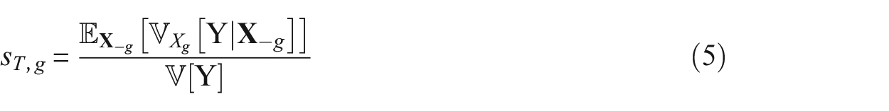
The analyzed set of archetype buildings includes three structural system configurations, with three, six, or nine stories, and two risk category (RC) variations, RC II and IV, as defined in ASCE 7-22. The three structural systems are special moment-resisting frames (SMRFs), special concentrically braced frames (SCBFs), and buckling-restrained braced frames (BRBFs), aiming to cover a variety of potential structural responses for a given level of shaking. As shown in Figure 1, all archetypes share the same plan layout dimensions, with differences in the placement of the lateral load-resisting members.

Figure 1.

Plan layout of all archetypes. (a) Moment frame archetypes. (b) Braced frame archetypes.

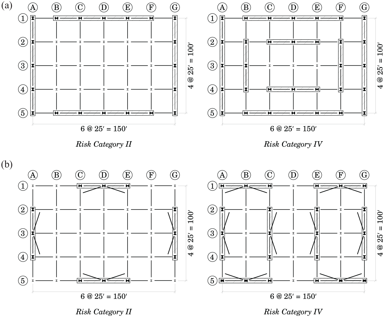
For any given archetype, the lateral load-resisting members are identical in both primary horizontal directions. All stories have a height of 13 feet except the first, which has a height of 15 feet. The archetypes were designed for the seismicity of the site employing modal response spectrum analysis in accordance with ASCE 7-22 and the referenced provisions for the design of steel buildings (AISC 341-16; AISC 360-16; AISC 358-16). As seen in Figure 1, RC II archetypes feature lines of lateral load-resisting elements only in their perimeter, while RC IV archetypes include additional internal lines of resistance. For moment frames, beam/column joints were designed assuming a welded, unreinforced flange-welded web connection. Beams and columns have W-section shapes with an ASTM material specification of A992 and a nominal yield stress of 50 ksi. Braced frames feature single-bay braces in a two-story X configuration. SCBF braces have circular HSS sections with A500 grade B steel, having a nominal yield stress of 42 ksi. Their gusset plates were designed following the elliptical clearance method proposed by Roeder et al. (2011). BRBF braces were chosen by interpolating the options listed on the CoreBrace bolted brace design guide, assuming A36 steel with a nominal yield stress of 38 ksi and they feature more compact gusset plates (CoreBrace 2020). The first-mode period, design base shear, design drift limit, and seismic weight of the archetypes considered in this study are shown in Table 3. For brevity, elevation drawings showing the chosen member sections for each archetype are provided as supplemental material.

Table 3.

Structural model properties.

Tag^a	$T_{1}$ (s)	$V_{b}$ (kips)	Drift limit	$W$ (kips)	$δ_{C}$ (g)
SMRF 3 II	0.77	658	2%	3618	2.84
SMRF 6 II	1.14	934	2%	6571	2.46
SMRF 9 II	1.52	1057	2%	9490	2.04
SCBF 3 II	0.46	1073	2%	3594	4.77
SCBF 6 II	0.74	1545	2%	6456	4.13
SCBF 9 II	1.08	1778	2%	9316	2.89
BRBF 3 II	0.62	694	2%	3614	3.71
BRBF 6 II	0.91	1014	2%	6548	3.43
BRBF 9 II	1.32	1153	2%	9522	2.66
SMRF 3 IV	0.51	1216	1%	3759	6.58
SMRF 6 IV	0.76	1857	1%	6789	5.39
SMRF 9 IV	0.92	2462	1%	10070	5.61
SCBF 3 IV	0.34	1417	1%	3564	7.79
SCBF 6 IV	0.55	2558	1%	6420	6.15
SCBF 9 IV	0.85	3086	1%	9296	6.45
BRBF 3 IV	0.50	1107	1%	3612	4.84
BRBF 6 IV	0.69	1738	1%	6584	5.41
BRBF 9 IV	0.96	2259	1%	9608	4.20

Archetype tags consist of three elements: the structural system, the number of stories, and the risk category.

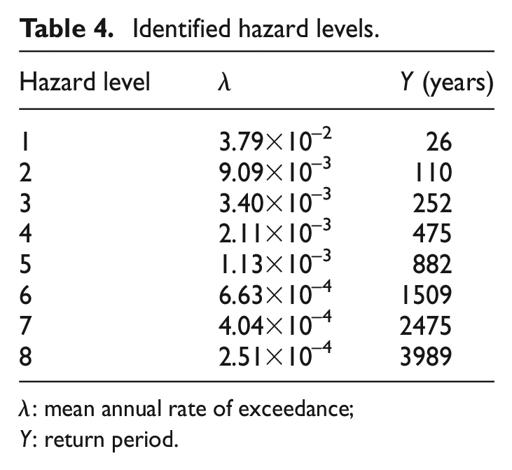
$T_{1}$ : first-mode period; $V_{b}$ : design base shear; $W$ : seismic weight; $δ_{C}$ : median spectral acceleration at the fundamental period, $Sa (T_{1})$ , of the collapse fragility curve.

Using OpenSHA, we utilized the mean UCERF3 earthquake rupture forecast (Field et al. 2014), assuming a Poisson model for the probability of earthquake occurrences, and the averaged 2014 NGA West ground motion models (Bozorgnia et al. 2014) to obtain a hazard curve for each archetype’s first-mode period and develop a uniform hazard spectrum (UHS) for a predefined set of return periods. These return periods define eight distinct hazard levels covering a broad range of shaking intensity intended to capture behavior ranging from minor to heavy damage. The mean annual exceedance rate and corresponding return period of the chosen hazard levels are shown in Table 4.

Table 4.

Identified hazard levels.

Hazard level	$λ$	$Y$ (years)
1	3.79×10^–2	26
2	9.09×10^–3	110
3	3.40×10^–3	252
4	2.11×10^–3	475
5	1.13×10^–3	882
6	6.63×10^–4	1509
7	4.04×10^–4	2475
8	2.51×10^–4	3989

$λ$ : mean annual rate of exceedance;

$Y$ : return period.

For each hazard level and using each archetype’s first-mode period, we constructed a conditional spectrum (CS), as outlined by Baker and Lee (2018), and selected a suite of 40 representative ground motions by matching the median rotated component (RotD50) of the two horizontal directions. Representing all target spectra led to a requirement of 722 unique ground motion records, most of which appear in multiple suites with differing scale factors with a maximum value of 4.7. The ground motions were retrieved from the PEER NGA-West 2 database (Bozorgnia et al. 2014). Constructing each CS required seismic hazard deaggregation data obtained using OpenSHA. While FEMA P-58 suggests the use of either UHS or conditional mean spectra (CMS) for time-based assessments, recent research has shown that ground motion selection using CS targets, which also account for ground motion model dispersion, results in a more consistent link between seismic hazard and structural response (Baker et al. 2014). Figure 2 illustrates a set of representative site-specific hazard curves and offers an example of target spectra and the corresponding ground motion suites associated with hazard levels 1, 2, 4, and 8 for the SMRF 3 II archetype. 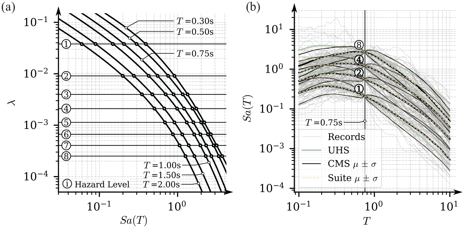In that figure, $μ$ represents the mean and $σ$ the standard deviation of the target spectra and ground motion suites.

Figure 2.

Representative hazard curves (a) and example of ground motion suites (b) (hazard levels 1, 2, 4, and 8, corresponding to the SMRF 3 II archetype).

For brevity, the list of the selected ground motions and their corresponding scale factors in each ground motion suite is reserved for the data repository that accompanies this study.

Structural Model Description

We developed a detailed nonlinear structural model of each archetype using OpenSees version 3.5.0, utilizing the Python interpreter (McKenna et al. 2010). The model definition was facilitated by osmg, a dedicated Python package developed for this purpose (Vouvakis Manousakis and Perez 2024). The developed models are three-dimensional, providing a detailed representation of the gravity framing members and enhancing the overall versatility of the models in terms of their potential use in future studies. Perspective views of the RC IV models, produced using osmg, are shown in Figure 3.

Figure 3.

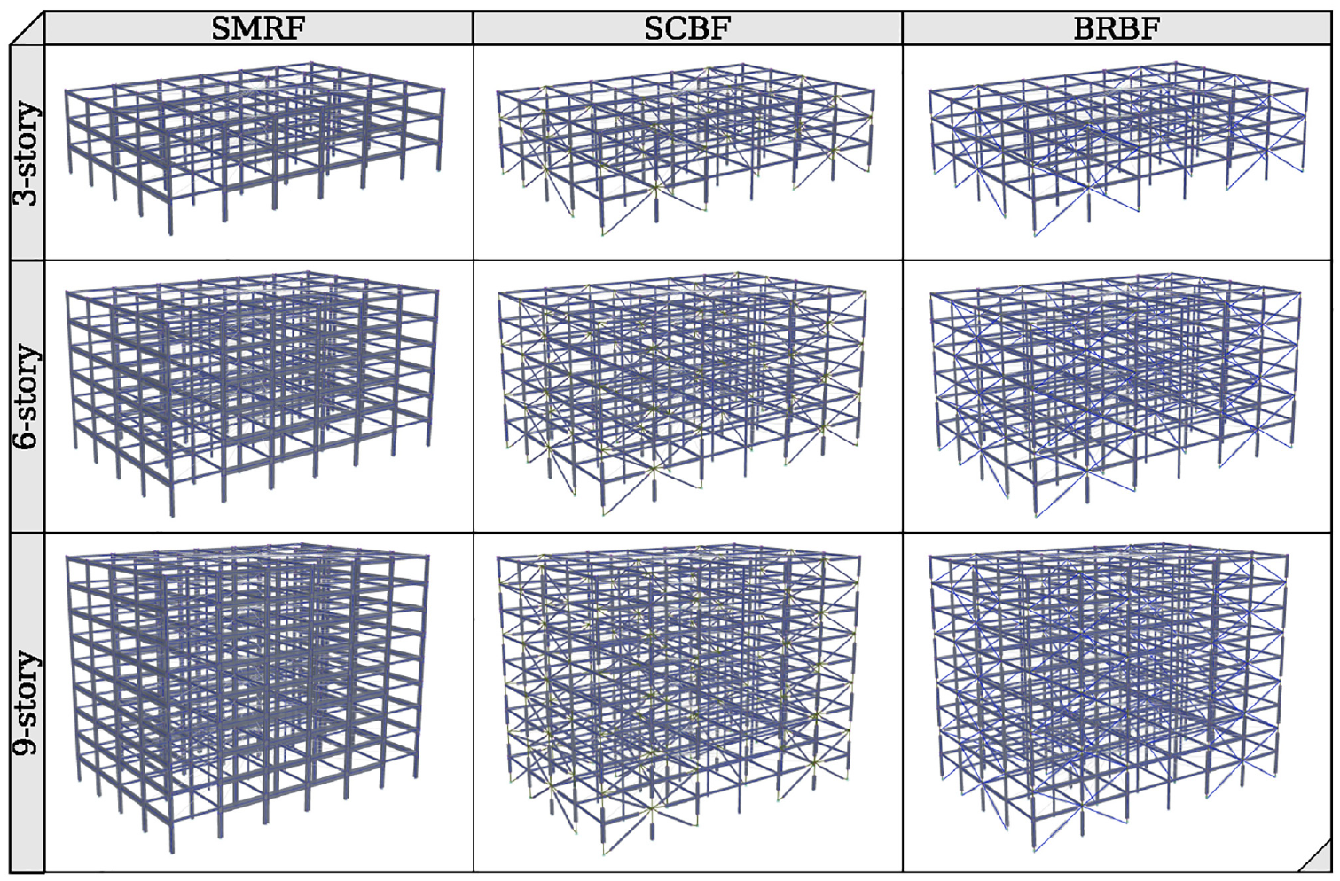
Perspective view of the risk category IV OpenSees models.

Floor diaphragms were assumed to be rigid. The mass and moment of inertia of each story were lumped at a parent node located at the center of mass. Except for the modeling of braces, nonlinear behavior was captured using lumped plasticity principles. We defined assemblies of members with zeroLength elements located at the two ends and employing various uniaxialMaterials at appropriate directions, connected with an elastic beam/column member with modified stiffness properties, as suggested by Zareian and Medina (2010). Since a modified elastic beam/column element was available only for two-dimensional analyses (ModElasticBeam2d), we extended the OpenSees source code to introduce a three-dimensional modified elastic member, ModElasticBeam3d. All column members were assigned the corotational geometric transformation to capture nonlinear geometry effects caused by lateral deformations. Gravity columns were modeled as pinned at the base, while gravity beams were simulated using the Pinching4 uniaxial material assuming a shear-tab connection, implementing what is suggested by Elkady and Lignos (2015). The columns of lateral-load resisting frames were modeled as continuous and fixed at the base.

SMRF columns were modeled using the IMKBilin uniaxial material (November 2022 version), consistent with the approach described by Lignos and Krawinkler (2011). SMRF beams were modeled using the same uniaxial material and accounting for the effects of composite action, drawing on the findings of Elkady and Lignos (2014). The nonlinear behavior of beam-column panel zone joints was simulated by implementing recent recommendations by Skiadopoulos et al. (2021).

SCBF braces were modeled in accordance with what was proposed by Karamanci and Lignos (2014). With this approach, each brace member was simulated using eight displacement-based elements. The elements were placed in the model with a 0.1% initial out-of-plane camber and assigned a corotational geometric transformation to capture their buckling response. Two integration points were used in each element, and their specified fiber-based cross-sections were subdivided with 12 radial sets of three fibers along the thickness. The stress-strain relationship of each fiber was simulated with the Giuffré-Menegotto-Pinto Model (Steel02) combined with Miner’s rule (fatigue) to simulate fracture. The two ends of the braces were connected to zeroLength elements configured to capture the effects of gusset plate yielding, modeled using Steel02, following Hsiao et al. (2012). Rigid offsets were specified to place the gusset plate nonlinear springs at the midpoint of the elliptical clearance region, which was determined during the design process. The chosen configuration results in joints with either present or absent gusset plates. In the former case, such joints were modeled as rigid, assuming the gusset plates would limit panel zone deformations. In the latter case, beam/column joints were modeled similarly to the approach taken for SMRFs. In the case of BRBFs, each brace was modeled using a single corotational truss element, using the general uniaxial material with combined kinematic and isotropic hardening and non-symmetric behavior (Steel4) combined with Miner’s strain accumulation rule to simulate fracture (fatigue), mirroring the parameter calibration procedure of Simpson (2018). BRBFs were assumed to have more compact, rigid gusset plates, and their beams, columns, and their connections were modeled similarly to the SCBFs.

Viscous damping was simulated using the modal damping approach. For each archetype, a damping ratio of 2% $(ζ = 2 %)$ was assigned to the set of low-frequency modes exceeding a 95% contribution to the effective modal mass, in light of recent evidence by Cruz and Miranda (2021). To reduce computational demands, a very small amount of stiffness proportional damping was added to avoid unstable higher mode oscillations while adjusting the modal damping ratios of the lower modes to compensate for its inclusion. In total, 5760 nonlinear time-history analyses were required: one for each combination of hazard level, ground motion, structural system, number of stories, and risk category. The analyses were terminated in cases where the transient drift at any story exceeded 10%, as trial analyses revealed that the rest of the response was characterized by unstable collapse. All analyses either were terminated in this way or successfully converged to their target duration. The significant computational demands of the analyses required for this study were met by utilizing high-performance computing resources provided as a DesignSafe allocation at the Texas Advanced Computing Center (TACC) (Rathje et al. 2017).

Analyzing the structures for a range of hazard levels yielded multiple stripe analysis results, enabling the application of the collapse fragility function fitting approach suggested by Baker (2015). For the collapse fragility function fitting, any analysis resulting in a peak transient drift larger than 6% was treated as an instance of collapse. For the three-story RC IV SMRF archetype no collapse was observed in any hazard level. A 2.5% collapse probability was assigned to hazard level 7, which has an MCE-level return period, motivated by the applicable collapse probability target found in ASCE 7-22. To facilitate a fair comparison of the contribution of the collapse fragility curve dispersion to the losses across different archetypes, the dispersion of the collapse fragility curves was fixed to the commonly used value of 0.4, which is close to the average dispersion observed without enforcing this constraint. The collapse fragility medians are included in Table 3.

Performance Model Identification

We examined two occupancy scenarios, office and an outpatient healthcare facility, similar to what was done in our preliminary study (Vouvakis Manousakis and Konstantinidis 2022) and in the fifth volume of FEMA P-58 (FEMA 2018c). Structural component fragility curves were specified considering the member sizes of each design. Architectural, mechanical, and plumbing components were defined using the types of components and quantities provided by the normative quantity estimation tool of FEMA P-58 (specifically the March 2018 update) for each occupancy scenario (FEMA 2018b). The tool provided a broad list of components, some of which were substituted with their counterpart definitions for applications in high seismic areas whenever those were available. Uncertain component quantities were assumed to follow a lognormal distribution. Aiming to provide insight into the uncertainty deaggregation of the damage and loss estimation process for typical performance evaluations, we considered relatively low levels of uncertainty in the component quantities (lognormal dispersion in the order of 0.15 to 0.35 for most components). Intending to yield results relevant within the context of assessments conducted after making an effort to reduce uncertainty when possible, we only examined two cases of modeling uncertainty, medium and low, using Equation 5-1 of FEMA P-58 volume 1 to obtain the values (FEMA 2018a).

For the definition of tenant equipment and contents, we used the office equipment components available in the FEMA P-58 fragility database and the medical equipment that was used in FEMA P-58 volume 5, implementing the approach followed there for the definition of their median capacity (FEMA 2018c). Their quantities were modified considering the size of the studied archetypes, assuming a department block diagram for a three-story archetype similar to the one in the FEMA report. For the six-story and nine-story archetypes, the tenant equipment and contents were specified by replicating the department blocks of the three-story archetypes across higher stories. While this assumption may compromise realism for the healthcare occupancy scenario, it offers a straightforward approach to achieve a linear relationship between the total square footage and the quantity of each type of equipment, allowing us to compare the performance of the different archetypes with a common baseline. The fragility curves and consequence functions of the medical equipment were defined as outlined in that report. Accordingly, the medians of the fragility curves were estimated using equations provided in the report, and their dispersion was taken as 0.5.

While this study considers RC as a case variable, the goal is to examine how a different RC variant of the same supporting structure would affect the losses for a given performance model. Updating the capacity of the components to reflect an RC IV design would obviously result in fewer realized losses than those of an RC II design for all considered hazard levels. Therefore, we chose to limit the difference to the supporting structure, allowing us to examine if a stronger and stiffer structure would amplify the losses at frequent shaking levels. For this reason, the performance models of RC II versus RC IV cases only differ in terms of the structural fragility curves, which depend on the structural member sections, and RC II should be treated as the baseline case.

The consequences of building replacement were defined by the commonly utilized approach of unit cost estimation. We assumed a replacement cost of USD 250 per square foot for the office occupancy scenario and USD 400 per square foot for healthcare. Replacement time was then estimated by assuming that half of the replacement cost is for labor and dividing the resulting labor cost by USD 700, an assumed daily worker cost, resulting in the expected number of worker days. Multiplying the unit losses by the total square footage resulted in the median replacement loss for each archetype. The replacement time estimation logic presented above follows a pelicun assessment example hosted on DesignSafe (Zsarnóczay and Deierlein 2022). All building replacement loss measures were assumed to be lognormally distributed with a dispersion of 0.35. Considering that the bimodality of the loss distribution can have a strong effect on the breakdown of the contribution of uncertain factors, we also considered two additional cases for the building replacement loss consequences, scaling the medians up and down by 20%. A list of the components present in the performance models can be found in the accompanying online source code repository.

Results

To conduct the performance evaluations, we utilized pelicun (Zsarnóczay et al. 2022), which we extended to support VBSA capabilities. Table 1 summarizes the case variables considered in this work, intending to study their influence on the contribution breakdown of the uncertain factor groups shown in Table 2. Their possible combinations define 6912 individual cases. However, the number of required scenario-based evaluations was 1728 since pelicun can work on multiple decision variables on a single assessment and because the building replacement threshold is considered only during the final stage, when losses are aggregated. Still, the computational demand was substantial since estimating the VBSA sensitivity indices requires results from two baseline assessments and two additional assessments for each uncertain factor group. For each assessment, we generated 10,000 realizations, yielding stable sensitivity index estimates.

Inferring the impact of the case variables on the loss measures and their variance decomposition is done through variable-specific stratification. For any result of interest, we first stratify the data based on the possible values of the examined case variable. We then compare the outcomes between strata, where the influence of the case variable of interest is isolated while the value of other case variables varies freely. A more pronounced interstratal separation suggests that the examined case variable has a large impact on the outcome.

Characteristics of a Performance Evaluation Outcome

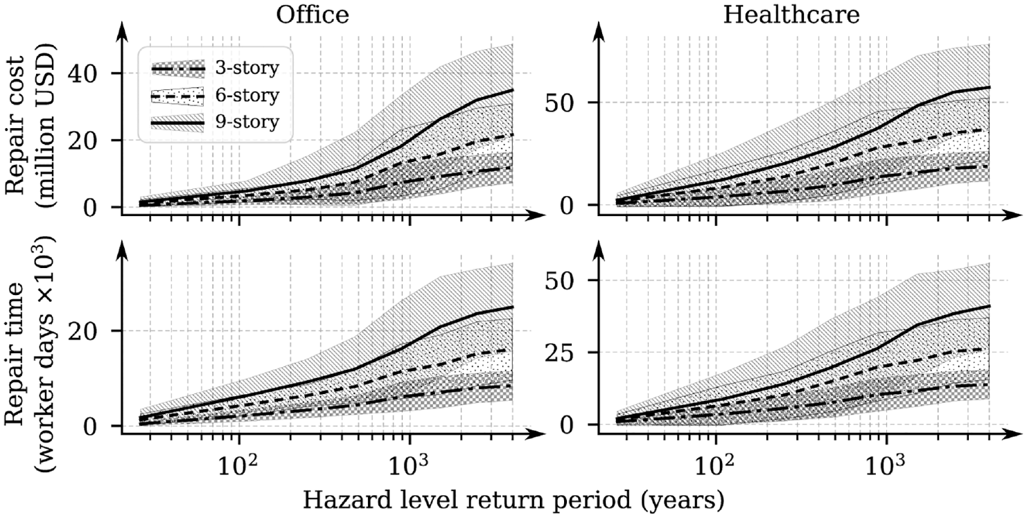
Figure 4 shows the repair cost and sequential repair times as a function of the return period associated with each hazard level. The figure only includes the results for the RC II SMRF archetypes with low modeling uncertainty and a replacement threshold of $c_{R} = 40 %$ , and it would have a similar shape for all other cases. As expected, frequent events result in minimal loss, whereas the losses reach a plateau for rare events driven by the consequences of building replacement. The shaded regions correspond to a range of one standard deviation above and below the mean to illustrate the loss variance we intend to break down.

Figure 4.

Mean ± one standard deviation of loss for the RC II SMRF archetypes. $β_{m} = 0.131$ , $C_{R} = 40 %$ .

Figure 5 shows the cumulative distribution function (CDF) of the repair cost of the nine-story RC II SMRF archetype for each hazard level. The figure reveals how the consequences of building replacement lead to the bimodality of the loss distribution. Separating the cases of building repair versus replacement, the mixture can be broken down into the part driven by the consequences of component damage and the part driven by the consequences of building replacement. This bimodality substantially contributes to the variance of the loss, especially at intermediate hazard levels where it is more pronounced. Bimodality is further amplified with a 40% replacement threshold.

Figure 5.

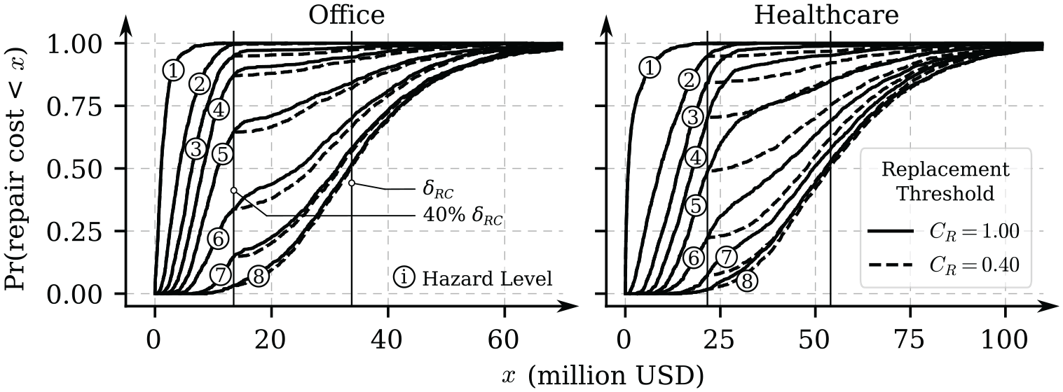
Empirical CDF of loss for each hazard level, corresponding to the SMRF 9 II archetype; δRC: median building replacement cost.

A breakdown of the contribution of different component groups to the loss is shown in Figure 6, where the mean losses of each group, excluding cases of building replacement, are stacked on top of each other for each hazard level. The figure focuses on the nine-story RC II SMRF archetype with low modeling uncertainty and a replacement threshold of 40%. Other cases feature similar relative proportions between the groups. Grouping by component function reveals that the contribution of the occupant-eq6-and-contents (EC) group—which includes occupancy-specific components, such as workstations for office and medical equipment for healthcare—is large for all hazard levels and larger for the healthcare occupancy scenario. Grouping by EDP type shows that the majority of component-driven losses are attributed to acceleration-sensitive components in both occupancy scenarios. Although not shown, this finding is consistent across all examined cases, challenging the common engineering practice of advocating for stiffer structural systems to improve performance by reducing damage to drift-sensitive components.

Figure 6.

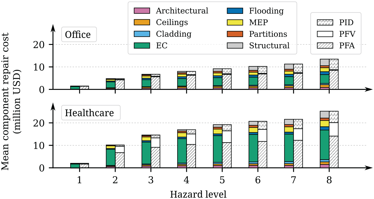
Loss breakdown by component group for realizations excluding building replacement. Nine-story RC II SMRF archetypes, $β_{m} = 0.131$ , $C_{R} = 40 %$ . MEP: mechanical/electrical/plumbing; EC: occupancy-specific equipment and contents.

Effect of Case Variables on Loss

Before studying the contribution of each uncertain factor group to the loss variance, we begin by examining the impact of the case variables on the mean loss. Figure 7 shows the stratification of a subset of the results corresponding to the repair cost of three-story office archetypes. We observed the same trend regardless of the decision variable, occupancy, or number of stories, obviating the need to include more cases in the strata. Stratifying by structural system reveals how a stiffer system, like SCBFs resulted in higher losses for frequent earthquakes, while the more flexible SMRFs performed worse at the higher end of shaking intensity. A similar observation is made with RC, where RC IV structures yielded higher losses than RC II for low values of IM with a reversal for higher IM values, revealing that an over-designed supporting structure without any intervention on the nonstructural components is not sufficient for better performance across all levels of shaking. The median loss only becomes higher for the RC II case starting from hazard level 4, which has a design-level return period. This finding is in agreement with the observations reported by Issa et al. (2023) regarding the effects of the importance factor on nonstructural component performance. In the case of modeling uncertainty, $β_{m}$ , we see that compared with low (L), a medium level (M) amplifies the losses for hazard level 1, while it has no effect at hazard level 8. Modeling uncertainty inflates the marginal variance of the EDPs, which are lognormally distributed, and thus increases their mean, leading to more component damage and higher losses. At the highest hazard level, losses are predominantly driven by building replacement, and in this case, the influence of modeling uncertainty is diminished. The effect of the replacement threshold, $C_{R}$ , is minimal at the lowest hazard levels, where component losses rarely trigger building replacement. The effect becomes substantial at higher hazard levels, with a 40% replacement threshold driving up the losses by triggering more instances of building replacement.

Figure 7.

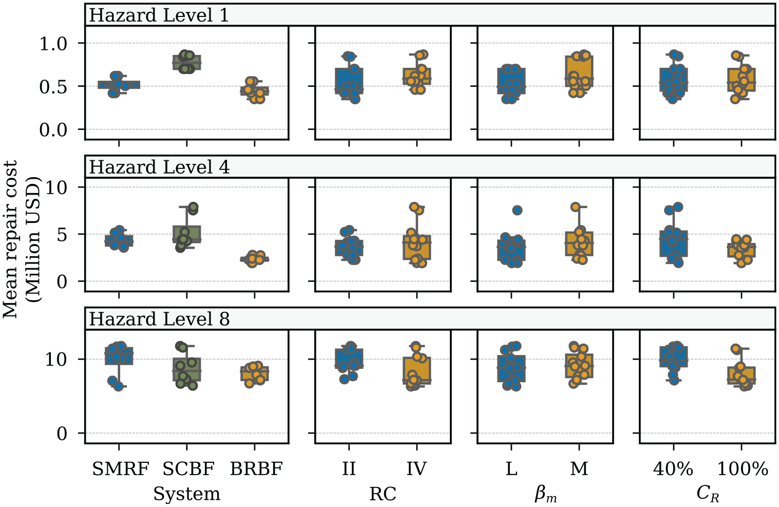
Repair cost group average for the 3-story office archetypes. Grouping is done by structural system, risk category RC, modeling uncertainty $β_{m}$ , and replacement threshold $C_{R}$ .

The marginal variance of the EDPs is a driving factor of the effect of the case variables on the uncertain factor contributions to the loss variance. While those marginal variances are not affected by certain case variables, they are affected by the hazard level, the structural system, the number of stories, and the risk category. Figure 8 demonstrates these effects utilizing the previously discussed variable-specific stratification for the marginal logarithmic standard deviation (or dispersion) of the distribution of PFAs, PFVs, and PIDs. The dispersion of all EDPs is very sensitive to the modeling uncertainty since it directly amplifies their initial dispersion. Being more influenced by higher-mode effects, PFAs are sensitive to the hazard level and the number of stories, while other attributes have a smaller effect.

Figure 8.

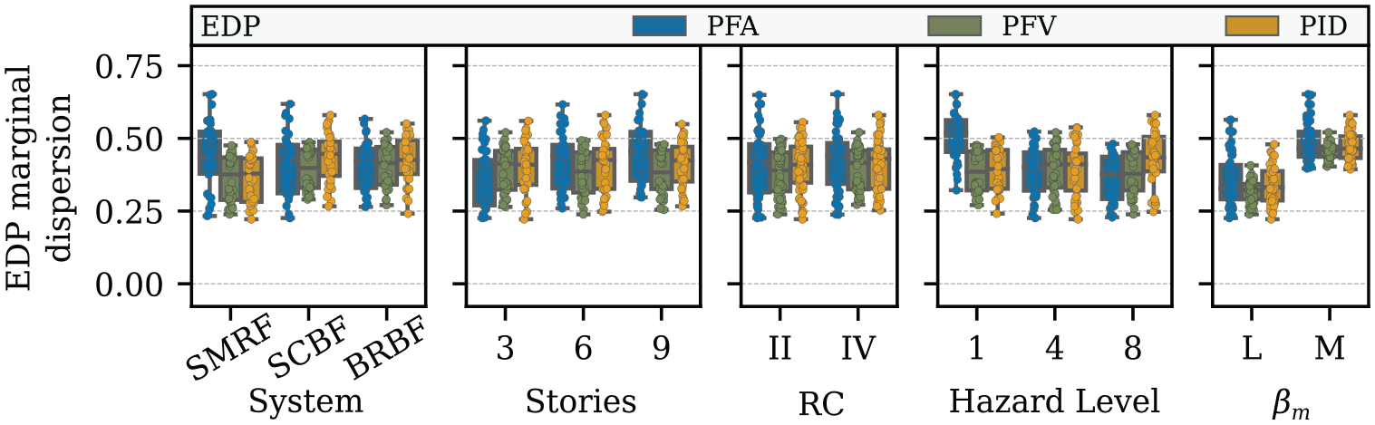
Effect of case variables on the EDP marginal dispersion.

Variance-Based Sensitivity Analysis Results

Figure 9 presents the first-order and the total-effect sensitivity indices for the subset of cases with RC II archetypes, low modeling uncertainty $(β_{m} = 0.131)$ , and a replacement threshold of 40%, for hazard levels 1, 4, and 8. Notable trends emerging from the figure include the significant contribution of the EDP uncertain factor group to the loss variance for hazard levels 1 and 4. As discussed earlier, higher values indicate a strong contribution to the variance of the result. The values associated with the EDP group remain high until uncertain factors related to building replacement take precedence: B-DM and B-DV. In most cases, the C-DM group has a smaller contribution than the EDP group, only surpassing it for the very small subset of three-story healthcare archetypes. The C-Q and C-DV uncertain factor groups were excluded from the figure because their influence on the loss variance was minimal.

Figure 9.

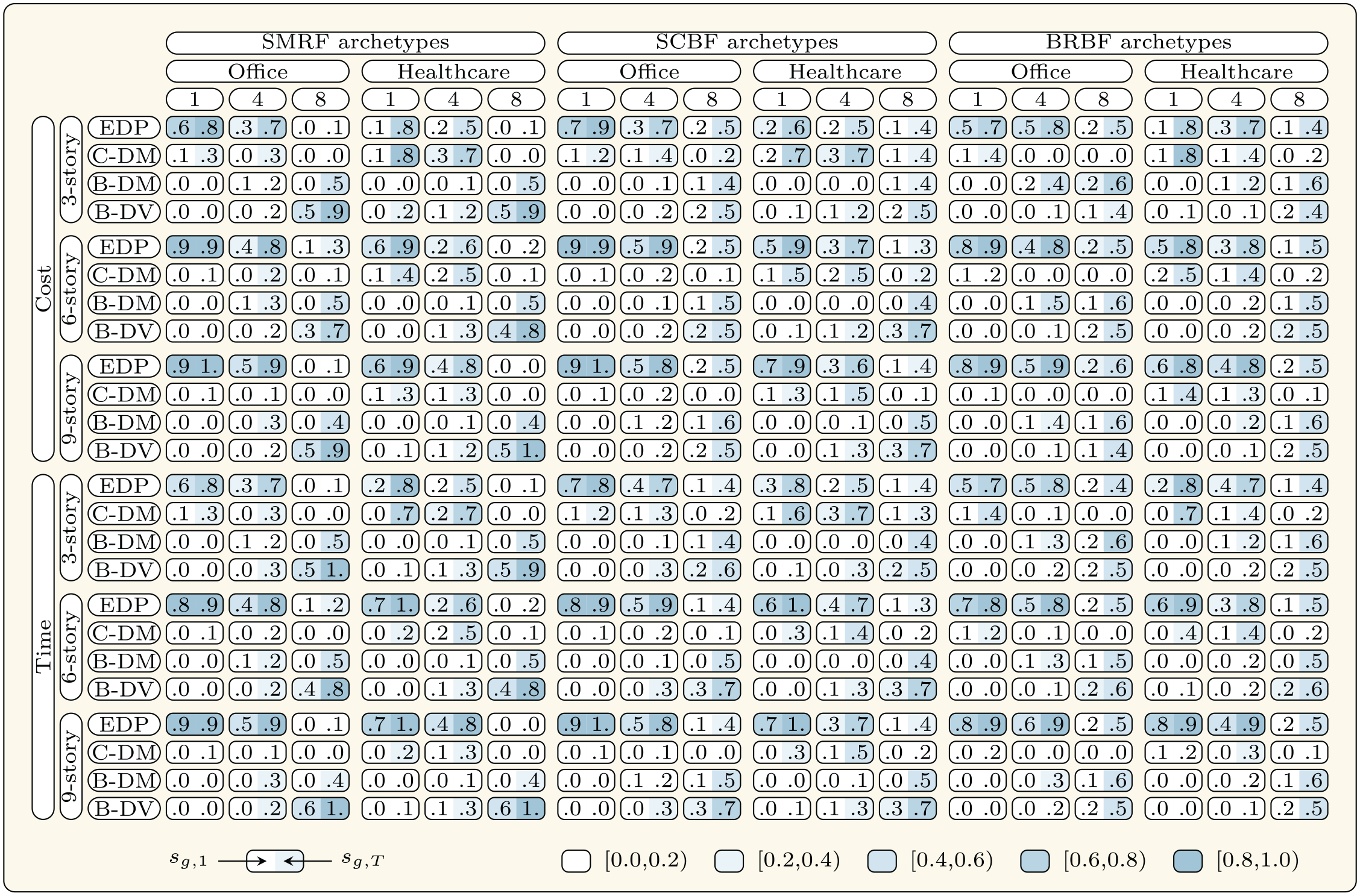
First-order and total-effect sensitivity indices for RC II archetypes, $β_{m} = 0.131$ , $C_{R} = 40 %$ .

Building replacement, triggered at higher hazard levels, strongly affects the breakdown of the uncertain factor contributions to the loss variance. A higher likelihood of building replacement amplifies the contribution of uncertain factors associated with the distinction of building replacement cases at the expense of other uncertain factor contributions. Generally, for any given hazard level, all sensitivity indices are normalized against the same loss variance, and therefore, if one is relatively high, the rest are smaller. In other words, artificially increasing the marginal variance of a given uncertain factor group would increase its sensitivity indices and lower the indices of all other groups. Evidenced by the fact that the total-effect sensitivity index is higher than the first-order index in most cases, Figure 9 indicates the presence of higher-order interactions for all uncertain factor groups. Higher-order interactions imply that the effect of a random factor on the estimated loss measure variance depends on the value of other uncertain factors. This is not surprising, given the nonlinear nature of the damage and loss estimation framework. In practice, this means that ignoring the higher-order interactions can lead to incorrect conclusions on the relative importance of random factors. Figure 9 also demonstrates that different case variables can affect the variance breakdown, which we examine next.

In Figure 10, we utilize variable-specific stratification to all total-effect sensitivity indices obtained in this study. The figure is structured with columns corresponding to hazard levels 1, 4, and 8, and rows corresponding to the rest of the case variables defined in Table 1. In each subplot and for every uncertain factor group, all available data are stratified based on the value of the case variable and plotted in the form of a group of boxplots. The figure confirms the dependence of the variance contribution breakdown with hazard level, primarily driven by building replacement, as discussed previously: the contribution of uncertain factor groups associated with building replacement (B-DM, B-DV) is amplified as the hazard level increases, with the opposite being true for the component-related groups (C-Q, C-DM, C-DV). The fact that the EDP group remains relevant at the highest hazard levels suggests that it contains uncertain factors that influence the occurrence of building replacement events.

Figure 10.

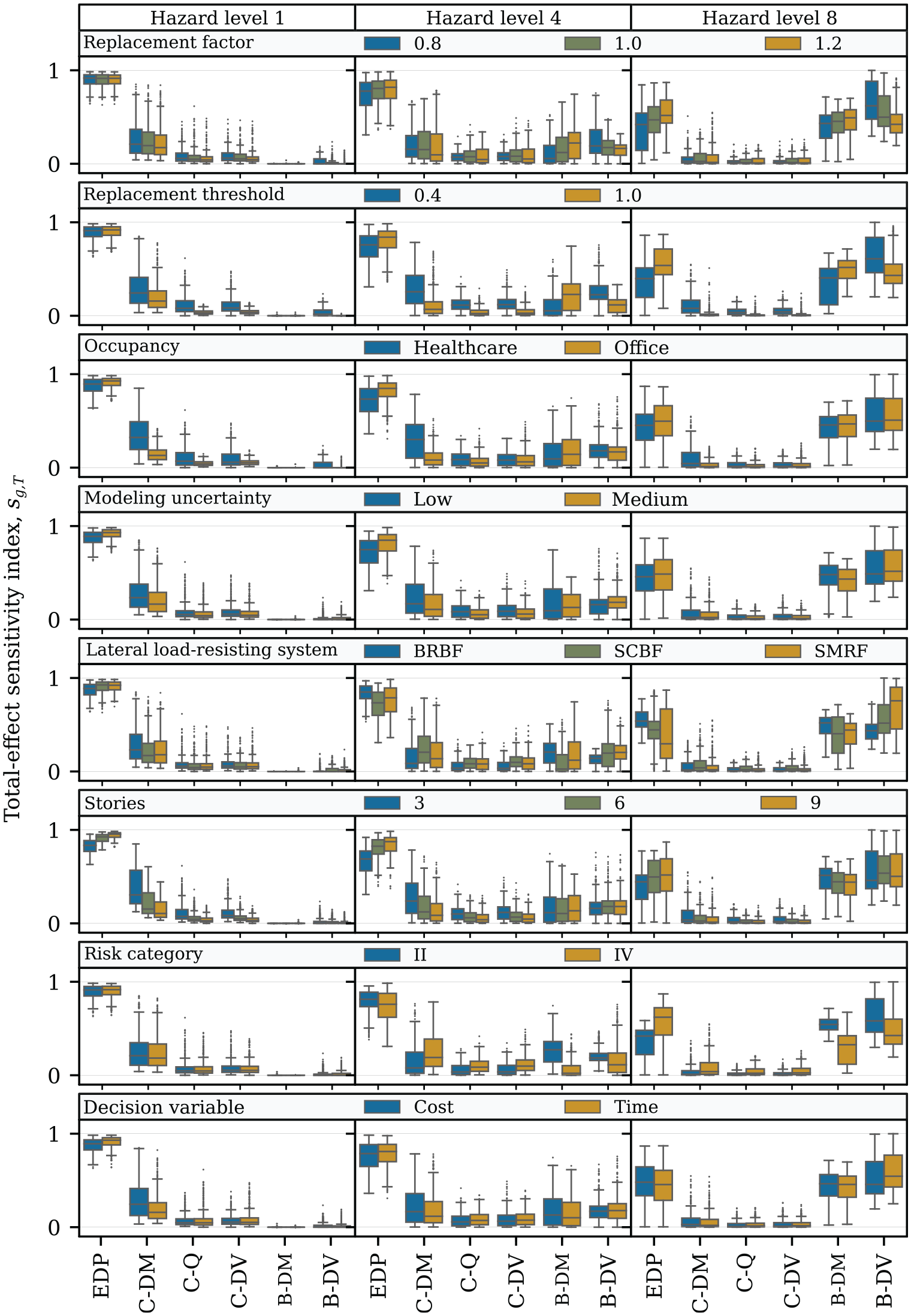
Total-effect sensitivity indices of uncertain factor groups stratified by each case variable.

Examining different cases for the magnitude of the building replacement consequences, we observe changes in the loss variance breakdown, even when the variance of the inputs remains unchanged. This is caused by the losses associated with cases of building replacement versus building repair getting closer together or further apart, affecting the overall loss variance as well as the contribution of each uncertain input. The building replacement threshold can also greatly affect the contribution breakdown, with a lower threshold resulting in more building replacement cases driven by component-related uncertain factors, contrary to excessive drift or collapse. Compared with those building replacement triggering events, excessive component cost is associated with the component related uncertain factors. Therefore, a value of 40% increases their influence on the variance of the loss. More cases of building replacement resulting from a 40% replacement threshold also amplify the contribution of the B-DV group, further reducing the influence of the B-DM group.

Stratifying by occupancy, we observe how the high-dispersion fragility curves and the larger consequence uncertainty in the healthcare components amplify the contribution of the C-DM group. Modeling uncertainty has a direct impact on the EDP marginal variance and no effect on any other uncertain factor. Accordingly, we observe an increase in the contribution of the EDP group with medium modeling uncertainty, attributed to the larger EDP marginal variance that can also be seen in Figure 8.

Since all considered structural system configurations were designed for the same site, stratifying by different structural systems does not strongly affect the collapse probability. However, it still affects the marginal variance of different kinds of EDPs and the likelihood of excessive residual drifts triggering building replacement.

There is a notable effect in the contribution breakdown when stratifying the data by the number of stories. As the number of stories increases, the contribution of the EDP group is amplified at the expense of the other groups. This is partly due to the more considerable PFA marginal variance of the taller structures, shown in Figure 8. Another potential driving factor of this effect is the differences between the performance models for structures with different numbers of stories, all else being equal. While the building replacement consequences and the quantities of most components scale linearly with the number of stories, higher structures feature fewer units of certain mechanical, electrical, and plumbing components, such as elevators, chillers, and cooling towers, than what a linear interpolation would require. These components, however, are responsible for only a small proportion of the total component repair cost.

While the effect of the risk category is small at the lower hazard levels, where the buildings respond primarily elastically, it becomes more prominent at higher hazard levels. RC IV cases result in fewer instances of building replacement. Therefore, the B-DM and B-DV groups have a lower contribution, which in turn amplifies the contribution of the rest of the groups. Finally, comparing the results for either cost or time, we find that uncertain factors contribute similarly to the estimation variance.

From a factor prioritization standpoint, we identify EDP, C-DM, B-DM, and B-DV as the most influential uncertain factor groups, with C-Q and C-DV having less influence on the variance of the estimated loss. In Figure 11, we closely examine those high-contributing groups by partitioning their contents. The EDP group is broken down into four subgroups based on EDP type: PFA, PFV, PID, and RID. This partitioning reveals that compared with PID or PFV, PFA has a substantially larger influence on the variance of the loss. There are several potential reasons behind this, including the large proportion of the loss driven by acceleration-sensitive components, the fact that damage initiation of drift-sensitive components begins at higher hazard levels where building replacement is likely, and the higher marginal variance of the PFA at lower hazard levels. At higher hazard levels, RID becomes a substantial contributor, surpassing the contribution of PFA. RIDs are used as an input to the excessive drift fragility curves of the building, which trigger building replacement. Therefore, the uncertainty associated with RIDs is expected to become an important contributor to the loss variance at high hazard levels.

Figure 11.

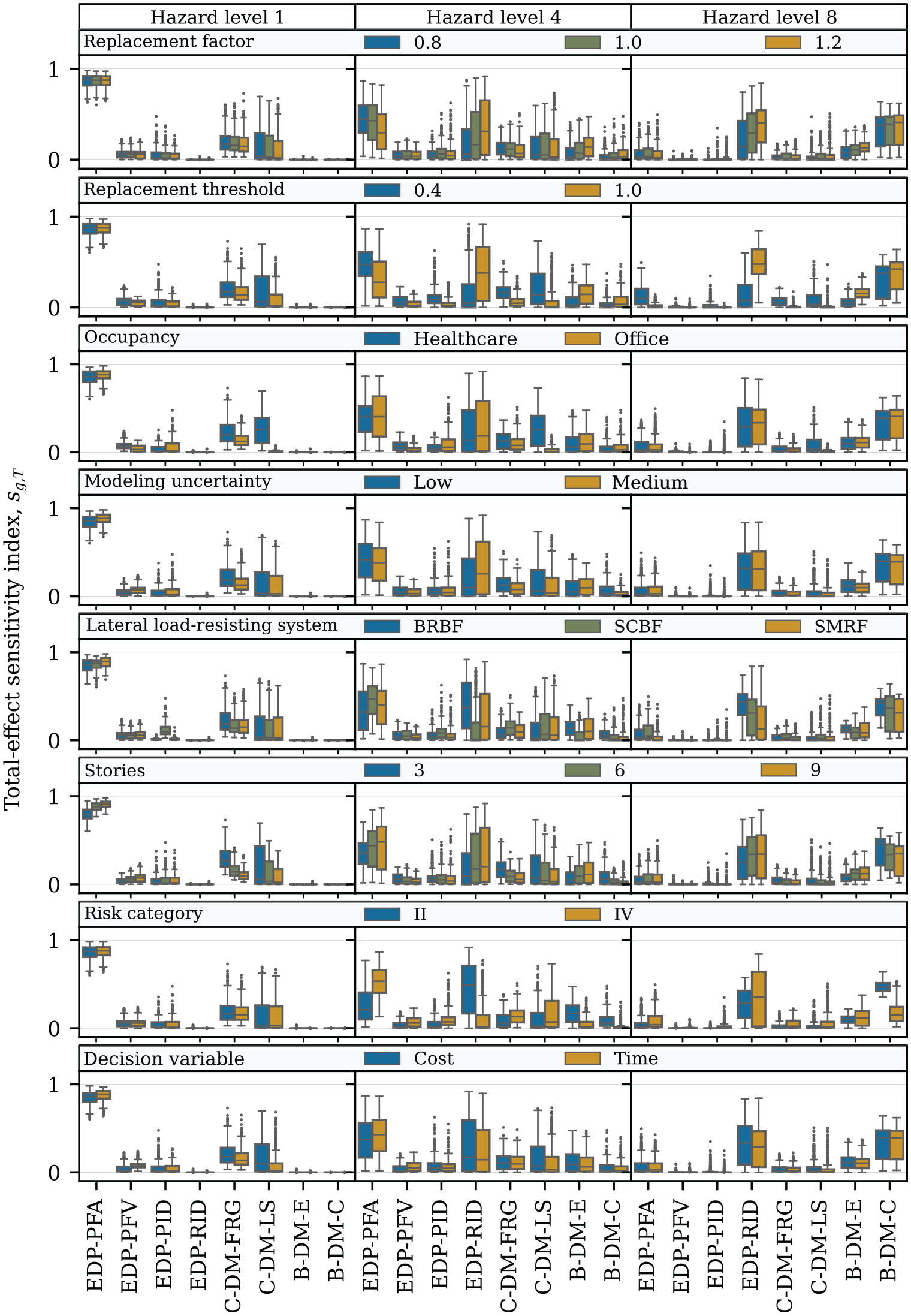
Total-effect sensitivity indices of uncertain factor subgroups stratified by each case variable.

The C-DV group is broken down into the capacity of the components, C-DM-FRG, and the realized consequence, C-DM-LS. The capacities of the components is defined by their fragility curves, and their uncertainty is simulated with their associated dispersion. When a damage state is reached, there can be a single consequence, in which case there is no uncertainty in the realized consequence or one of multiple possible consequences with different associated losses. In the latter case, a probability is assigned to each potential consequence, and loss uncertainty is introduced through the resulting multinomial consequence distribution. C-DM-LS captures the uncertain factors involved with determining the realized consequence. Stratifying the sensitivity indices by occupancy reveals that the C-DM-LS subgroup appears to substantially contribute to the loss variance for the healthcare occupancy scenario. This results from the highly uncertain damage consequences defined for the medical equipment and contents. Per FEMA P-58 volume 5, upon damage, those components are assumed to be repairable at a 10% replacement loss with a probability of 80% or damaged beyond repair at a 100% replacement loss with a probability of 20%.

Finally, the B-DM group is broken down into the uncertain factor associated with the building’s collapse fragility curve, B-DM-C, and the building’s excessive residual drift fragility curve, B-DM-E. The influence of both subgroups at low hazard levels is minimal since collapse or excessive drift is improbable. At higher hazard levels, comparing the two suggests that uncertainty associated with the building’s collapse fragility curve contributes more to the loss variance, but this direct comparison is misleading. These two subgroups are exclusively associated with the uncertain capacity defined by the fragility curves without accounting for the uncertainty in their inputs. Given that the assessments utilize CS as target spectra, the input to the building’s collapse fragility curve for any given hazard level has no variance. In contrast, the inputs to the building’s excessive drift fragility curves come from the EDP-RID group, which considerably contributes to the loss variance.

Figures 12 and 13 offer an alternative, more in-depth view of the interplay between different uncertain factor groups and their respective contributions to loss variance. Focusing on a pair of uncertain factor groups, we visualize their total-effect sensitivity indices for each analysis unit represented as a point on a scatter plot, where the size of the point represents the hazard level, and the hue partitions them based on an additional case variable. Figure 12b illustrates the increase in relevance of the C-DM group for the healthcare occupancy, reducing the relevance of the EDP group. At larger hazard levels, the relevance of both EDP and C-DM is reduced in favor of the groups associated with building replacement, B-DV, and B-DM, as shown in Figure 12a. Considering the B-DV–B-DM pairs shown in Figure 12c, we observe a reduction in the relevance of the B-DM group for RC IV archetypes. Both RC variations have the same replacement loss variance. Therefore, the difference can be attributed to the larger capacity of their collapse fragility curve and the reduced values of the RIDs. When partitioning the C-DM–B-DM pairs by occupancy (see Figure 12d), we observe that the C-DM group has a higher contribution for healthcare, and for both occupancy scenarios, the contribution of C-DM decreases at higher hazard levels in favor of B-DM.

Figure 12.

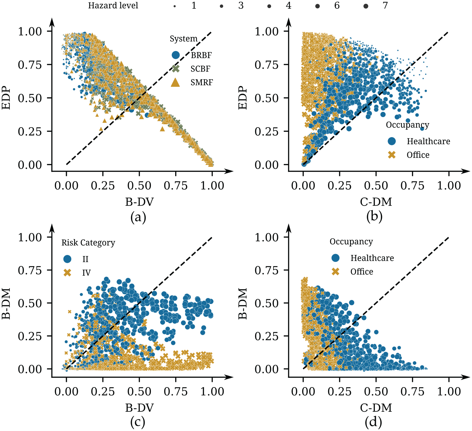
Total-effect sensitivity indices of uncertain factor group pairs: (a) EDP vs. B-DV, (b) EDP vs. C-DM, (c) B-DM vs. B-DV, and (d) B-DM vs. C-DM.

Figure 13.

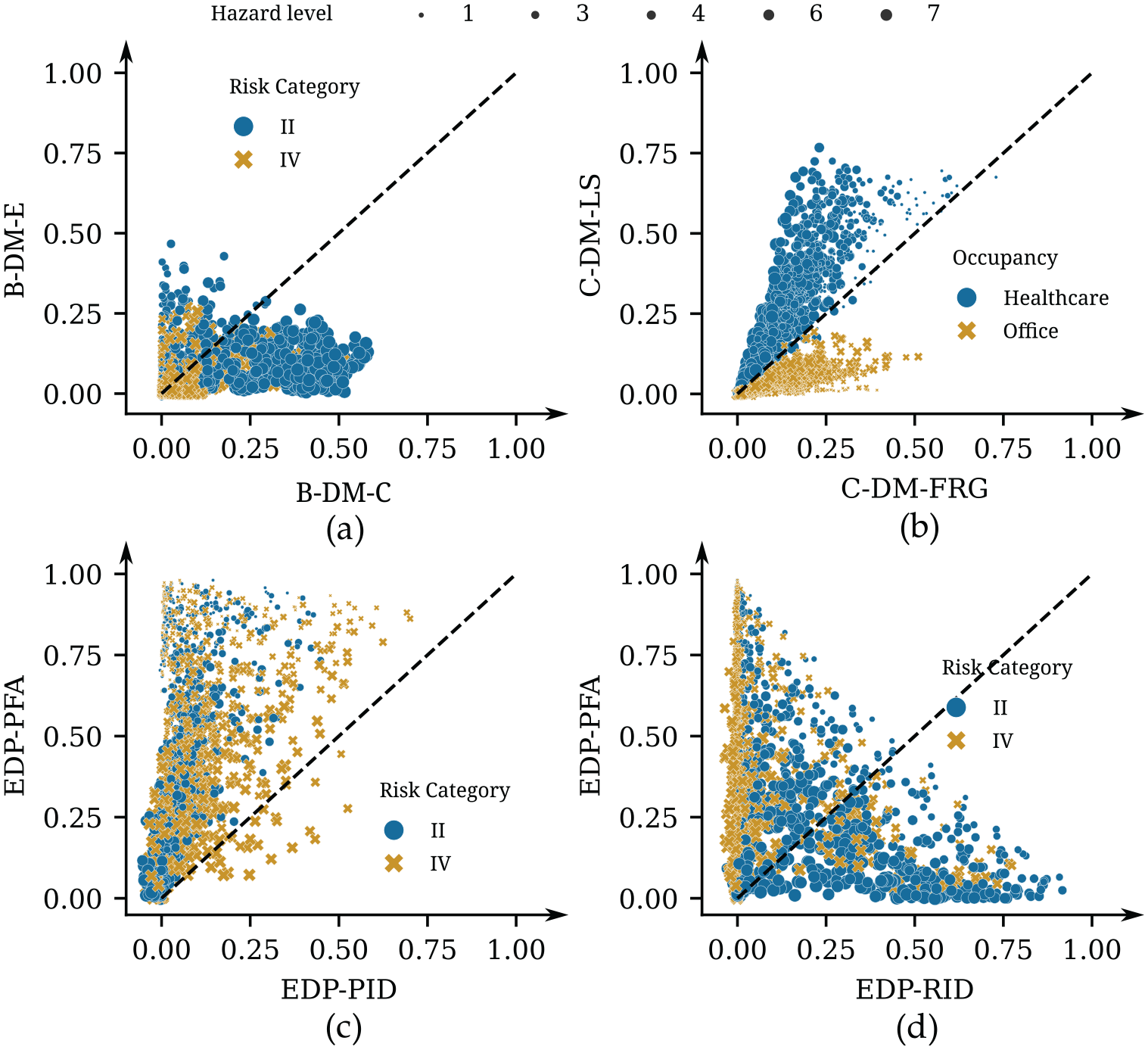
Total-effect sensitivity indices of uncertain factor subgroup pairs: (a) B-DM-E vs. B-DM-C, (b) C-DM-LS vs. C-DM-FRG, (c) EDP-PFA vs. EDP-PID, and (d) EDP-PFA vs. EDP-RID.

Figure 13 concerns the uncertain factor group subcomponents introduced in Figure 11. Compared with RC II, results from RC IV archetypes suggest a reduction in the influence of both the B-DM-E and B-DM-C subgroups. In contrast, the B-DM-C subgroup has a larger influence on RC II archetypes at higher hazard levels (see Figure 13a). Partitioning the C-DM-FRG–C-DM-LS pairs by occupancy reveals the increase in relevance of theC-DM-LS subgroup when highly uncertain consequence functions are utilized, while its relevance is relatively smaller otherwise, as shown in Figure 13b. While the EDP-PFA group has a substantial influence in general, there are instances of certain RC IV archetypes where the EDP-PFA and the EDP-PID groups have a similar contribution, especially at higher hazard levels, even though the influence of both groups is minimized at those levels (see Figure 13c). Finally, Figure 13d partitions the EDP-PFA–EDP-RID pairs by risk category, revealing a general tendency for EDP-RID to have a larger impact on the loss measure variance for RC II archetypes.

Summary and Conclusions

In this study, we utilized variance-based sensitivity analysis (VBSA) within the framework of intensity-based FEMA P-58 assessments to examine the relative contribution of uncertain factors that are part of the framework to the variance of the estimated losses. We partitioned all uncertain factors into groups based on their purpose in the damage and loss estimation framework and examined the relative contributions of those groups to the losses generated for a diverse set of cases.

The results demonstrate a consistent dependence of the contribution breakdown to the hazard level, with uncertain factors associated with component damage having a larger influence at low levels of shaking and building-specific uncertain factors gaining influence at higher levels, driven by the increase in the likelihood of building replacement. For all of the considered cases, uncertain factors associated with uncertain component quantities and component-driven losses conditioned on their realized damage consequences had the lowest impact on the estimated loss variance. A breakdown of the uncertain factor groups into subcomponents revealed that PFAs consistently had the largest influence among all uncertain factors at lower hazard levels, with RIDs, building fragility curves, and replacement losses contributing the most at high hazard levels.

By dissecting the data with variable-specific stratification, we demonstrated the effects of various case variables, which are summarized in Table 1, on the relative contributions of the uncertain factor groups shown in Table 2. The results show how these variables influence the importance of the uncertain factor groups across hazard levels. The EDP group consistently had a high contribution at lower shaking intensities. At higher hazard levels, the highest contributing uncertain factor group strongly depended on the replacement threshold, risk category, and structural system. The relative contribution of component-related uncertainties varied with all examined case variables, being higher for cost estimates, the healthcare occupancy scenario, low modeling uncertainty, a 40% replacement threshold, RC IV, and shorter archetypes.

Directly applying variable-specific stratification to the mean losses produced insightful incidental findings. We examined the relative performance of different lateral load-resisting systems and risk categories, revealing how stiffer systems like SCBFs led to higher losses at frequent earthquake levels, while the more flexible SMRFs showed increased losses at higher shaking intensities. A similar observation was made for the effect of the risk category of the supporting structure given the same nonstructural components: RC IV structures resulted in higher losses at low shaking intensities but performed better at higher intensities. We examined the role of modeling uncertainty, demonstrating that increased modeling uncertainty leads to higher loss estimates, especially at lower hazard levels. Similarly, a lower building replacement threshold increased loss estimates at higher hazard levels due to the increase in the likelihood of building replacement. These observations highlight the importance of properly defining the value of these two case variables; otherwise, the resulting loss estimates can be biased.

The results of this study are limited to intensity-based assessments. Future research can focus on prioritizing uncertain factors associated with time-based assessment outcomes. Rare earthquakes lead to higher losses primarily due to building-specific uncertain factors, whereas more frequent earthquakes result in lower losses, largely driven by component-specific uncertain factors. Factor prioritization could summarize the overall contribution of each uncertain factor, integrating over all return periods while also including the uncertainty associated with the site’s seismic hazard.

Considering the differences in the contribution breakdown observed for the two examined occupancy scenarios, it becomes clear that the performance model has a large impact on factor prioritization. For example, a performance model involving a large number of easily damaged drift-sensitive components that lead to large losses and fewer acceleration-sensitive components would result in a different prioritization of each EDP type. In addition, drawing broad factor prioritization conclusions based on the results of this study should be done with caution, as it is not immediately clear how the results could be affected by unexamined case variables, such as site seismicity. In any given case, it is safest to conduct VBSA with the particular inputs at hand rather than rely solely on the insight gained from our results.

Behind the prioritization offered in this study lies an assumption that the specified probability distributions of all associated uncertain factors represent our best state of knowledge. It is easy, however, to argue against that, especially regarding the crudely defined component-related uncertain factors. Before accepting that component-related uncertain factors have a small contribution to the loss variance, one should reexamine the approach taken to define their damage and loss distribution parameters and whether the simulated component loss realizations truly capture the overall real-world uncertainty associated with their performance.

Based on the findings of this study, analysts tasked with the application of a loss estimation should begin by carefully examining and scrutinizing the input parameters for the distributions of all associated uncertain factors. Attempting to reduce uncertainty without first ensuring that the initial inputs are robust will inadvertently lead to biased results. As a next step, the case variables, such as the modeling uncertainty and the replacement threshold, should be clearly defined. If, after taking these steps, there is the desire to reduce the uncertainty of the estimated losses, considering the persistent relevance of the EDP group to the loss variance across hazard levels, a crucial step is to develop a high-fidelity model and gain confidence in the realism of the modeling parameters used. This can help justify a smaller modeling uncertainty value, directly reducing the EDP marginal variance while also reducing bias in the estimated EDPs. Such a model can also improve the accuracy of the estimated residual drifts and aid in the definition of a collapse fragility curve with less dispersion. Both of these sources of uncertainty emerged as highly relevant at higher intensity levels. VBSA can then be applied to reveal potentially viable candidates for further variance reduction.

In conclusion, by applying VBSA within the FEMA P-58 framework, our study has demonstrated the effect of a variety of case variables on the relative contributions of uncertain factors, enhancing the understanding of the predominant sources of uncertainty and the extent to which the breakdown can change depending on the case at hand. It serves as a valuable resource for future studies aiming at enhancing the reliability of seismic risk estimation.

Supplemental Material

sj-pdf-1-eqs-10.1177_87552930241291073 – Supplemental material for Factor Prioritization in FEMA P-58 Loss Estimation

Supplemental material, sj-pdf-1-eqs-10.1177_87552930241291073 for Factor Prioritization in FEMA P-58 Loss Estimation by Ioannis Vouvakis Manousakis and Dimitrios Konstantinidis in Earthquake Spectra

Footnotes

Acknowledgements

We would like to thank Alan Kren for his insightful input and guidance in the archetype design phase of our research. His extensive experience in structural design helped us arrive at realistic archetype designs. We are also grateful for Dr. Kevin Milner’s support with OpenSHA, and we thank Dr. Adam Zsarnóczay, Prof. Barbara Simpson, and Prof. Dimitrios Lignos for their insightful suggestions throughout the various stages of this work. This research utilized resources of the Frontera computing project at the Texas Advanced Computing Center (Stanzione et al. 2020). Frontera is made possible by National Science Foundation award OAC-1818253.

Declaration of Conflicting Interests

The author(s) declared no potential conflicts of interest with respect to the research, authorship, and/or publication of this article.

Funding

The author(s) received no financial support for the research, authorship, and/or publication of this article.

ORCID iDs

Ioannis Vouvakis Manousakis

Dimitrios Konstantinidis

Research Data and Code Availability

The source code reproducing the results presented in this study is available in an online repository (Vouvakis Manousakis 2024). The repository contains instructions on reproducing or directly obtaining the analysis results.

Supplemental Material

Supplemental material for this article is available online.

References

American Institute of Steel Construction (AISC) (2016a) Prequalified Connections for Special and Intermediate Steel Moment Frames for Seismic Applications (AISC 358-16). Chicago, IL: AISC.

American Institute of Steel Construction (AISC) (2016b) Seismic Provisions for Structural Steel Buildings (AISC 341-16). Chicago, IL: AISC.

American Institute of Steel Construction (AISC) (2016c) Specification for Structural Steel Buildings (AISC 360-16). Chicago, IL: AISC.

American Society of Civil Engineers (ASCE) (2022) Minimum Design Loads and Associated Criteria for Buildings and Other Structures (ASCE/SEI 7-22). Reston, VA: ASCE.

Aslani

Cabrera

Rahnama

(2012) Analysis of the Sources of Uncertainty for Portfolio- Level Earthquake Loss Estimation. Earthquake Engineering & Structural Dynamics 41(11). DOI:10.1002/eqe.2230.

Baker

(2015) Efficient analytical fragility function fitting using dynamic structural analysis. Earthquake Spectra 31(1). DOI:10.1193/021113EQS025M.

Baker

Lee

(2018) An improved algorithm for selecting ground motions to match a conditional spectrum. Journal of Earthquake Engineering 22(4). DOI:10.1080/13632469.2016. 1264334.

Baker

Lin

Haselton

(2014) Ground motion selection for performance-based engineering: effect of target spectrum and conditioning period. In: Fischinger

(ed.) Performance-Based Seismic Engineering: Vision for an Earthquake Resilient Society, Geotechnical, Geological and Earthquake Engineering. Dordrecht, Netherlands: Springer. DOI:10.1007/978-94-017-8875-528.

Bozorgnia

, et al. (2014) NGA-West2 Research Project. Earthquake Spectra 30(3). DOI: 10.1193/ 072113EQS209M.

10.

Bradley

(2013) A critical examination of seismic response uncertainty analysis in earthquake engineering. Earthquake Engineering & Structural Dynamics 42(11). DOI: 10.1002/eqe.2331.

11.

Cook

Liel

Haselton

Koliou

. (2022) A framework for operationalizing the assessment of post-earthquake functional recovery of buildings. Earthquake Spectra 38(3). DOI:10.1177/ 87552930221081538.

12.

CoreBrace (2020) Bolted Brace Design Guide. URL https://corebrace.com/ resources/design-aid/.

13.

Cremen

Baker

(2021) Variance-based sensitivity analyses and uncertainty quantification for FEMA P-58 consequence predictions. Earthquake Engineering & Structural Dynamics 50(3). DOI:10.1002/eqe.3370.

14.

Cruz

Miranda

(2021) Damping ratios of the first mode for the seismic analysis of buildings. Journal of Structural Engineering 147(1). DOI:10.1061/(ASCE)ST.1943-541X.0002873.

15.

Elkady

Lignos

(2014) Modeling of the composite action in fully restrained beam-to-column connections: Implications in the seismic design and collapse capacity of steel special moment frames. Earthquake Engineering & Structural Dynamics 43(13). DOI: 10.1002/eqe.2430.

16.

Elkady

Lignos

(2015) Effect of gravity framing on the overstrength and collapse capacity of steel frame buildings with perimeter special moment frames. Earthquake Engineering & Structural Dynamics 44(8). DOI:10.1002/eqe.2519.

17.

Federal Emergency Management Agency (FEMA) (2018a) Seismic Performance Assessment of Buildings, Volume 1 – Methodology, Second Edition. Washington, D.C.: FEMA.

18.

Federal Emergency Management Agency (FEMA) (2018b) Seismic Performance Assessment of Buildings, Volume 3 – Supporting Electronic Materials and Background Documentation, Third Edition. Washington, D.C.: FEMA.

19.

Federal Emergency Management Agency (FEMA) (2018c) Seismic Performance Assessment of Buildings, Volume 5 – Expected Seismic Performance of Code-Conforming Buildings. Washington, D.C.: FEMA.

20.

Field

Jordan

Cornell

(2003) OpenSHA: A developing community-modeling environment for seismic hazard analysis. Seismological Research Letters 74(4). DOI: 10.1785/ gssrl.74.4.406.

21.

Field

Milner

Porter

(2020) Assessing the value of removing earthquake-hazard-related epistemic uncertainties, exemplified using average annual loss in California. Earthquake Spectra 36(4). DOI:10.1177/8755293020926185.

22.

Field

, et al. (2014) Uniform California Earthquake Rupture Forecast, Version 3 (UCERF3)—the time-independent model. Bulletin of the Seismological Society of America 104(3). DOI: 10.1785/0120130164.

23.

Hsiao

Lehman

Roeder

(2012) Improved analytical model for special concentrically braced frames. Journal of Constructional Steel Research73. DOI:10.1016/j.jcsr.2012.01.010.

24.

Iervolino

(2017) Assessing uncertainty in estimation of seismic response for PBEE. Earthquake Engineering & Structural Dynamics 46(10). DOI:10.1002/eqe.2883.

25.

Issa

Silva-Lopez

Baker

Burton

. (2023) Machine-learning-based optimization framework to support recovery-based design. Earthquake Engineering & Structural Dynamics 52(11). DOI:10.1002/eqe.3860.

26.

Karamanci

Lignos

(2014) Computational approach for collapse assessment of concentrically braced frames in seismic regions. Journal of Structural Engineering 140(8). DOI:10.1061/(ASCE)ST.1943-541X.0001011.

27.

Kourehpaz

Hutt

Zsarnóczay

(2023) Probabilistic sensitivity analysis of earthquake-induced loss estimates in buildings. In: Pacific Conference on Earthquake Engineering. Vancouver, British Columbia.

28.

Lignos

Krawinkler

(2011) Deterioration modeling of steel components in support of collapse prediction of steel moment frames under earthquake loading. Journal of Structural Engineering 137(11). DOI:10.1061/(ASCE)ST.1943-541X.0000376.

29.

McKenna

Scott

Fenves

(2010) Nonlinear finite-element analysis software architecture using object composition. Journal of Computing in Civil Engineering 24(1). DOI:10.1061/(ASCE)CP.1943-5487.0000002.

30.

Rathje

, et al. (2017) DesignSafe: New cyberinfrastructure for natural hazards engineering. Natural Hazards Review 18(3). DOI:10.1061/(ASCE)NH.1527-6996.0000246.

31.

Roeder

Lumpkin

Lehman

(2011) A balanced design procedure for special concentrically braced frame connections. Journal of Constructional Steel Research 67(11). DOI:10.1016/j.jcsr.2011.04.016.

32.

Rohmer

Douglas

Bertil

, et al. (2014) Weighing the importance of model uncertainty against parameter uncertainty in earthquake loss assessments. Soil Dynamics and Earthquake Engineering58. DOI:10.1016/j.soildyn.2013.11.006.

33.

Saltelli

, et al. (2008) Global Sensitivity Analysis: The Primer. Chichester, England; Hoboken, NJ: John Wiley. ISBN 978-0-470-05997-5.

34.

Saltelli

, et al. (2010) Variance based sensitivity analysis of model output. Design and estimator for the total sensitivity index. Computer Physics Communications 181(2). DOI:10.1016/j.cpc. 2009.09.018.

35.

Sattar

(2021) Recommended Options for Improving the Built Environment for Post-Earthquake Reoccupancy and Functional Recovery Time. Technical report, National Institute of Standards and Technology (NIST). DOI:10.6028/NIST.SP.1254.

36.

Simpson

(2018) Design Development for Steel Strongback Braced Frames to Mitigate Concentrations of Damage. PhD Thesis, University of California, Berkeley.

37.

Skiadopoulos

Elkady

Lignos

(2021) Proposed panel zone model for seismic design of steel moment-resisting frames. Journal of Structural Engineering 147(4). DOI: 10.1061/(ASCE) ST.1943-541X.0002935.

38.

Stanzione

West

Evans

, et al. (2020) Frontera: The Evolution of Leadership Computing at the National Science Foundation. In: Practice and Experience in Advanced Research Computing, PEARC ’20. New York, NY, USA: Association for Computing Machinery. DOI:10.1145/3311790.3396656.

39.

Steneker

Filiatrault

Wiebe

Konstantinidis

. (2020) Integrated structural–nonstructural performance-based seismic design and retrofit optimization of buildings. Journal of Structural Engineering 146(8). DOI:10.1061/(ASCE)ST.1943-541X.0002680.

40.

Vouvakis

Manousakis I

(2024) PBE VBSA Project Source Code Repository. https://doi.org/10.5281/zenodo.10689699.

41.

Vouvakis

Manousakis I

Konstantinidis

(2022) The Influence of High-Dispersion Nonstructural Component Fragility Curves in Damage and Loss Uncertainty. In: Fifth International Workshop on the Seismic Performance of Non-Structural Elements (SPONSE). Stanford, CA.

42.

Vouvakis

Manousakis I

Perez

(2024) OpenSees model generator (osmg). https://www.doi.org/10.5281/zenodo.10684416.

43.

Wills

Gutierrez

Perez

Branum

. (2015) A next generation VS30 map for California based on geology and topography. Bulletin of the Seismological Society of America. DOI:10.1785/0120150105.

44.

Zareian

Medina

(2010) A practical method for proper modeling of structural damping in inelastic plane structural systems. Computers & Structures 88(1). DOI:10.1016/j.compstruc. 2009.08.001.

45.

Zsarnóczay

Deierlein

(2022) NHERI SimCenter—pelicun examples: Example 1. https://doi.org/10.17603/ds2-j91d-z448. Version 5.

46.

Zsarnóczay

Kourehpaz

Vouvakis

Manousakis I

, et al. (2022) NHERI870 SimCenter/pelicun v3.1. DOI:10.5281/zenodo.7132306.

Supplementary Material

Please find the following supplemental material available below.

For Open Access articles published under a Creative Commons License, all supplemental material carries the same license as the article it is associated with.

For non-Open Access articles published, all supplemental material carries a non-exclusive license, and permission requests for re-use of supplemental material or any part of supplemental material shall be sent directly to the copyright owner as specified in the copyright notice associated with the article.

0.00 MB

0.32 MB