Effects of probability model misspecification on the number of ground motions required for seismic performance assessment

Abstract

The number of ground motions used in nonlinear response history analysis (NRHA) determines the precision of the parameter estimates obtained in seismic performance assessments. While this issue has been extensively studied in the earthquake engineering literature, the relationship of probability model misspecification to parameter estimation uncertainty, and the implication to the required number of ground motions needed for NRHA, has not been examined. Probability model misspecification has the potential to increase estimation uncertainty and hence requires a greater number of ground motions to achieve the same precision compared to when misspecification is disregarded. This study develops a procedure to determine the required number of ground motions in seismic code-prescriptive and risk-based assessments with possible probability model misspecification. Specifically, we employ the quasi-maximum likelihood estimation (QMLE), which is robust to probability model misspecification, to evaluate estimation uncertainty. The QMLE approach is applied to an archetype California bridge under the two seismic assessment scenarios. In the code-prescriptive assessment, misspecification errors are identified for dispersion estimates of the bridge column ductility demand. In the most extreme case of the risk-based evaluation, misspecification increases the estimation uncertainty of the mean annual frequency of exceeding a limit state by as much as three times, which substantially increases the required number of ground motions. Based on the findings from this study, we advocate for the use of QMLE to detect and rectify the implications of model misspecification to estimation uncertainty and the number of ground motions used in probabilistic seismic performance assessments.

Introduction

Maximum likelihood estimation (MLE) is commonly used in seismic performance assessment procedures. Parameters in a probability model are estimated based on data either from structural analysis or post-earthquake reconnaissance by maximizing a likelihood function. MLE-based fitting is used in different modules within the performance-based earthquake engineering framework including in the development of ground motion models (GMMs; Boore et al., 2014), seismic demand and capacity models (Cornell et al., 2002), fragility models (Baker, 2015; Lallemant et al., 2015), and loss functions (Aslani, 2005). The lognormal distribution is the most commonly specified functional form in earthquake engineering because of its relationship to the normal distribution, and its performance in goodness-of-fit tests relative to other probability models (e.g. Ibarra, 2004).

MLE-based fragility fitting procedures contain an implicit assumption, that is the probability model (or the corresponding likelihood function) is “correctly specified,” meaning the specified model is aligned with the underlying data-generating process. For example, Stafford et al. (2022) used the inverse of the Fisher information (IF) matrix to develop ground motion logic trees. Using the IF method to derive standard errors implies that the model is assumed to be correctly specified (White, 1982). The probabilistic demand model developed in Cornell et al. (2002) and many follow-up studies adopted the homoscedasticity assumption, meaning the error term is assumed to be constant across all ground motion intensity levels. This assumption is prone to misspecification errors. Similarly, Lallemant and Kiremidjian (2017) and Sáez et al. (2011) studied the standard errors in fragility parameters assuming the correct probability model specification.

Prior studies have shown that the correct specification assumption may lead to underestimation of the estimation uncertainty (e.g. Angrist and Pischke, 2009: Chapter 9; King and Roberts, 2015). To identify and rectify misspecification, two classes of approaches can be utilized: model class selection and standard error amendment. Model class selection uses the best-fit model from a set of candidates based on evaluation metrics like Akaike and Bayesian information criteria. Muto and Beck (2008) used Bayesian updating and model class selection to identify the best-suited hysteretic shear-building models among a class of candidate hysteretic models. Jalayer et al. (2023) used the Bayesian model class selection method to determine the best fragility function among a suite of candidate models. On the other hand, one can choose to amend the standard error of the parameters embedded in the misspecified probability model without directly altering it. White (1982) proposed the quasi-MLE (QMLE) method where the asymptotic distribution of the parameter estimates was tailored to a misspecified model. QMLE yields asymptotically consistent standard errors (meaning as the sample size approaches infinity, the probability that the standard error estimates deviate from their true values is zero), named the robust standard error, even if the model is not correctly specified. Dahal et al. (2022) compared the estimation uncertainty in building collapse risk between the classical MLE and QMLE methods. However, the observation that the standard errors from the QMLE method are consistently smaller than the conventional standard errors may not always hold, which is discussed in this study. Also, the Dahal et al. (2022) study did not consider the implications of model misspecification to the size of the record-set needed for structural response analysis.

In earthquake engineering, the standard error of the inferred model parameters is important because it reveals the degree of estimation uncertainty. Theoretically, the estimation uncertainty is zero if an infinite number of ground motions are used. However, for practical purposes, response history analysis is performed with a finite number of ground motions, $n_{\mathrm{gm}}$ . In general, as $n_{\mathrm{gm}}$ is increased, there will be a reduction in the estimation uncertainty. Several studies evaluated the relationship between $n_{\mathrm{gm}}$ and estimation uncertainty (e.g. Baltzopoulos et al., 2019; Sáez et al., 2011). However, these studies did not consider model misspecification. As such, the derived $n_{\mathrm{gm}}$ was prone to underestimation.

The required number of ground motions is the size of the record-set needed to limit the estimation uncertainty in the parameters of interest such that the desired level of precision is achieved. The precision of the parameters can be quantified by their corresponding inferential statistics, including the coefficient of variation $\left(\mathrm{CV}\right)$ , sample mean and standard deviation, and confidence interval. Bradley (2011) used the 84th percentile of the sample mean seismic demand as a design criterion. Buratti et al. (2011) used confidence intervals of the median and dispersion to quantify the precision of engineering demand parameters (EDPs). Gehl et al. (2015) specified $\mathrm{CVs}$ of the median and logarithmic standard deviation that define a seismic demand model as precision measures. Jalayer et al. (2017) integrated Bayesian inference and cloud analysis to obtain an updated fragility function with a limited number of ground motions by marginalizing the posterior distribution of the associated parameters. The confidence intervals of fragility functions were used as a measure of their precision. Kiani et al. (2018) and Baltzopoulos et al. (2019), respectively, used the $\mathrm{CV}$ of mean estimates of the annual rate of exceeding specified EDP values and the $\mathrm{CV}$ of the collapse risk to determine the required number of ground motions. It is notable that none of the aforementioned studies considered probability model misspecification, which could lead to biased standard errors and overestimation of the precision in the associated parameters.

The standard error of a statistical estimate is a measure of the uncertainty in the parameter and reliability of the inference. Standard errors can be obtained using analytical or simulation-based methods. The analytical method is built on the asymptotic theories including the law of large numbers and central limit theorem, and is derived based on the Fisher information contained in the inferred model parameters (Lallemant and Kiremidjian, 2017; Sáez et al., 2011; Stafford et al., 2022). Simulation-based methods use the bootstrap technique (Efron, 2000) in which the sample space is treated as if it were the population, and realizations are repeatably generated with replacement. The bootstrap standard error is obtained from the distribution constructed by implementing the resampling scheme. Baltzopoulos et al. (2019) and Baker (2015) used the simulation-based approach to obtain standard errors for fragility parameters. In this study, we focus on the analytical method.

The $n_{\mathrm{gm}}$ used in structural analyses has implications to both code-prescriptive (e.g. in the structural design phase where a single (or multiple) intensity level is of interest) and risk-based assessments (a range of intensity levels are considered and the mean annual frequency of exceedance is of interest). The minimum number of ground motions is typically specified in seismic design codes or guidelines. For example, Caltrans Seismic Design Criterion v2.0 (SDC v2.0; California Department of Transportation, 2018) specifies that a minimum of 7 ground motions should be used for response history analysis of bridges. Whereas ASCE 7-22 (American Society of Civil Engineers, 2022) requires a minimum of 11 ground motions, FEMA P-58 (Federal Emergency Management Agency, 2012) specifies a minimum of 7 ground motions for seismic response and loss assessments. The minimum $n_{\mathrm{gm}}$ specified in these codes, standards, and guidelines assume that reliable estimates can be obtained from the resulting sampling distribution. However, no substantive reasoning is provided for the choice of the minimum $n_{\mathrm{gm}}$ . In this study, we benchmark the required minimum $n_{\mathrm{gm}}$ specified by Caltrans against both code-based and risk-based bridge performance assessments while explicitly considering model misspecification.

This study addresses the issue of misspecification as it relates to code- and risk-based assessments and the $n_{\mathrm{gm}}$ used in structural response analysis. Given that the lognormal distribution is the most commonly used model in earthquake engineering, we propose to maintain this practice but use the QMLE method to enhance the robustness of the inference. The rest of the article proceeds as follows. The next section presents the necessary theoretical background for both the classical IF-based and robust approaches to computing standard errors. A simulation-based study is conducted to demonstrate the benefits of the robust approach for two hypothetical model misspecification scenarios in seismic analysis procedures. Next, the information matrix test, which detects the presence of modal misspecification through hypothesis testing, is introduced. The robust standard error approach is applied to determine the implications to the $n_{\mathrm{gm}}$ used to assess the performance of typical California bridges. Three levels of seismicity are considered and for each site, three design eras are adopted (i.e. the bridges have varying capacities). Using the $\mathrm{CV}$ of the parameter estimates as the measure of precision, the relationship to the required $n_{\mathrm{gm}}$ used in code-based and risk-based assessments is investigated.

The classical and robust standard errors

This section describes the formulation of the robust standard error. We begin by using $\{f(x|\theta ):x\in \mathcal{X},\theta \in \Omega \}$ to denote a parametric family, where $\theta \in {\mathbb{R}}^p$ is a $p$ -dimensional vector (for lognormal distribution, $p=2$ ). Given that there are $n$ observations of seismic response demands $x_1,\dots ,x_n$ that are drawn from the underlying probability density function $f_i(X_i|{\theta }_0),i=1,\dots ,n$ , ${\theta }_0$ denotes the true parameter that defines the probability model. The maximum likelihood estimator, ${\hat{\theta }}_n$ , is obtained by maximizing the log-likelihood function $l_n(\theta |x)=\sum _{i=1}^n\log f_i(x_i|\theta )$ .

The classical standard error (i.e. the IF-based standard error $(\hat{s}{e}^{\mathrm{IF}}({\hat{\theta }}_n))$ ), which is derived from the central limit theory with the assumption that the probability model is correctly specified, is:

$$\hat{s}{e}^{\mathrm{IF}}({\hat{\theta }}_n)=\sqrt{\mathrm{diag}(I_n^{-1}({\hat{\theta }}_n))},$$

(1)

where $I_n^{-1}({\hat{\theta }}_n)$ is the inverse of the information matrix obtained from $n$ observations evaluated at the maximum likelihood estimator ${\hat{\theta }}_n$ , and $\mathrm{diag}(·)$ denotes the diagonal elements of a matrix. The observed information matrix serves as an alternative to the theoretical Fisher information matrix, ${\mathcal{I}}_n({\hat{\theta }}_n)$ , which is typically infeasible to calculate in advance. The proof of Equation 1, along with additional details, is provided in Supplement A of the supplemental material for this article.

Equation 1 is built on the assumption that the true data-generating distribution $g(·)$ is within the specified parametric family, $\{f(x|\theta ):x\in \mathcal{X},\theta \in \Omega \}$ . However, in reality, the parametric family may not contain the functional form of $g(·)$ . This is the case when model misspecification occurs. For example, the lognormal distribution family which is typically specified in seismic demand, capacity, and collapse fragility models may not be consistent with the inherently true model that generated the seismic data.

The QMLE method (White, 1982) aims to yield an asymptotically consistent standard error for the ML estimator, even if the likelihood function is incorrect. The main idea of QMLE is, without knowing the specific form of $g(·)$ , we aim to find an alternative ${\theta }^{*}$ within the parameter space $\Omega$ that minimizes the distance between $g(·)$ and $f(x|\theta )$ . The robust standard error $(\hat{s}{e}^{\mathrm{RB}}({\hat{\theta }}_n))$ for the ML estimator based on QMLE theory has the following form:

$$\hat{s}{e}^{\mathrm{RB}}({\hat{\theta }}_n)=\sqrt{\mathrm{diag}({\hat{J}}_n^{-1}({\hat{\theta }}_n){\hat{V}}_n({\hat{\theta }}_n){\hat{J}}_n^{-1}({\hat{\theta }}_n))},$$

(2)

where ${\hat{J}}_n^{-1}({\hat{\theta }}_n)$ and ${\hat{V}}_n({\hat{\theta }}_n)$ are, respectively, the plug-in versions of the bread matrix $J$ and meat matrix $V$ evaluated at ${\hat{\theta }}_n$ . $J$ is defined as the negative expectation with respect to $X~g(·)$ of the Hessian matrix, while $V$ is defined as the variance with respect to $X~g(·)$ of the score function. This standard error estimator is robust since it makes no assumptions that the probability model is correctly specified. The step-by-step formulation is provided in Supplement A.

Note that the theoretical IF-based standard error should always be smaller than the theoretical robust standard error. This is because the variance of the IF-based ML estimator achieves the Cramér–Rao Lower Bound, which means among all the unbiased estimators for $\theta$ , the IF-based variance is the lowest. However, when using real data, the robust standard errors are sometimes lower than the IF-based version (e.g. Dahal et al., 2022). This is because (1) in practice they are calculated from their plug-in versions (i.e. Equations 1 and 2, respectively), and (2) in the context of the Cramèr–Rao Lower Bound, the IF-based variance achieves this lower bound asymptotically, but in an application context, the sample size is limited. Having a robust standard error that is less than the IF-based counterpart is also a sign that the model misspecification is mild. A related simulation-based study by Angrist and Pischke (2009: Chapter 9) concluded that in cases with significant misspecification, the mean of $\hat{s}{e}^{\mathrm{RB}}$ is always greater than the mean of $\hat{s}{e}^{\mathrm{IF}}$ , but the former exhibits greater sampling variability. In contrast, the relation between the mean of $\hat{s}{e}^{\mathrm{RB}}$ and $\hat{s}{e}^{\mathrm{IF}}$ is uncertain in cases with little or no misspecification. They attributed the situation where the robust standard error is smaller than the IF-based standard error to sample bias and the inflated sampling variability in the robust standard error. Therefore, we adopt the recommendation of Angrist and Pischke (2009: Chapter 9) and Imbens and Kolesar (2016) to use the maximum of the IF-based standard error and robust standard error to truncate lower values of robust estimators and reduce sample bias:

$$\hat{s}{e}^{\mathrm{RB}}({\hat{\theta }}_n)=max\{\hat{s}{e}^{\mathrm{IF}}(\mathrm{Equation}1),\hat{s}{e}^{\mathrm{RB}}(\mathrm{Equation}2)\}.$$

(3)

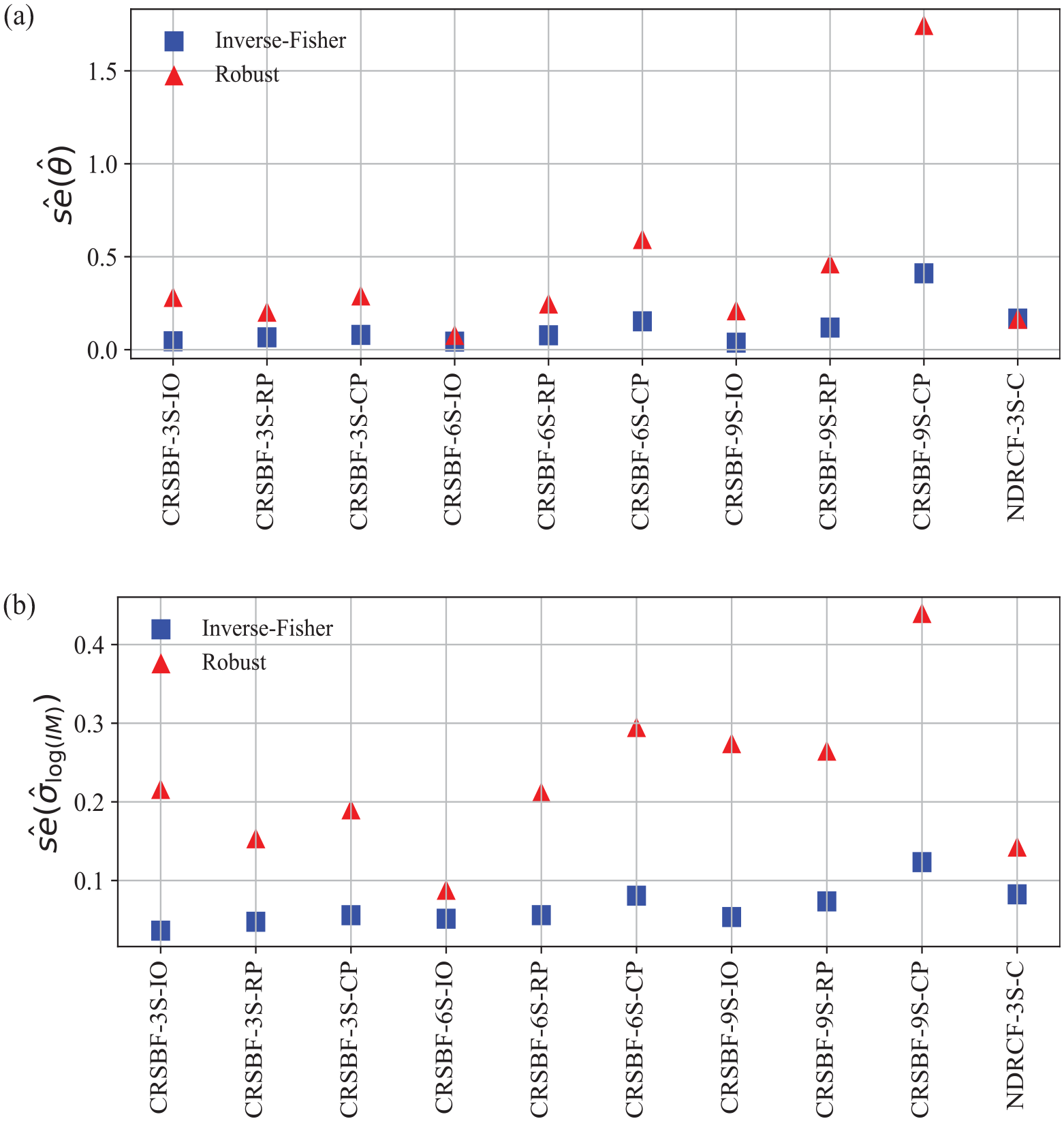
To provide some intuition regarding the differences between the two distinct standard errors, Figure 1 depicts the estimated standard errors for the two parameters in a lognormally specified fragility curve—the median of intensity measure $\left(\mathrm{IM}\right)$ , $\theta$ , and dispersion (or, log-standard deviation), ${\sigma }_{\log (\mathrm{IM})}$ , based on structural response data from previously published articles (Dastmalchi and Burton, 2021; Haindl et al., 2023). The data contain counts of building structures exceeding different limit states subjected to earthquake ground motion excitations at different intensity levels. The observation that the robust standard errors deviate from their IF-based counterparts signifies that the specification of the lognormal form is incorrect. This means that a greater number of ground motions is needed to achieve the precision that is obtained from the IF-based method. Later we introduce a method to detect misspecification through hypothesis testing.

Figure 1.

$\hat{s}e$ for (a) $\hat{m}$ and (b) ${\hat{\sigma }}_{\log (\mathrm{IM})}$ calculated from two types of standard errors based on data from the literature.

Simulation-based investigation

To demonstrate the superiority of the robust standard error over the classical standard error and reason intuitively about their differences, we create two hypothetical model misspecification scenarios that may arise in seismic assessments: misspecifying the link function and violating the independence assumption.

Generalized linear models (GLMs), which are often used for fragility fitting, are comprised of two components: the response variable $Y$ , which is a member of the exponential family, and a link function $q(·)$ that relates the conditional expectation of the response variable to the linear combination of predictors. In the case of a limit state fragility, the response variable is a dichotomous number, and only one predictor (i.e. $\mathrm{IM}$ ) exists. Therefore, the GLM has the form:

$$q(\mathbb{E}(Y|\mathrm{IM}))=q(P(Y=1|\mathrm{IM}))={\beta }_0+{\beta }_1\mathrm{IM},$$

(4)

where $P(Y=1|\mathrm{IM}):=p_{\mathrm{IM}}$ denotes the probability of attaining or exceeding some predefined limit state under a specified $\mathrm{IM}$ level.

If the probit link function is used (i.e. $q(·)={\Phi }^{-1}(·)$ where $\Phi$ is the standard normal cumulative density function (CDF)), and the predictor $\mathrm{IM}$ is replaced by its logarithmic form, $\log (\mathrm{IM})$ , then fitting the fragility based on the GLM is mathematically equivalent to using a lognormal CDF (e.g. Baker, 2015):

$$p_{\mathrm{IM}}=\Phi ({\beta }_0+{\beta }_1\log \mathrm{IM})=\Phi \left(\frac{\log (\mathrm{IM}/m)}{\sigma }\right),$$

(5)

The relationship between fragility parameters and GLM coefficients is as follows: $m=\exp \left(\frac{-{\beta }_0}{{\beta }_1}\right)$ is the median, and ${\sigma }_{\log (\mathrm{IM})}=\frac{1}{{\beta }_1}$ is the dispersion. With these relationships, the uncertainty in the GLM coefficients ${\beta }_0$ and ${\beta }_1$ can be transformed to that of the lognormal fragility parameters $m$ and ${\sigma }_{\log (\mathrm{IM})}$ .

Scenario 1: Misspecified link function

This subsection discusses the case where the specified probit link in a GLM deviates from the true link function that generates the data. Procedures for this simulation-based investigation are summarized below:

1. Specify the true GLM coefficients ${\beta }_0^{*}$ and ${\beta }_1^{*}$ in Equation 4.

2. Specify a true link function $q^{*}(·)$ (other than the probit link) from which the probability of limit state exceedance is generated: $p_{\mathrm{IM}}^{*}=q^{*-1}({\beta }_0^{*}+{\beta }_1^{*}\log \mathrm{IM})$ .

3. for $b=1:B$ (where $B$ is the total number of simulations) do

4.   (b) Use the misspecified probit link function to fit the GLM, and obtain ${\hat{\beta }}_0^b$ and ${\hat{\beta }}_1^b$ .

5.   (c) Estimate the standard errors of ${\hat{\beta }}_0^b$ and ${\hat{\beta }}_1^b$ using the two distinct methods, which are denoted as $\hat{s}{e}^{\mathrm{IF}}({\hat{\beta }}^b)$ and $\hat{s}{e}^{\mathrm{RB}}({\hat{\beta }}^b)$ , respectively.

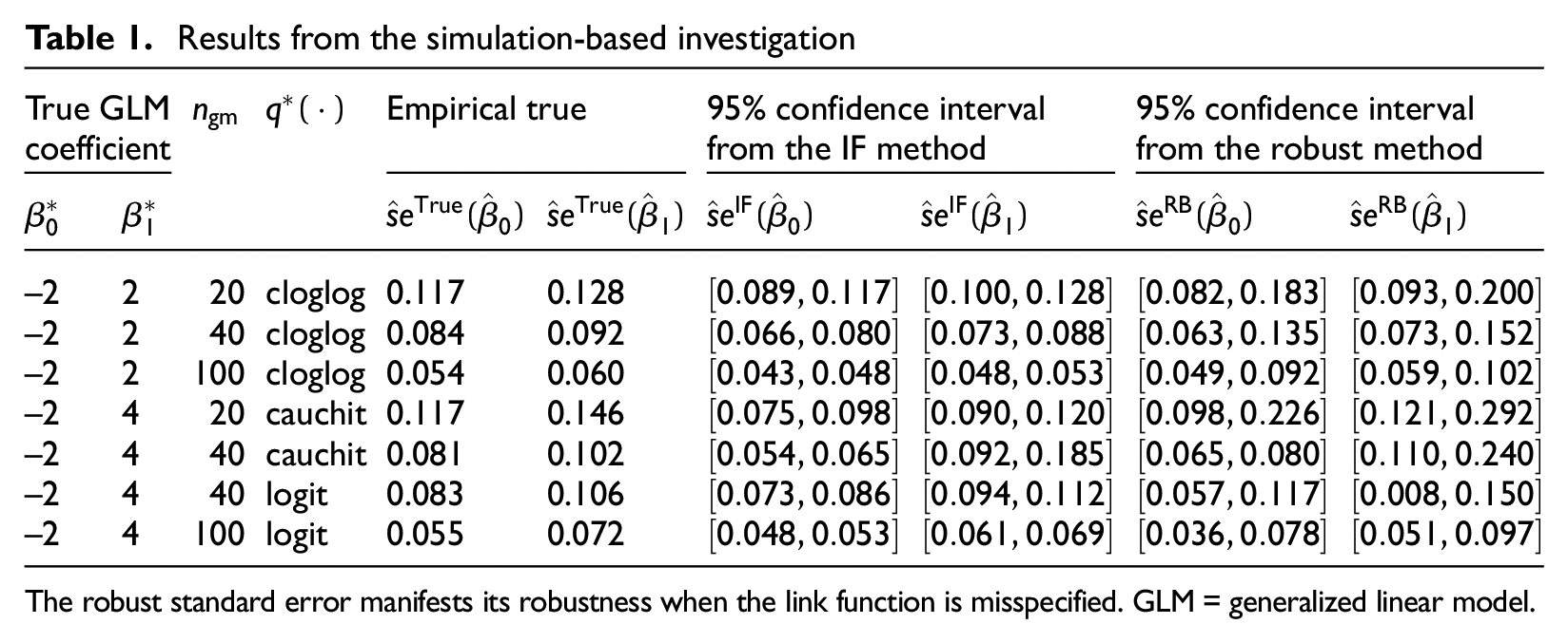
Now we have a set of $B$ -simulated GLM coefficients, ${\hat{\beta }}^b(b=1,\dots ,B)$ . The sample standard deviation from the simulated GLM coefficients is denoted as the empirical true standard error, $\hat{s}{e}^{\mathrm{True}}(\hat{\beta })$ .

Construct 95% confidence intervals from the sampling distributions of $\hat{s}{e}^{\mathrm{IF}}({\hat{\beta }}^b)$ and $\hat{s}{e}^{\mathrm{RB}}({\hat{\beta }}^b),\mathrm{where}(b=1,\dots ,B)$ .

The goal is to compare the 95% confidence intervals from the two types of standard errors and the empirical true value to demonstrate the superiority of the robust standard error. A total of $B=500$ simulations are performed. A fixed number of hypothetical ground motions is used at each IM level. The $\mathrm{IM}$ levels are defined from 0.1 to 4 with an increment of 0.1 (the unit is not important here).

Table 1 shows the result of this simulation study. The 95% confidence intervals from the robust standard errors (the last column) produce wider intervals than that of the IF-based method (the fifth column), and the former always contains the empirical true standard errors (the fourth column). In contrast, the confidence intervals from the IF-based method fail to capture the empirical true values. This indicates that the robust method is able to accurately estimate standard errors even when the probability model is misspecified.

Table 1.

Results from the simulation-based investigation

True GLM coefficient		$n_{\mathrm{gm}}$	$q^{*}(·)$	Empirical true		95% confidence interval from the IF method		95% confidence interval from the robust method
${\beta }_0^{*}$	${\beta }_1^{*}$			$\hat{s}{e}^{\mathrm{True}}({\hat{\beta }}_0)$	$\hat{s}{e}^{\mathrm{True}}({\hat{\beta }}_1)$	$\hat{s}{e}^{\mathrm{IF}}({\hat{\beta }}_0)$	$\hat{s}{e}^{\mathrm{IF}}({\hat{\beta }}_1)$	$\hat{s}{e}^{\mathrm{RB}}({\hat{\beta }}_0)$	$\hat{s}{e}^{\mathrm{RB}}({\hat{\beta }}_1)$
−2	2	20	cloglog	0.117	0.128	$[0.089,0.117]$	$[0.100,0.128]$	$[0.082,0.183]$	$[0.093,0.200]$
−2	2	40	cloglog	0.084	0.092	$[0.066,0.080]$	$[0.073,0.088]$	$[0.063,0.135]$	$[0.073,0.152]$
−2	2	100	cloglog	0.054	0.060	$[0.043,0.048]$	$[0.048,0.053]$	$[0.049,0.092]$	$[0.059,0.102]$
−2	4	20	cauchit	0.117	0.146	$[0.075,0.098]$	$[0.090,0.120]$	$[0.098,0.226]$	$[0.121,0.292]$
−2	4	40	cauchit	0.081	0.102	$[0.054,0.065]$	$[0.092,0.185]$	$[0.065,0.080]$	$[0.110,0.240]$
−2	4	40	logit	0.083	0.106	$[0.073,0.086]$	$[0.094,0.112]$	$[0.057,0.117]$	$[0.008,0.150]$
−2	4	100	logit	0.055	0.072	$[0.048,0.053]$	$[0.061,0.069]$	$[0.036,0.078]$	$[0.051,0.097]$

The robust standard error manifests its robustness when the link function is misspecified. GLM = generalized linear model.

Scenario 2: Violation of the independent observation assumption

An important assumption that is embedded in binomial random variables is that the individual trial observations are independent. This is also the assumption adopted in seismic fragility fitting procedures, that is, each observation of structural failure or not is assumed to be independent of all the others. However, this assumption may not be valid in many cases. For example, ground motions that are selected from the same earthquake event may cause dependency in seismic responses. Also, research on ground motion rotation considers different incidence angles for a fixed record, which violates the independence assumption.

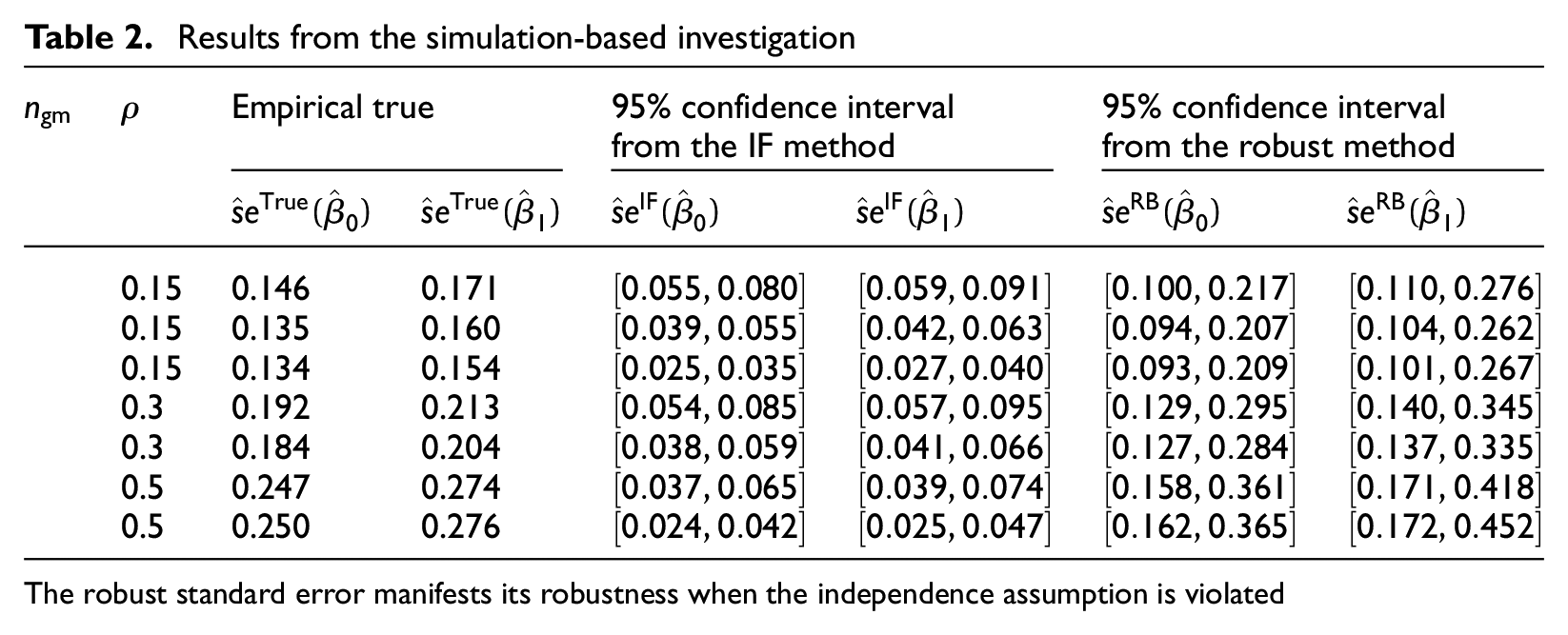
In this simulation setting, we draw dependent binomial numbers using the beta-binomial distribution (Wilcox, 1981), in which the probability of structural failure is dependent on a specific beta distribution:

$$P(Y=y\mathrm{out}\mathrm{of}n\mathrm{ground}\mathrm{motions}\mathrm{cause}\mathrm{failure}|\alpha ,\beta )=\left(\begin{array}{c}n\hfill \\ \multicolumn{1}{c}{y}\end{array}\right)\frac{B(y+\alpha ,n-y+\beta )}{B(\alpha ,\beta )},$$

(6)

which means the probability of observing $y$ failures out of $n$ ground motions is dependent on the beta distribution parameters $\alpha$ and $\beta$ . $B(·,·)$ is the beta function. A tuning parameter $\rho =\frac{1}{1+\alpha +\beta }\in [0,1)$ is used to control the degree of dependence. We use $\mathrm{IM}$ levels from 0.1 to 4 with an increment of 0.1. The true probability of failure at the $j\mathrm{th}$ $\mathrm{IM}$ level is assumed to be $0.1+0.8\times \frac{j}{40}(j=1,\dots ,40)$ . A total of 500 simulations are performed. The probit link is specified as the probability model. The results in Table 2 show similar trends as the preceding stimulation study. The confidence intervals from the robust approach always contain the empirical true standard errors, while the confidence intervals from the IF-based method do not. This demonstrates the superiority of $\hat{s}{e}^{\mathrm{RB}}$ in estimating the standard errors of GLM coefficients when the independence assumption is violated.

Table 2.

Results from the simulation-based investigation

$n_{\mathrm{gm}}$	$\rho$	Empirical true		95% confidence interval from the IF method		95% confidence interval from the robust method
		$\hat{s}{e}^{\mathrm{True}}({\hat{\beta }}_0)$	$\hat{s}{e}^{\mathrm{True}}({\hat{\beta }}_1)$	$\hat{s}{e}^{\mathrm{IF}}({\hat{\beta }}_0)$	$\hat{s}{e}^{\mathrm{IF}}({\hat{\beta }}_1)$	$\hat{s}{e}^{\mathrm{RB}}({\hat{\beta }}_0)$	$\hat{s}{e}^{\mathrm{RB}}({\hat{\beta }}_1)$
	0.15	0.146	0.171	$[0.055,0.080]$	$[0.059,0.091]$	$[0.100,0.217]$	$[0.110,0.276]$
	0.15	0.135	0.160	$[0.039,0.055]$	$[0.042,0.063]$	$[0.094,0.207]$	$[0.104,0.262]$
	0.15	0.134	0.154	$[0.025,0.035]$	$[0.027,0.040]$	$[0.093,0.209]$	$[0.101,0.267]$
	0.3	0.192	0.213	$[0.054,0.085]$	$[0.057,0.095]$	$[0.129,0.295]$	$[0.140,0.345]$
	0.3	0.184	0.204	$[0.038,0.059]$	$[0.041,0.066]$	$[0.127,0.284]$	$[0.137,0.335]$
	0.5	0.247	0.274	$[0.037,0.065]$	$[0.039,0.074]$	$[0.158,0.361]$	$[0.171,0.418]$
	0.5	0.250	0.276	$[0.024,0.042]$	$[0.025,0.047]$	$[0.162,0.365]$	$[0.172,0.452]$

The robust standard error manifests its robustness when the independence assumption is violated

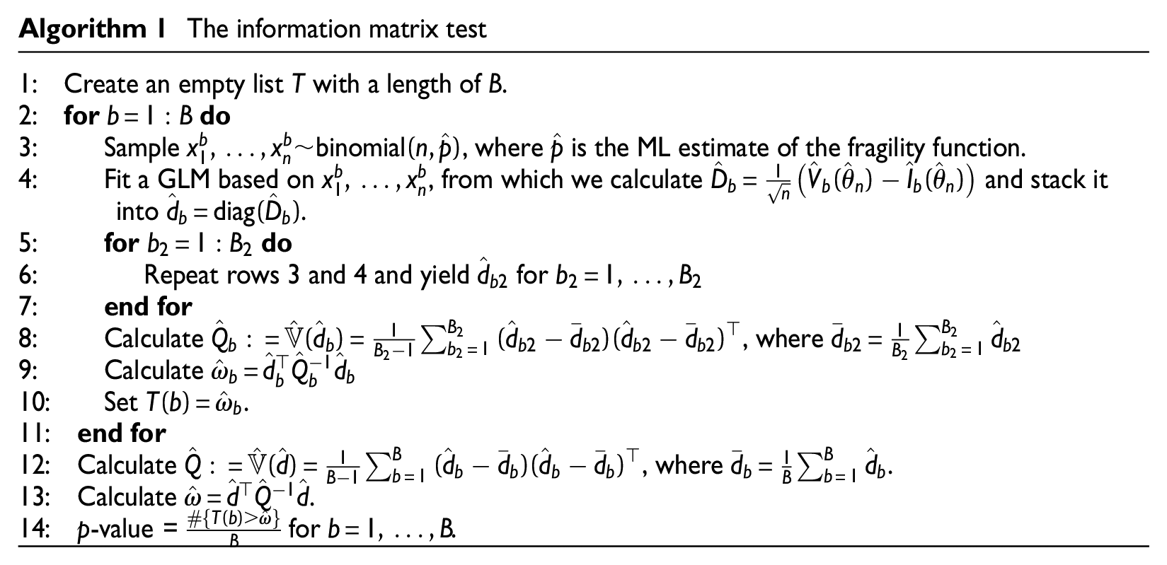
The information matrix test

Several methods exist for diagnosing probability model specification. For instance, the quantile–quantile plot allows for visual comparisons of the data against the presumed distribution (e.g. Jayaram and Baker, 2008). On the other hand, hypothesis testing can be employed if the data conforms to the presumed distribution.

In this article, we use the information matrix test (a variant of hypothesis testing) initially introduced by White (1982) to detect misspecification. By comparing Equations 1 and 2, misspecification exists if the meat matrix (the middle matrix in the robust standard error) diverges from the observed information matrix. This leads to the null and alternative hypotheses:

$$H_0:(V({\hat{\theta }}_n){)}_{\mathrm{kl}}=(I({\hat{\theta }}_n){)}_{\mathrm{kl}}$$

(7a)

$$H_a:(V({\hat{\theta }}_n){)}_{\mathrm{kl}}\ne (I({\hat{\theta }}_n){)}_{\mathrm{kl}},\mathrm{for}1\le k,l\le p$$

(7b)

The information matrix test identifies whether there exists a statistically significant divergence between the two matrices. The method proposed in Dhaene and Hoorelbeke (2004) is adopted, which used a nested parametric bootstrap to calculate the $p$ -value of the information matrix test.

To derive the test statistic, first, for $\hat{V}({\hat{\theta }}_n)$ and $\hat{I}({\hat{\theta }}_n)$ obtained from $x_1,\dots ,x_n$ which are binary numbers corresponding to the exceedance of a certain limit state or not, we calculate $\hat{D}=\frac{1}{\sqrt{n}}(\hat{V}({\hat{\theta }}_n)-\hat{I}({\hat{\theta }}_n))$ . The matrix is then stacked into a vector of length $p$ : $\hat{d}=\mathrm{diag}(\hat{D})$ . The test statistic is expressed as $\hat{\omega }={\hat{d}}^{\top }{\hat{Q}}^{-1}\hat{d}$ , where $\hat{Q}$ is the consistent estimate of $\hat{\mathbb{V}}(\hat{d})$ under $H_0$ . To estimate $\hat{Q}$ and the subsequent $p$ -value, we adopt the nested bootstrap in Dhaene and Hoorelbeke (2004), which is summarized below:

Algorithm 1

The information matrix test

1: Create an empty list $T$ with a length of $B$ .2: for $b=1:B$ do3:   Sample $x_1^b,\dots ,x_n^b~\mathrm{binomial}(n,\hat{p})$ , where $\hat{p}$ is the ML estimate of the fragility function.4:   Fit a GLM based on $x_1^b,\dots ,x_n^b$ , from which we calculate ${\hat{D}}_b=\frac{1}{\sqrt{n}}({\hat{V}}_b({\hat{\theta }}_n)-{\hat{I}}_b({\hat{\theta }}_n))$ and stack it into ${\hat{d}}_b=\mathrm{diag}({\hat{D}}_b)$ .5:   for $b_2=1:B_2$ do6:     Repeat rows 3 and 4 and yield ${\hat{d}}_{b2}$ for $b_2=1,\dots ,B_2$ 7:   end for8:   Calculate ${\hat{Q}}_b:=\hat{\mathbb{V}}({\hat{d}}_b)=\frac{1}{B_2-1}\sum _{b_2=1}^{B_2}({\hat{d}}_{b2}-{\overline{d}}_{b2})({\hat{d}}_{b2}-{\overline{d}}_{b2}{)}^{\top }$ , where ${\overline{d}}_{b2}=\frac{1}{B_2}\sum _{b_2=1}^{B_2}{\hat{d}}_{b2}$ 9:   Calculate ${\hat{\omega }}_b={\hat{d}}_b^{\top }{\hat{Q}}_b^{-1}{\hat{d}}_b$ 10:  Set $T(b)={\hat{\omega }}_b$ .11: end for12: Calculate $\hat{Q}:=\hat{\mathbb{V}}(\hat{d})=\frac{1}{B-1}\sum _{b=1}^B({\hat{d}}_b-{\overline{d}}_b)({\hat{d}}_b-{\overline{d}}_b{)}^{\top }$ , where ${\overline{d}}_b=\frac{1}{B}\sum _{b=1}^B{\hat{d}}_b$ .13: Calculate $\hat{\omega }={\hat{d}}^{\top }{\hat{Q}}^{-1}\hat{d}$ .14:  $p$ -value =  $\frac{\#\{T(b)>\hat{\omega }\}}{B}$ for $b=1,\dots ,B$ .

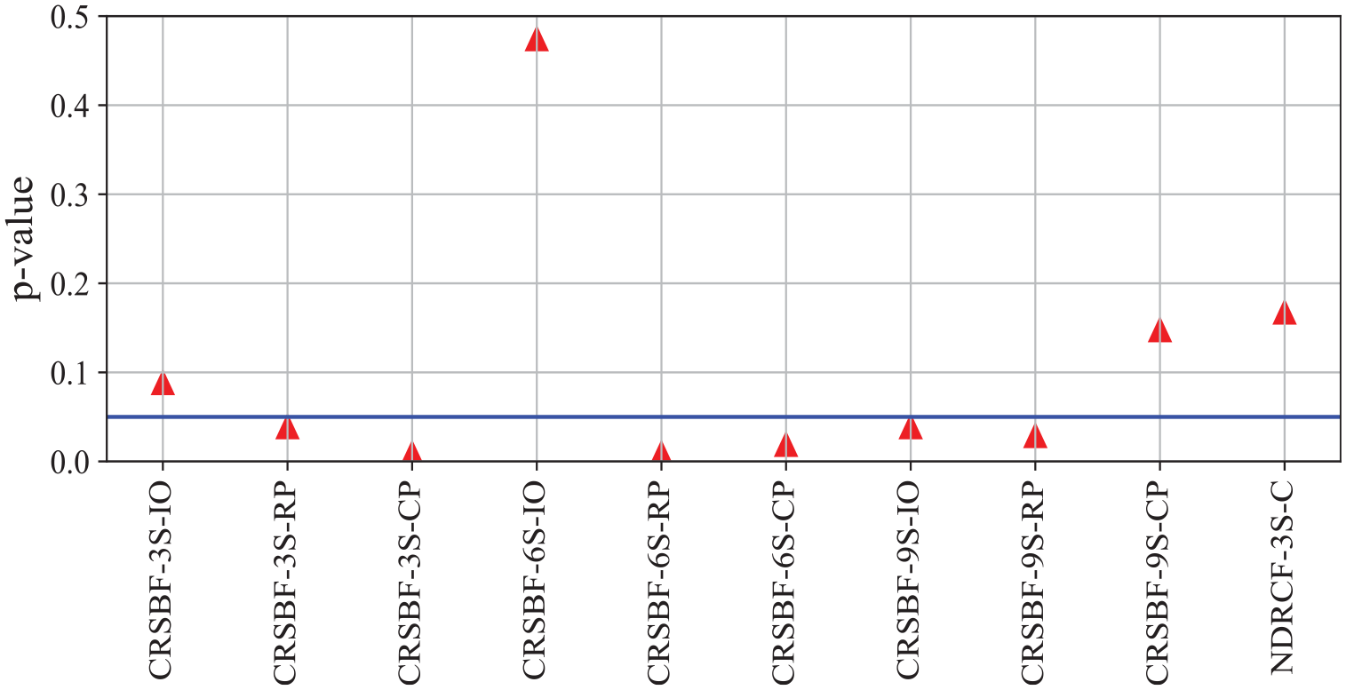
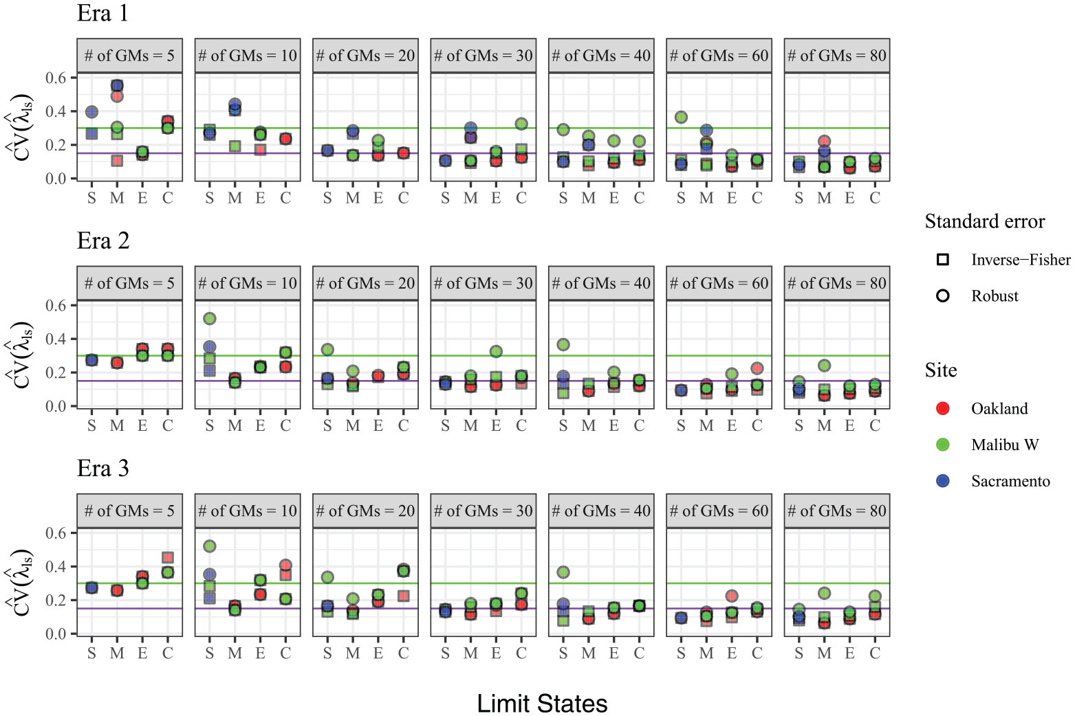
Figure 2 shows the $p$ -values of the information matrix test for the same data used in Figure 1. By specifying a significance level of 0.05, the $H_0$ is rejected in six out of ten cases which implies misspecification.

Figure 2.

p-Values from the information matrix test based on data from the literature.

Description of bridges, structural modeling, and performance limit states

The effects of misspecification are investigated with respect to probabilistic seismic responses and risk analyses of California bridges. The goal is to uncover how the adoption of the robust standard error influences the estimation uncertainty in the seismic response and risk.

Description of bridges and nonlinear structural modeling

Two-span box girders are one of the most commonly used bridge superstructures in the state of California. As such, two-span seat-type bridges with a single column designed in different eras are used as the case study structures.

The bridge nonlinear structural modeling strategy in Mangalathu (2017) is adopted. Three-dimensional bridge models are constructed and analyzed using OpenSeesPy (Zhu et al., 2018).

The bridge superstructure comprises elasticBeamColumn elements with concentrated masses along the centerline, assuming the superstructure maintains elasticity during an earthquake. The transverse connection between the bridge deck and the abutment is modeled using a rigidLink element. The column bents are modeled using dispBeamColumn elements with four integration points. The sections are discretized into steel (Steel02), and unconfined and confined concrete (Concrete07) fibers.

Translational and rotational linear springs are added at the column base to represent the foundation–soil interaction. The response of the abutment in the longitudinal direction is governed by passive and active resistance. Passive resistance is developed in parallel by the backfill soil and abutment piles when the abutment backwall moves toward the backfill soil. Active resistance is developed when the abutment moves away from the backfill soil and is influenced by the abutment piles only. The abutment transverse response is resisted by the piles only. The backfill soil is modeled using zero-length elements in the longitudinal direction, with the HyperbolicGap material. The pile behaviors in the longitudinal and transverse directions are modeled using bi-directional zero-length elements, with the hysteretic material.

The expansion joint between the deck and abutment consists of three components: the elastomeric bearings, pounding between the deck and abutment, and shear keys. The bi-directional behavior of the bearings is simulated via the Steel01 material. The shear key in the transverse direction is modeled using the trilinear material with a gap. The pounding in the longitudinal direction is modeled using the ElasticPPGap material.

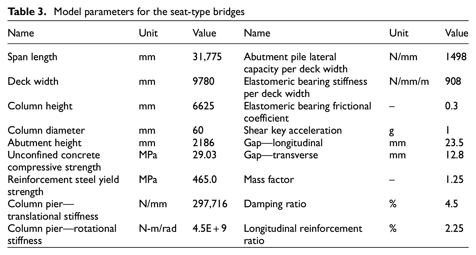
Model parameter uncertainty is not considered. Therefore, the associated parameters are taken as their expected (for normal distributed variables) or median values (for lognormal distributed variables) based on the probability models defined in Mangalathu (2017). A mass factor, serving as a multiplier applied to the original mass, accounts for the fact that superstructure components, such as parapets and rails, are not explicitly considered in the bridge model. The same geometry (including the span length, deck width, column height, etc.) is used for bridges designed in different eras. The bridge modeling parameters are summarized in Table 3. Readers can refer to Figure 3.2 in Mangalathu (2017) for the bridge model schematic.

Table 3.

Model parameters for the seat-type bridges

Name	Unit	Value	Name	Unit	Value
Span length	mm	31,775	Abutment pile lateral capacity per deck width	N/mm	1498
Deck width	mm	9780	Elastomeric bearing stiffness per deck width	N/mm/m	908
Column height	mm	6625	Elastomeric bearing frictional coefficient	–	0.3
Column diameter	mm	60	Shear key acceleration	g	1
Abutment height	mm	2186	Gap—longitudinal	mm	23.5
Unconfined concrete compressive strength	MPa	29.03	Gap—transverse	mm	12.8
Reinforcement steel yield strength	MPa	465.0	Mass factor	–	1.25
Column pier—translational stiffness	N/mm	297,716	Damping ratio	%	4.5
Column pier—rotational stiffness	N-m/rad	4.5E+9	Longitudinal reinforcement ratio	%	2.25

Bridge performance limit states

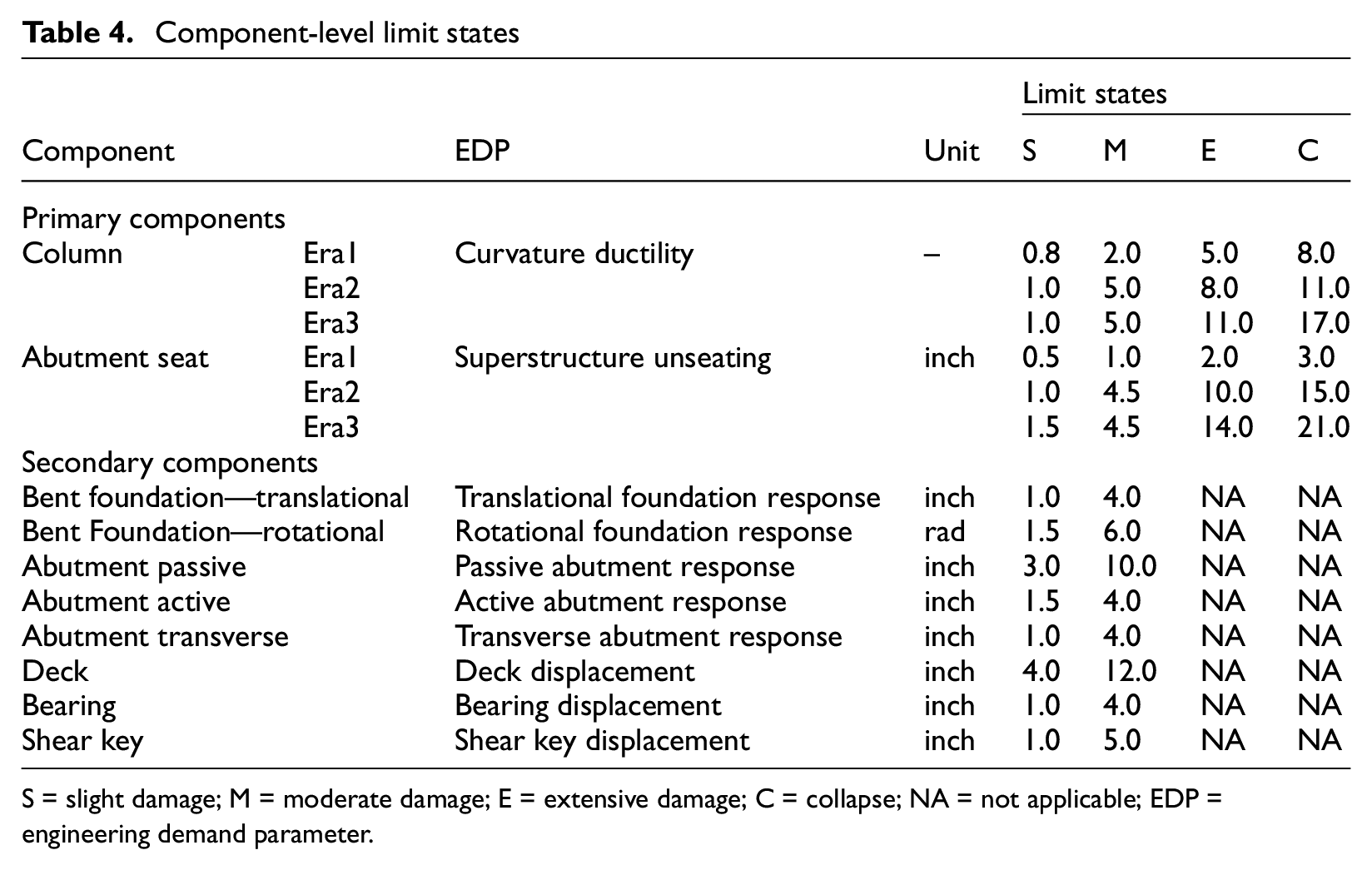
Three bridge design eras are considered, including pre-1971 (Era1), 1971–1990 (Era2), and post-1990 (Era3). The differences among the design eras are reflected in the component and system seismic capacities. Bridge components are categorized into primary or secondary. Primary components include the columns and abutment seats, which affect bridge safety. Secondary components include the abutment piles and backfill soil, expansion joints, and decks, whose failure affects serviceability but does not compromise safety. The bridge is treated as a multicomponent system, where system failure is determined by the failure of its ten constituent components. A series system is assumed where the exceedance counts for the bridge are calculated as the envelope of the component exceedance counts (Li et al., 2020). The component-level limit states for bridges designed in three eras are shown in Table 4 (Mangalathu, 2017).

Table 4.

Component-level limit states

				Limit states
Component		EDP	Unit	S	M	E	C
Primary components
Column	Era1	Curvature ductility	–	0.8	2.0	5.0	8.0
	Era2			1.0	5.0	8.0	11.0
	Era3			1.0	5.0	11.0	17.0
Abutment seat	Era1Era2Era3	Superstructure unseating	inch	0.51.01.5	1.04.54.5	2.010.014.0	3.015.021.0
Secondary components
Bent foundation—translational		Translational foundation response	inch	1.0	4.0	NA	NA
Bent Foundation—rotational		Rotational foundation response	rad	1.5	6.0	NA	NA
Abutment passive		Passive abutment response	inch	3.0	10.0	NA	NA
Abutment active		Active abutment response	inch	1.5	4.0	NA	NA
Abutment transverse		Transverse abutment response	inch	1.0	4.0	NA	NA
Deck		Deck displacement	inch	4.0	12.0	NA	NA
Bearing		Bearing displacement	inch	1.0	4.0	NA	NA
Shear key		Shear key displacement	inch	1.0	5.0	NA	NA

S = slight damage; M = moderate damage; E = extensive damage; C = collapse; NA = not applicable; EDP = engineering demand parameter.

Hazard characterization

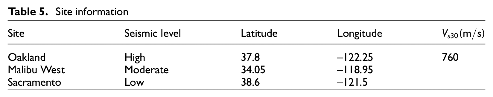
Probabilistic seismic hazard analysis (PSHA) is performed at the sites of interest. Varying levels of seismic hazard are considered by selecting three sites in California located in Oakland (high seismicity), Malibu West (moderate seismicity), and Sacramento (low seismicity). The time averaged shear-wave velocity for the upper 30-m depth $\left(V_{s30}\right)$ is taken as $760\mathrm{m}/\mathrm{s}$ , assuming all the sites are in NEHRP soil class BC (Building Seismic Safety Council, 2003; i.e. $660\mathrm{m}/\mathrm{s}<V_{s30}<945\mathrm{m}/\mathrm{s}$ ). The seismicity-level descriptors for these three sites are defined relative to other cities in California. The site information is shown in Table 5. The three coordinates are based on the US Geological Survey (USGS) reference locations (Petersen et al., 2015).

Table 5.

Site information

Site	Seismic level	Latitude	Longitude	$V_{s30}(\mathrm{m}/\mathrm{s})$
Oakland	High	37.8	−122.25	760
Malibu West	Moderate	34.05	−118.95
Sacramento	Low	38.6	−121.5

The geometric mean spectral acceleration over a range of periods, $S{a}_{\mathrm{avg}}:={(\sum _{i=1}^{N_T}\mathrm{Sa}(T_i))}^{\frac{1}{N_T}}$ (where $\mathrm{Sa}(T_i)$ is the spectral acceleration at period $T_i$ and $N_T$ is the number of structural periods chosen) is utilized as the $\mathrm{IM}$ . This $\mathrm{IM}$ is chosen because a bridge is typically dominated by more than one mode of vibration. $S{a}_{\mathrm{avg}}$ has been shown to be a more efficient $\mathrm{IM}$ for probabilistic seismic demand and performance assessment for structures affected by higher mode response (Cordova et al., 2000; Eads et al., 2013; Vamvatsikos and Cornell, 2005). The first six model periods are as follows: $T_{1x}=0.67\mathrm{s}$ (longitudinal), $T_{1y}=0.61\mathrm{s}$ (transverse), $T_{1z}=0.32\mathrm{s}$ (torsion), $T_{2x}=0.27\mathrm{s}$ (longitudinal), $T_{3x}=0.20\mathrm{s}$ (longitudinal), and $T_{2y}=0.09\mathrm{s}$ (transverse). $S{a}_{\mathrm{avg}}$ is computed as the geometric mean from $T_{2y}=0.1\mathrm{s}$ to $1.5T_{1x}=1.0\mathrm{s}$ with a uniform period spacing of $0.10\mathrm{s}$ .

PSHA is performed using the OpenQuake Hazard Characterization engine (Pagani et al., 2014). We use the UCERF3 model (Field et al., 2014) to characterize rupture rates for the seismic sources in California. The GMM proposed by Boore et al. (2014) is specified to predict the seismic intensity in active shallow crustal tectonic zones. The constituent $\mathrm{Sa}(T_i)s$ in $S{a}_{\mathrm{avg}}$ is developed based on 5%-damped orientation-independent spectral coordinate, $\mathrm{RotD}50$ (Boore, 2010), where the directionality of the two orthogonal horizontal ground motion pairs is considered. The subsequent ground motion selection and scaling schemes are also based on $S{a}_{\mathrm{avg},\mathrm{RotD}50}$ , but we omit the $\mathrm{RotD}50$ subscript for simplicity. The correlation model for $\mathrm{Sa}$ at different periods developed by Baker and Jayaram (2008) is used to quantify the dependence for the $S{a}_{\mathrm{avg}}$ calculation.

Six $\mathrm{IM}$ levels with return periods of 50, 225, 475, 975, 2475, and 10,000 years are considered in the risk-based assessment. The 225- and 975-year return periods correspond to, respectively, the functional and safety-evaluation earthquakes in the Caltrans SDC v2.0 (California Department of Transportation, 2018). The 475- and 2475-year return periods are defined as the design-basis and maximum-considered earthquakes, respectively, in ASCE 7-22 (American Society of Civil Engineers, 2022).

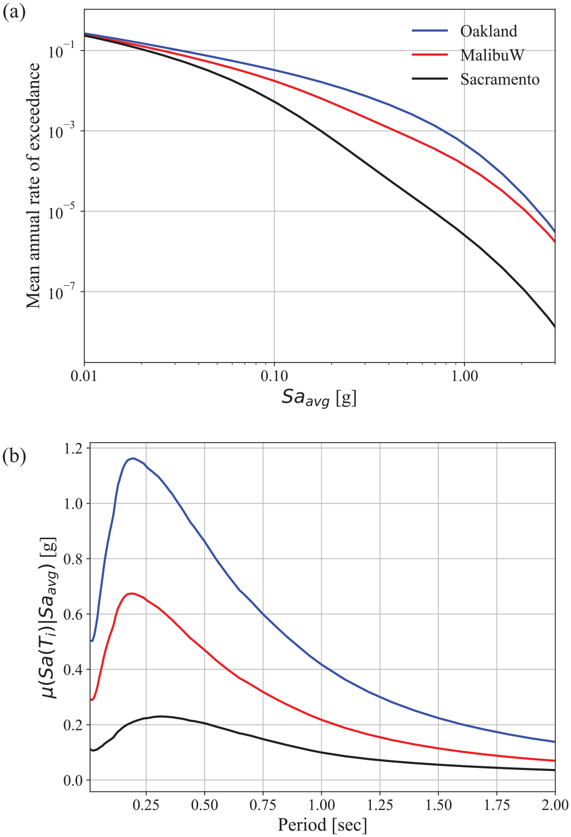
The hazard curves and conditional mean spectra (CMSs; Baker, 2011) for the three sites are shown in Figure 3. The CMS is approximated based on the results of mean hazard disaggregation. It is apparent that Oakland has the highest seismicity, while Sacramento has the lowest.

Figure 3.

(a) Hazard curves and (b) $\mathrm{CMS}(\mathrm{Sa}(T_i)|S{a}_{\mathrm{avg}})$ at a return period of 975 years, for the three sites.

Quantifying the effects of model misspecification on the required number of ground motions

Seismic analysis procedures for parametric probability models involve: (1) selecting a finite number of ground motions that represent the site hazard, (2) performing nonlinear response history analyses (NRHAs) based on the selected ground motions, (3) fitting a probability model based on the structural response data, and (4) making statistical inferences about the parameters that define the probability model. Due to the finite sample size, using different sets of ground motions yields different parameter estimates. The variability in the parameter estimates is described as the estimation uncertainty.

This section investigates the effects of the number of ground motions on parameter estimation uncertainty, both in code-prescriptive and risk-based assessments. Misspecification potential and its impact on estimation uncertainty and the required number of ground motions are also explicitly considered. Different inferential statistics are used for the two seismic evaluation procedures. The code-based assessment focuses on the precision of the descriptive statistics (e.g. mean, median, and standard deviation) for the EDPs of interest, while the risk-based assessment considers the precision of the mean annual frequency of exceeding different performance limit states. Specifically, the $\mathrm{CV}$ of the median and dispersion estimates of a critical bridge EDP are considered for the code-based assessment. In the risk-based assessment, we use the $\mathrm{CV}$ of the mean annual frequency of exceeding the slight, moderate, extensive, and collapse limit states.

Since most prior research and applications related to probabilistic seismic performance assessments specify the lognormal distribution as the functional form, we stick to using this probability model in both the code-prescriptive and risk-based procedures.

Code-prescriptive assessment

A code-prescriptive assessment in which NRHA is performed at a single or multiple $\mathrm{IM}$ levels is commonly adopted in seismic design procedures (Baker et al., 2021: Chapter 10). The goal of this type of assessment is to estimate the parameters that define the conditional (on the $\mathrm{IM}$ ) probability distributions of the critical EDPs and ensure that the summary statistic (e.g. the mean) is below some predefined threshold. A minimum number of ground motions that must be selected based on a target spectrum is typically specified in seismic codes, standards, and guidelines. This minimum number is specified under the assumption that it will yield reliable estimates from the resulting sample.

The model for a specific EDP that expresses the probability of exceeding certain values conditional on an $\mathrm{IM}$ is given by:

$$P(\mathrm{EDP}>\mathrm{edp}|\mathrm{IM})=1-\Phi \left(\frac{\log (\mathrm{edp}/m_{\mathrm{EDP}|\mathrm{IM}})}{{\sigma }_{\log (\mathrm{EDP})|\mathrm{IM}}}\right),$$

(8)

where $m_{\mathrm{EDP}|\mathrm{IM}}$ and ${\sigma }_{\log (\mathrm{EDP})|\mathrm{IM}}$ are the conditional median and dispersion for the EDP of interest. We are interested in the uncertainty in the maximum likelihood estimates for these two parameters because they control the required number of ground motions.

The relationship between the estimation uncertainty of the maximum curvature ductility $\left({\varphi }_m\right)$ of bridge columns and the number of ground motions is established. The Caltrans SDC v2.0 design spectrum is chosen as the target. The same document specifies the uniform hazard spectrum (UHS) at a return period of 975 years as the design spectrum. It is based on the 2014 version of the USGS seismic hazard map (Petersen et al., 2015), and adjusts for the UHS by incorporating amplification factors to account for near-fault and basin effects.

We choose ${\varphi }_m$ as the EDP of interest because it is often used as a measure of bridge safety and overall performance (e.g. Kowalsky et al., 1995; Zahn et al., 1986). ${\varphi }_m$ is the ratio between the maximum absolute curvature and the column yield curvature, ${\varphi }_y$ . The latter is obtained from a column section analysis as $3.66\times {10}^{-5}\mathrm{rad}$ .

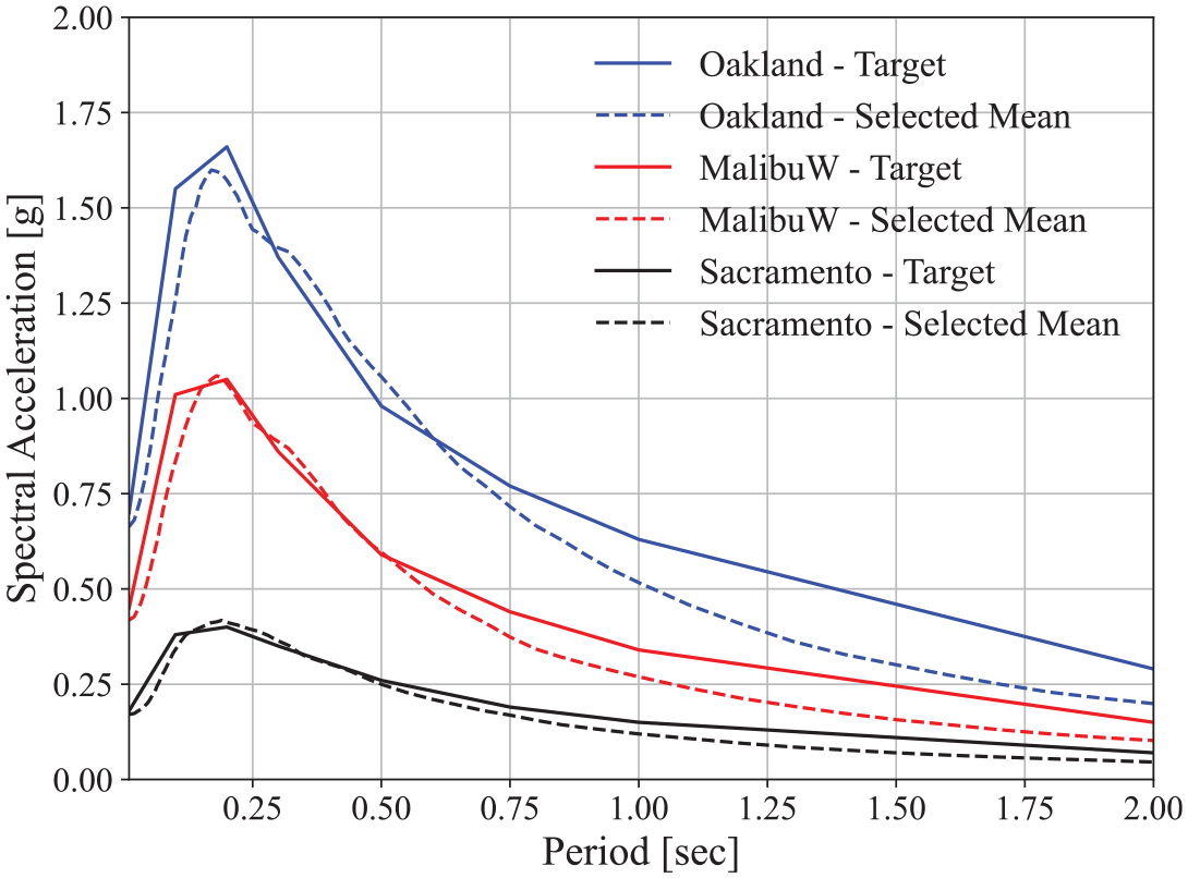
To investigate the impact of the number of ground motions on the estimation uncertainty of ${\varphi }_m$ , we vary $n_{\mathrm{gm}}$ from 3 to 200. For each $n_{\mathrm{gm}}$ , we calculate the $\mathrm{CV}$ of ${\hat{m}}_{{\varphi }_m|\mathrm{IM}}$ and ${\hat{\sigma }}_{\log ({\varphi }_m|\mathrm{IM})}$ . One strategy is to repeatably select ground motions that are consistent with the design spectrum, perform NRHA, and estimate the inferential statistics, from $n_{\mathrm{gm}}=\{3,\dots ,200\}$ . Recall the Caltrans design spectrum is a single mean spectrum, such that the candidate ground motions are selected based on a ranking of their individual mean-squared errors (MSEs). Therefore, we use the following approach: first, 200 ground motions are selected from the PEER NGA-West2 database (Bozorgnia et al., 2014) to match the design spectrum. Then, the records with the $n_{\mathrm{gm}}$ lowest MSE in the 200 ground motion set are chosen. The median and dispersion estimates for ${\varphi }_m$ as well as their estimation uncertainty are obtained based on the $n_{\mathrm{gm}}$ subset. Figure 4 shows the Caltrans design spectra, as well as the mean spectra of the selected 200 ground motions, for each of the three sites.

Figure 4.

Selected ground motions that match the Caltrans Seismic Design Criterion v2.0 design spectrum.

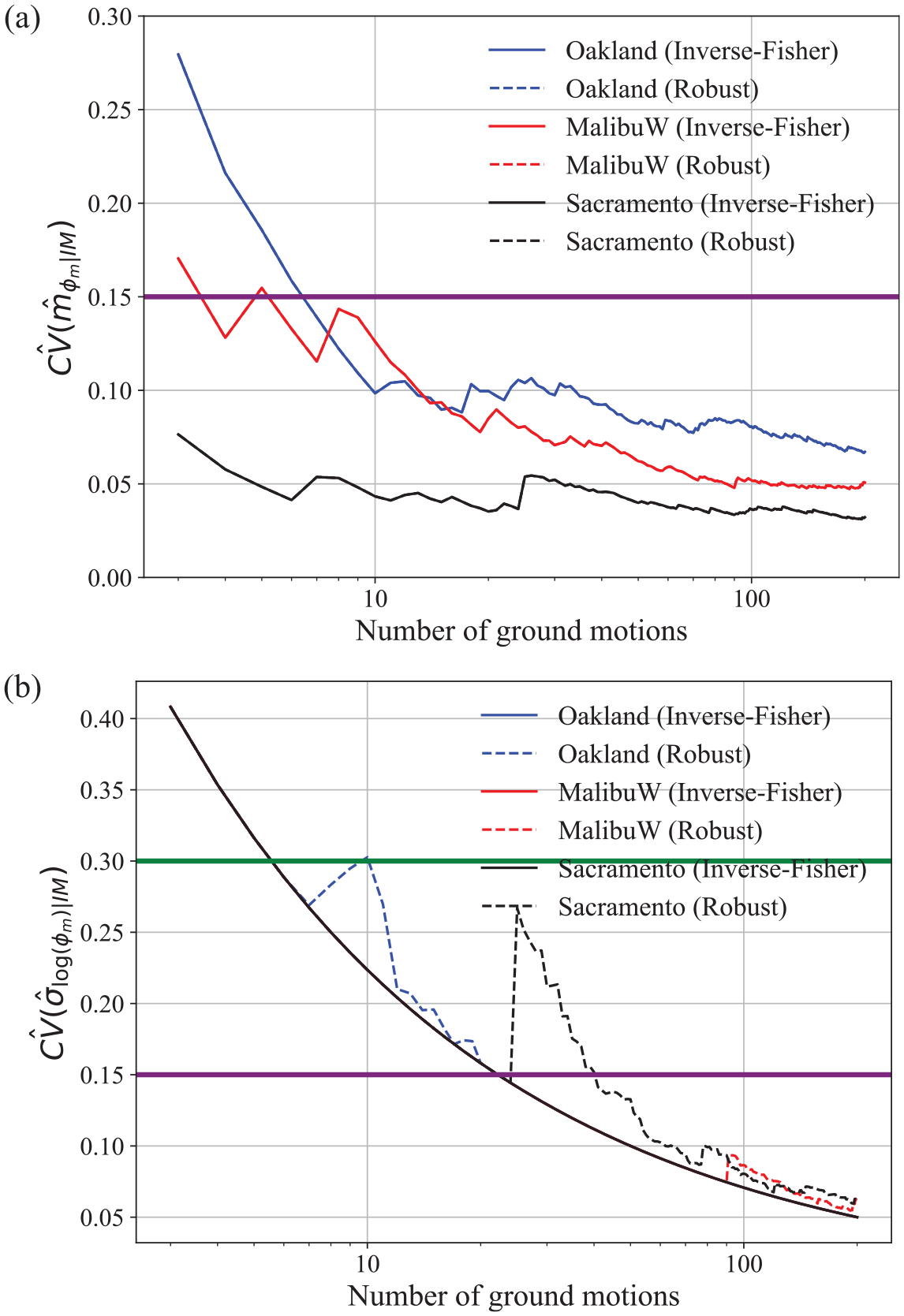
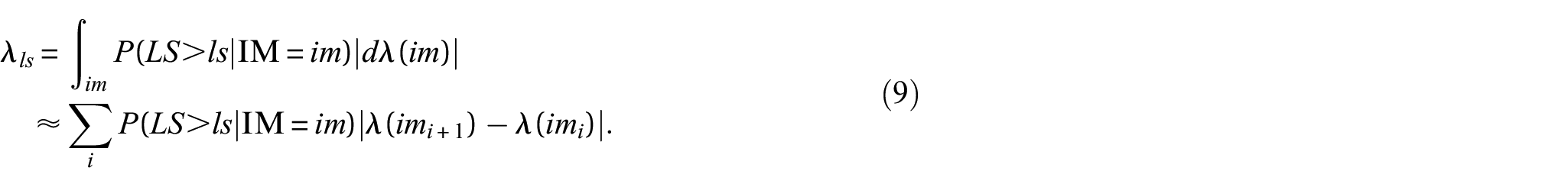
Figure 5 shows the $\mathrm{CV}$ estimates from the IF-based and robust methods for ${\hat{m}}_{{\varphi }_m|\mathrm{IM}}$ and ${\hat{\sigma }}_{\log ({\varphi }_m)|\mathrm{IM}}$ for different sizes of record-sets used in the NRHAs. For comparison purposes, we specify two variability levels: a moderate variability level corresponding to a CV of 0.3, and a low variability level with a CV of 0.15. This setting is subjective and can be adjusted depending on specific engineering needs. As expected, the $\mathrm{CV}$ estimates in general decrease as $n_{\mathrm{gm}}$ increases; however, there are some fluctuations, especially when a small sample size is used. This is because the standard errors are derived in the asymptotic context. Although they are inversely proportional to $\sqrt{n_{\mathrm{gm}}}$ , their plug-in estimates do not guarantee a monotonically decreasing trend.

Figure 5.

(a) $\hat{C}V({\hat{m}}_{{\varphi }_m|\mathrm{IM}})$ and (b) $\hat{C}V(\hat{\sigma }{)}_{\log ({\varphi }_m)|\mathrm{IM}}$ versus the $n_{\mathrm{gm}}$ used in the design phase.

The $\mathrm{CV}$ estimates for ${\hat{m}}_{{\varphi }_m|\mathrm{IM}}$ decrease sharply from $n_{\mathrm{gm}}=3$ to $20$ , and converge gradually after $n_{\mathrm{gm}}=30$ , for all three sites. In general, there is no difference between the results from the IF-based and robust methods (notice that they overlap in Figure 5a). This means the specification of the lognormal functional form for the median estimation is essentially correct. Also, observe that the site with the highest seismicity (Oakland) exhibits the highest $\hat{\mathrm{C}}\mathrm{V}({\hat{m}}_{{\varphi }_m|\mathrm{IM}})$ , while the site with the lowest seismic activity (Sacramento) shows the lowest.

The $\mathrm{CV}$ estimates for ${\hat{\sigma }}_{\log ({\varphi }_m)|\mathrm{IM}}$ (Figure 5b) without considering model misspecification are the same for all three sites. Supplement B shows that, for any normally or lognormally distributed random variables, the $\mathrm{CV}$ estimate of dispersion is independent of specific sample values. This means that if the goal is to determine the minimum $n_{\mathrm{gm}}$ based on the estimation uncertainty of ${\sigma }_{\log ({\varphi }_m)|\mathrm{IM}}$ without considering the possibility of misspecification, this can be done without performing any upfront structural analysis. This finding is exclusive to $\hat{\mathrm{C}}{\mathrm{V}}^{\mathrm{IF}}\left({\hat{\sigma }}_{\log ({\varphi }_m)|\mathrm{IM}}\right)$ .

There is obvious evidence of misspecification when using the lognormal form to estimate the dispersion. For example, $\hat{\mathrm{C}}{\mathrm{V}}^{\mathrm{RB}}\left({\hat{\sigma }}_{\log ({\varphi }_m)|\mathrm{IM}}\right)$ is significantly larger than $\hat{\mathrm{C}}{\mathrm{V}}^{\mathrm{IF}}\left({\hat{\sigma }}_{\log ({\varphi }_m)|\mathrm{IM}}\right)$ when $n_{\mathrm{gm}}\in \{7,12\}$ for Oakland. Misspecification is more severe for Sacramento, which happens when $n_{\mathrm{gm}}>24$ . For Malibu West, model misspecification is milder compared to Oakland and Sacramento. However, there is evidence showing slight misspecification when $n_{\mathrm{gm}}\ge 90$ . The occurrence of model misspecification in dispersion estimation suggests that caution should be taken when using the analytical form in Supplement B, which is based on the correct specification assumption. The $n_{\mathrm{gm}}$ from the IF-based method is 22 if the goal is to have low variability in $\hat{\mathrm{C}}\mathrm{V}\left({\hat{\sigma }}_{\log ({\varphi }_m)|\mathrm{IM}}\right)$ for the Sacramento site. This number increases to 41 when the robust standard error is considered. Therefore, QMLE is recommended when the precision of the dispersion is of interest.

The Caltrans SDC v2.0 Section 4.2.3 requires at least 7 ground motions for NRHAs. In our example application, $n_{\mathrm{gm}}=7$ produces median estimates with a low variability level $(\mathrm{CV}\le 0.15)$ . This indicates that using 7 ground motions is sufficient to yield reliable estimates for the median EDP of the considered bridges. In addition, misspecification is identified in dispersion estimates at all sites across various ranges of record-set sizes, which is evidenced by the discrepancy between the two types of standard errors. This happens in the $n_{\mathrm{gm}}$ range of 8–16 for Oakland, 25–200 for Sacramento, and 91–200 for Malibu West. This is a sign of misspecification since deviance should not happen if the model is correctly specified.

Does the increased $\hat{\mathrm{C}}\mathrm{V}({\hat{\sigma }}_{\log ({\varphi }_m)|\mathrm{IM}})$ matter in engineering practice?

As shown in Figure 5b, divergences between $\hat{\mathrm{C}}{\mathrm{V}}^{\mathrm{RB}}\left({\hat{\sigma }}_{\log ({\varphi }_m)|\mathrm{IM}}\right)$ and $\hat{\mathrm{C}}{\mathrm{V}}^{\mathrm{IF}}\left({\hat{\sigma }}_{\log ({\varphi }_m)|\mathrm{IM}}\right)$ are observed in some ranges of $n_{\mathrm{gm}}$ . The most extreme case is in Sacramento when a set of $n_{\mathrm{gm}}=25$ ground motions is used, which has ${\hat{\sigma }}_{\log ({\varphi }_m)|\mathrm{IM}}=0.270$ , $\hat{s}{e}^{\mathrm{IF}}({\hat{\sigma }}_{\log ({\varphi }_m)|\mathrm{IM}})=0.038$ , and $\hat{s}{e}^{\mathrm{RB}}({\hat{\sigma }}_{\log ({\varphi }_m)|\mathrm{IM}})=0.072$ .

The increased dispersion $\mathrm{CV}$ only matters if it has substantial impacts on the overall variability of the bridge responses. To further investigate this, we perform a simulation study based on the median and dispersion estimates in the most extreme case. For each realization $r$ , the following procedure is performed:

1. Based on the statistical moments of $m_{{\varphi }_m|\mathrm{IM}}$ and ${\sigma }_{{\varphi }_m|\mathrm{IM}}$ under $n_{\mathrm{gm}}=25$ , generate new samples: $m_{{\varphi }_m|\mathrm{IM}}^{(r)}~N({\hat{m}}_{{\varphi }_m|\mathrm{IM}},\hat{\sigma }({\hat{m}}_{{\varphi }_m|\mathrm{IM}})$ , ${\sigma }_{{\varphi }_m|\mathrm{IM}}^{\mathrm{IF}(r)}~N({\hat{\sigma }}_{\log ({\varphi }_m)|\mathrm{IM}},{\hat{\sigma }}^{\mathrm{IF}}({\hat{\sigma }}_{\log ({\varphi }_m)|\mathrm{IM}})$ , and ${\sigma }_{{\varphi }_m|\mathrm{IM}}^{\mathrm{RB}(r)}~N({\hat{\sigma }}_{\log ({\varphi }_m)|\mathrm{IM}},{\hat{\sigma }}^{\mathrm{RB}}({\hat{\sigma }}_{\log ({\varphi }_m)|\mathrm{IM}})$ .

2. Generate two sets of responses with $n_{\mathrm{gm}}=25$ using different standard deviation estimates. One is drawn by $\{{\varphi }_m^{\mathrm{IF}(r),1},\dots ,{\varphi }_m^{\mathrm{IF}(r),25}\}~\log N(m_{{\varphi }_m|\mathrm{IM}}^{(r)},{\sigma }_{{\varphi }_m|\mathrm{IM}}^{\mathrm{IF}(r)})$ . The other is drawn by $\{{\varphi }_m^{\mathrm{RB}(r),1},\dots ,{\varphi }_m^{\mathrm{RB}(r),25}\}~\log N(m_{{\varphi }_m|\mathrm{IM}}^{(r)},{\sigma }_{{\varphi }_m|\mathrm{IM}}^{\mathrm{RB}(r)})$ . The difference is that the first $\mathrm{EDP}$ set is sampled using the standard deviation drawn from the IF-based standard error, while the second $\mathrm{EDP}$ set uses the robust one.

3. Calculate the sample mean and sample standard deviation from the two $\mathrm{EDP}$ sets.

We repeat the above procedure 1000 times and compare the empirical distributions of the sample mean and standard deviation of ${\varphi }_m$ from the two sets. The results show the sample means of the simulated ${\varphi }_m$ from the two methods are the same (1.23), and the sample standard deviations are also equal (0.72). Thus, the increased estimation uncertainty in the ${\varphi }_m$ dispersion does not impact the variability of the bridge column ductility responses.

Risk-based assessment

In this section, we investigate the effects of the $n_{\mathrm{gm}}$ used at each $\mathrm{IM}$ level in the risk-based assessment on the precision of mean annual frequency of exceedance estimates. Multiple stripe analysis (MSA) is used for the bridge seismic performance assessment. At each $\mathrm{IM}$ level (stripe), $n_{\mathrm{gm}}$ records are selected based on the corresponding target conditional spectrum (CS). With a CS-based target, MSA has been shown to be an efficient (Baker, 2015) and hazard-consistent (Chandramohan et al., 2016; Jalayer and Cornell, 2009) structural analysis strategy. We choose to set the CS as the target because we do not want to introduce additional uncertainty due to hazard inconsistency. Note that the CS only matches the IM of interest and other parameters such as duration are not considered. This limitation was overcome by using the generalized CS developed in Bradley (2010).

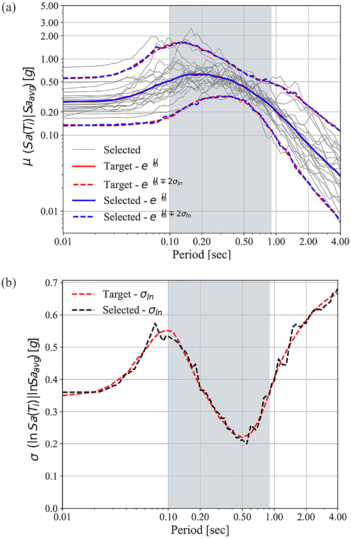
A discrete set of $n_{\mathrm{gm}}=\{5,10,20,30,40,60,80\}$ is used. Unlike the Caltrans design spectrum, CS contains two target spectra that are matched simultaneously. In this case, the strategy of ground motion selection used in the code-prescriptive assessment does not work, because a good match with the CMS does not guarantee a good match with the conditional standard deviation spectrum. Instead, we perform distinct ground motion selections at each $\mathrm{IM}$ level and each site. A total of $\mathrm{three}\mathrm{sites}\times \mathrm{six}\mathrm{IM}\mathrm{levels}\times n_{\mathrm{gm}}$ NRHAs are performed for each $n_{\mathrm{gm}}$ value. EzGM (Özsaraç, 2023) is used to automate the ground motion selection procedure. For illustration purposes, Figure 6 shows that the selected record-set matches the target CS for the 975-year return period at the Oakland site, with $n_{\mathrm{gm}}=20$ .

Figure 6.

Selection of 20 ground motions based on the CS for the Oakland site and 975-year return period. (a) Conditional mean matching and (b) conditional dispersion matching.

The mean annual frequency of exceeding a given limit state, ${\lambda }_{\mathrm{ls}}$ , is calculated by integrating the fragility function with the hazard curve:

$$\begin{array}{c}\multicolumn{1}{c}{{\lambda }_{\mathrm{ls}}={\int }_{\mathrm{im}}P(\mathrm{LS}>\mathrm{ls}|\mathrm{IM}=\mathrm{im})|d\lambda (\mathrm{im})|}\\ \multicolumn{1}{c}{\approx \sum _{i}P(\mathrm{LS}>\mathrm{ls}|\mathrm{IM}=\mathrm{im})|\lambda (i{m}_{i+1})-\lambda (i{m}_i)|.}\end{array}$$

(9)

The uncertainty in the hazard curve is not considered, that is, the mean hazard curve from PSHA is used. In this sense, the differences in the seismic hazard are constant, and the uncertainty only comes from the fragility term.

It is difficult to derive the moments of ${\lambda }_{\mathrm{ls}}$ analytically since the probability terms involve a function of random variables. Instead, Lallemant and Kiremidjian (2017) used the first-order second-moment approximation to estimate the mean and variance of the mean annual frequency:

$$\mathbb{E}({\lambda }_{\mathrm{ls}})\approx \sum _i\Phi (\mathbb{E}({\beta }_0+{\beta }_1\log i{m}_i))·|\lambda (i{m}_{i+1})-\lambda (i{m}_i)|,$$

(10a)

$$\mathbb{V}({\lambda }_{\mathrm{ls}})\approx \sum _{i,j}|\lambda (i{m}_{i+1})-\lambda (i{m}_i)||\lambda (i{m}_{j+1})-\lambda (i{m}_j)|{\rho }_{\mathrm{ij}}\sigma (p_i)\sigma (p_j),$$

(10b)

where $\sigma (p_i)$ is the standard deviation of $P(\mathrm{LS}>\mathrm{ls}|\mathrm{IM}=i{m}_i)$ , and ${\rho }_{\mathrm{ij}}$ is the correlation coefficient between $p_i$ and $p_j$ . Since $p_i$ and $p_j$ are expressed with the same GLM coefficients ${\beta }_0$ and ${\beta }_1$ , they are perfectly correlated and hence ${\rho }_{\mathrm{ij}}=1$ .

Figure 7 shows the $\mathrm{CV}$ estimates for the MAF of exceeding different limit states (expressed as $\frac{\sqrt{\hat{\mathbb{V}}({\lambda }_{\mathrm{ls}})}}{\hat{\mathbb{E}}({\lambda }_{\mathrm{ls}})}$ ) for ${\hat{\lambda }}_{\mathrm{ls}}$ for the slight, moderate, extensive, and collapse limit states, with $n_{\mathrm{gm}}=\{5,10,20,30,40,60,80\}$ used in each stripe, for the three design eras and three sites. Some of the $\mathrm{CV}$ estimates are not reported and are described as “uninformative” cases because almost all ground motions cause the bridge to exceed (or not) the associated limit state. The uninformative cases issue is further discussed later in this section.

Figure 7.

$\hat{\mathrm{C}}\mathrm{V}({\hat{\lambda }}_{\mathrm{ls}})$ for different limit states and $n_{\mathrm{gm}}$ values used at each $\mathrm{IM}$ level.

When model misspecification is ignored, $\hat{\mathrm{C}}{\mathrm{V}}^{\mathrm{IF}}({\hat{\lambda }}_{\mathrm{ls}})$ exhibits a decreasing trend as $n_{\mathrm{gm}}$ increases. Similar to the code-prescriptive assessment, this decreasing trend is not monotonic. When $n_{\mathrm{gm}}$ approaches 30, $\hat{\mathrm{C}}{\mathrm{V}}^{\mathrm{IF}}({\hat{\lambda }}_{\mathrm{ls}})$ tends to converge. However, it is obvious that model misspecification is prevalent. Figure 8 reports the $p$ -values from the information matrix test introduced before. Although in some cases the $p$ -values from the hypothesis testing are relatively high ( $p$ -value $>0.05$ ) and the $H_0$ is therefore not rejected, we still observe significant differences between the $\mathrm{CV}$ estimates from the two methods. For example, $\hat{\mathrm{C}}{\mathrm{V}}^{\mathrm{RB}}({\hat{\lambda }}_{\mathrm{ls}=\mathrm{Slight}})$ for the Era 1 bridge at the Malibu West site using 40 ground motions is nearly twice that of its IF counterpart. However, the evidence is not strong enough to reject $H_0$ (its $p$ -value = 0.27). This is because the selection of an appropriate significance level is subjective, and the choice of the $0.05$ significance level in this study may be unconservative.

Figure 8.

$p$ -Values from the information matrix test for different limit states versus $n_{\mathrm{gm}}$ used at each $\mathrm{IM}$ level.

The increase in the $\hat{\mathrm{C}}\mathrm{V}$ in the misspecification cases indicates a greater number of ground motions are required to achieve a target precision. For example, when ignoring the possibility of misspecification, using 5 ground motions at each $\mathrm{IM}$ level for the Era 1 bridge located at the Sacramento site is sufficient to lower the estimation uncertainty to the moderate variability level (with $\hat{\mathrm{C}}{\mathrm{V}}^{\mathrm{IF}}({\hat{\lambda }}_{\mathrm{ls}=\mathrm{Slight}})\le 0.3$ ). However, model misspecification increases this value to $0.4$ , which is 30% higher than the IF-based method. This indicates that at least 10 ground motions should be used to achieve the same precision. Similarly, $\hat{\mathrm{C}}{\mathrm{V}}^{\mathrm{RB}}({\hat{\lambda }}_{\mathrm{ls}=\mathrm{Slight}})$ for the Era 2 bridge located at the Malibu West site using 10 ground motions has two times the estimation uncertainty compared to its IF-based counterpart. In this situation, twice the number of ground motions is needed to limit $\hat{\mathrm{C}}\mathrm{V}$ to the moderate variability level.

The estimation uncertainty across different sites does not contain any clear trend. However, sites with low (Sacramento) and moderate (Malibu West) seismicity generally show higher estimation uncertainty than the site with the highest seismicity (Oakland) for the Era 1 and Era 2 bridges. In addition, in many cases, the $\hat{\mathrm{C}}\mathrm{V}({\hat{\lambda }}_{\mathrm{ls}})$ for slight and moderate limit states is higher than the more severe limit states (extensive and collapse). For the Era 1 and Era 2 bridges, 5 ground motions per stripe basically achieves a moderate variability level for the extensive and collapse limit states, and 30 ground motions are needed to reduce the estimation uncertainty to the low variability level. For slight and moderate damage, this number increases to 20 for moderate variability, and roughly 60 to achieve low variability. Also, there is no significant difference observed for $\hat{\mathrm{C}}\mathrm{V}({\hat{\lambda }}_{\mathrm{ls}})$ across different bridge design eras. This is particularly true for the IF-based method.

Discussion of the uninformative cases. $\hat{\mathrm{C}}\mathrm{V}({\hat{\lambda }}_{\mathrm{ls}})$ is not reported when uninformative observations are present. This happens when a bridge has very low capacity (e.g. slight limit state for the Era 1 design) and is subjected to high seismic demands (Oakland), or in bridges with very high capacity (e.g. collapse capacity of Era 3 bridges) located at a site with low seismic hazard (Sacramento). In these cases, the limit state exceedance counts are uninformative, meaning under all of the $\mathrm{IM}$ levels, nearly all ground motions cause the bridge to fail or survive. When this happens, the algorithm determines the probability of exceeding a limit state to be nearly deterministic with infinite estimation uncertainty. Thus, both the IF-based and the robust standard errors fail.

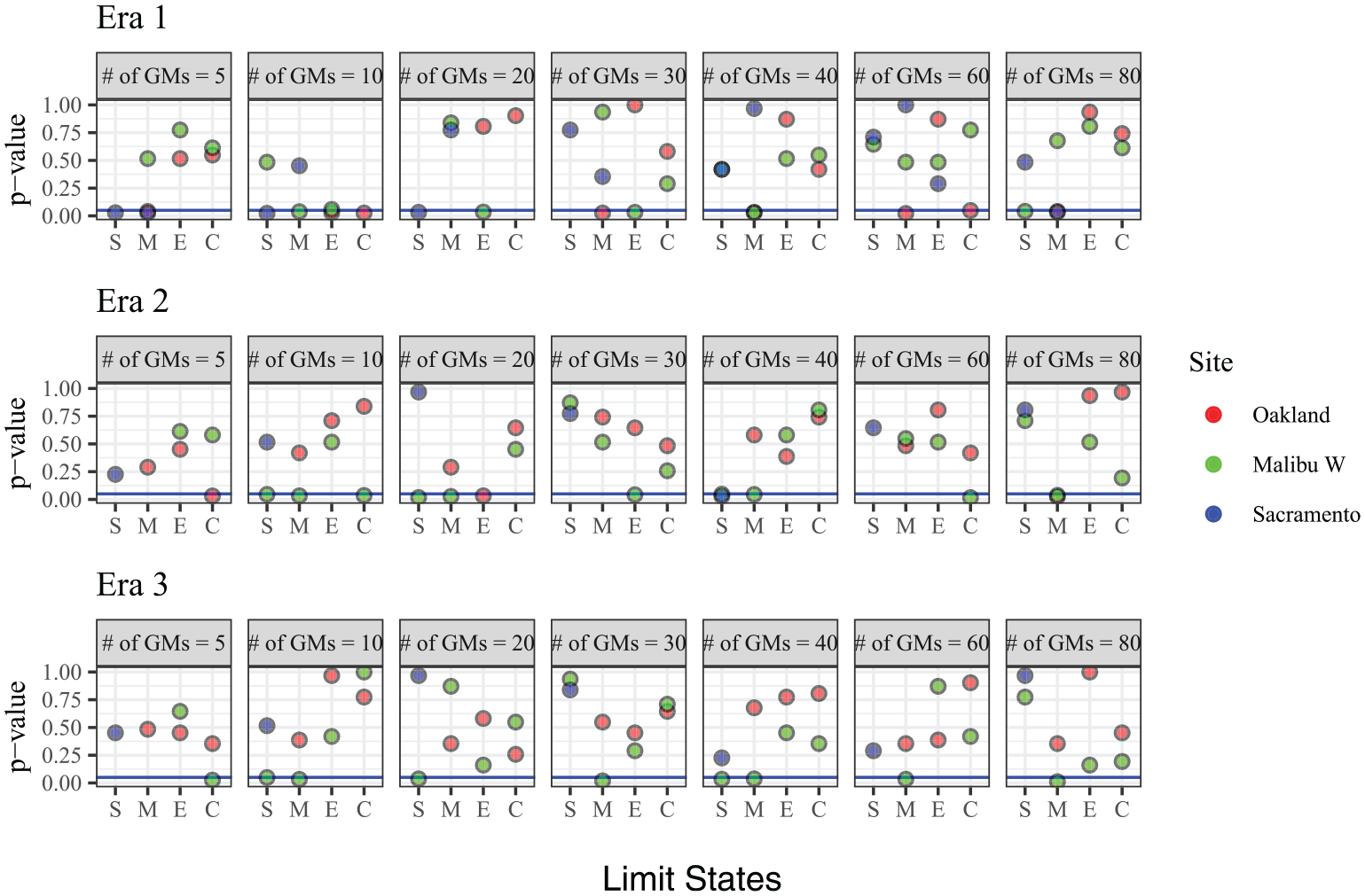
To better visualize the difference between the uninformative and informative cases, Figure 9 shows the log-likelihood surfaces as a function of the two GLM coefficients. The red points marked at the surface are the maximum likelihood estimates. Recall the observed information matrix or the bread matrix (shown in Equations A.14 and A.21 of the supplement, the negative second derivative of the log-likelihood function) essentially represents the curvature of the surface around the maximum likelihood estimator. A small curvature (the left panel) indicates low information carried by the data about the true parameters, and thereby high estimation uncertainty. Conversely, a high curvature (the right panel) implies low estimation uncertainty.

Figure 9.

Comparison of log-likelihood surfaces between (a) an uninformative case (Malibu West, Era 2, collapse) and (b) an informative case (Malibu West, Era1, extensive damage).

We propose several solutions to these uninformative observations:

• One can simply claim the structure is strong enough to resist any level of shaking up to the maximum considered $\mathrm{IM}$ level, or is incapable of resisting any shaking above the minimum considered $\mathrm{IM}$ level, according to the current structural design scheme and limit state. However, this claim is highly uncertain since there exists no more information above or below the $\mathrm{IM}$ levels under consideration.

• Incorporating even lower or higher $\mathrm{IM}$ levels into the MSA. This strategy may lead to effective exceedance counts (i.e. non-zero or non-one proportions) at extremely low or high $\mathrm{IM}$ levels. However, except for special structures (e.g. nuclear plants), in most cases, it is not necessary to consider extremely rare or common events. In this study, the selected $\mathrm{IM}$ levels with return periods ranging from 50 to 10,000 years are appropriate.

• Increasing the number of ground motions used in each stripe. The uninformative case may be due to the use of a very small sample size, which can easily lead to selection bias.

• Using an alternative structural analysis strategy. For example, cloud analysis (Jalayer et al., 2017), in which a greater number of unscaled ground motions are selected to match a single target spectrum at a fixed rate of exceedance. Since the ground motions are unscaled, the $\mathrm{IM}$ levels are continuous, and it is possible to obtain more effective counts than MSA. However, as suggested by Jalayer et al. (2017), a very careful ground motion selection should be performed to ensure a great portion of records leads to structural failures and the dispersion in the records’ intensity is considerable. We chose to use MSA coupled with CS because it is recognized to be a more efficient (Baker, 2015) and hazard-consistent (Chandramohan et al., 2016) strategy than the cloud analysis.

Conclusion

Estimation uncertainty is inevitable in seismic performance assessment procedures due to the use of a finite record-set size. The required number of ground motions for NRHAs is evaluated based on the precision of the statistical estimates of interest. To measure the precision of parameter estimates, inferential statistics that are based on standard errors of the parameter must be estimated from samples. This study introduces two types of standard errors which are derived based on the asymptotic normality of maximum likelihood estimators. One is based on the inverse of the Fisher information matrix, which does not consider misspecification potential. The other is the robust standard error that stems from QMLE theory which maintains asymptotic consistency even if the probability model is misspecified.

We develop a procedure that quantifies the estimation uncertainty in both code-prescriptive and risk-based performance assessments of California bridges. In the code-prescriptive assessment, we select varying numbers of ground motions $\left(n_{\mathrm{gm}}\right)$ that are consistent with the Caltrans SDC v2.0 design spectra. Choosing the CV of the median $(\mathrm{CV}(m_{\mathrm{EDP}|\mathrm{IM}}))$ and dispersion $(\mathrm{CV}({\sigma }_{\log (\mathrm{EDP})|\mathrm{IM}}))$ as target inferential statistics, we investigate the effects of $n_{\mathrm{gm}}$ on the estimation uncertainty in the column maximum curvature ductility $\left({\varphi }_m\right)$ . Specific observations are as follows:

• In general, misspecification is not detected in $m_{{\varphi }_m|\mathrm{IM}}$ . Using either the IF-based or robust standard errors yields the same $\hat{\mathrm{C}}\mathrm{V}({\hat{m}}_{{\varphi }_m|\mathrm{IM}})$ . However, misspecification is detected for dispersion estimates. The most severe case happens in a low seismic hazard zone, which increases the estimation uncertainty by a factor of 1.9 and leads to nearly twice the number of ground motions being needed to achieve a target precision.

• For $m_{{\varphi }_m|\mathrm{IM}}$ , a higher estimation uncertainty is observed in locations with high seismicity. For ${\sigma }_{\log ({\varphi }_m)|\mathrm{IM}}$ , we found that the $\mathrm{CV}$ estimates of any normally or lognormally distributed EDP are independent of specific sample values if misspecification potential is ignored. This means that analysts can immediately determine $n_{\mathrm{gm}}$ from the derived analytical formula in Supplement B without performing any upfront structural analyses. However, since misspecification is detected in dispersion estimates, we suggest using QMLE when the primary interest is in the precision of dispersion.

• The specification of a minimum of 7 ground motions in Caltrans SDC v2.0 for bridge design is evaluated. This minimum requirement is essentially sufficient to control the precision of the median EDP estimate at the low variability level and the estimation uncertainty for dispersion has moderate variability. If the goal is to have a more precise estimate of the dispersion, at least 20 ground motions should be selected.

In the risk-based assessment, we use MSA based on different sets of CS-consistent ground motions while varying the $n_{\mathrm{gm}}$ used in each stripe. Bridges with varying seismic capacities that were designed in different eras, and three sites in California with high, moderate, and low seismic hazard levels, are considered.

We choose the CV of the mean annual frequency of limit state exceedance $(\mathrm{CV}({\lambda }_{\mathrm{ls}}))$ as the target inferential statistic. Specific observations are as follows:

• Overlooking misspecification yields biased estimation uncertainty and hence an underestimated required number of ground motions. In contrast, using the robust standard error to amend estimation uncertainty when misspecification is present leads to a greater required record-set size. This is revealed by the fact that the cases detected as having misspecified probability models make the monotonic decreasing trend of estimation uncertainty as a function of sample size unstable.

• Generally, $\hat{\mathrm{C}}\mathrm{V}({\hat{\lambda }}_{\mathrm{ls}})$ for the slight and moderate limit states has higher uncertainty than for the more severe limit states. For the Era 1 and Era 2 bridges, roughly 5 and 30 ground motions are needed for the extensive damage and collapse limit states to attain the moderate and low variability levels, respectively. These numbers are increased to roughly 20 and 60 for the slight and moderate limit states, respectively. Also, sites with low and moderate seismicity generally show higher estimation uncertainty than the high seismicity site.

• The uninformative observations in the risk-based assessment are discussed, which occur when the limit state is exceeded (or not) for all or nearly all the ground motions and $\mathrm{IM}$ levels. When there are uninformative observations, the corresponding statistical inference is invalid. We propose several strategies to address this issue.

The procedure developed in this study can be used to detect model misspecification, quantify estimation uncertainty in seismic performance assessment procedures, and determine the number of ground motions that are required to yield a reliable estimate of the parameters of interest. We recommend analysts use QMLE to detect model misspecification and rectify the estimation uncertainty when misspecification is present. While the findings and conclusions from this study are specific to the considered bridges, the proposed framework can be implemented for other types of structures.

Supplemental Material

sj-pdf-1-eqs-10.1177_87552930241262044 – Supplemental material for Effects of probability model misspecification on the number of ground motions required for seismic performance assessment

Supplemental material, sj-pdf-1-eqs-10.1177_87552930241262044 for Effects of probability model misspecification on the number of ground motions required for seismic performance assessment by Chenhao Wu and Henry V Burton in Earthquake Spectra