A borehole array data–based approach for conducting 1D site response analyses I: Damping and V S randomization

Abstract

One-dimensional site response analysis (1D SRA) remains the state of practice to estimate site-specific seismic response, despite the ample evidence of discrepancies between observations and 1D SRA-based predictions. These discrepancies are due to errors in the input parameters, intrinsic limitations in the predicting capabilities of 1D SRAs even for sites relatively compliant with the 1D SRA assumptions, and the inability of 1D SRAs to model three-dimensional (3D) wave propagation phenomena. This article aims at reducing 1D SRA mispredictions using small-strain damping profiles factored by a damping multiplier (D_mul) and randomized shear-wave velocity (V_S) profiles. An approach for conducting 1D SRAs for site-specific site response assessment is developed to reduce the 1D SRA errors in magnitude and variability. First, sites from a database of 534 downhole sites are classified as 1D- or 3D-like, depending on the substructure conditions inferred from observed transfer functions. Second, data from the 1D-like sites are compared against predictions from 1D SRAs conducted using various trials of D_mul and V_S standard deviations $({\sigma }_{\ln V_S})$ for V_S randomization. Third, D_mul and ${\sigma }_{\ln V_S}$ are selected based on their combined ability to reduce the root mean square error (RMSE) in SRA predictions. Results indicate that 1D SRAs conducted with D_mul = 3 and ${\sigma }_{\ln V_S}=0.25$ lead to an overall minimum RMSE and thus provide more accurate site response estimates. The use of these parameters in forward SRA predictions is discussed in a companion paper.

Introduction

One-dimensional site response analysis (1D SRA) remains the state of practice to estimate site-specific seismic response, despite the ample evidence of discrepancies between observations from borehole array sites and 1D SRA predictions. These discrepancies are generally attributed to the lack of knowledge about the shear-wave velocity (V_S) profile, the breakdown of the 1D wave propagation assumptions, and three-dimensional (3D) effects (Hu et al., 2021; Kaklamanos et al., 2020; Stewart and Afshari, 2021). The parameterization of linear elastic 1D SRAs consists of damping and V_S profiles only. This simple parameterization and the broad implementation of 1D SRAs in practice prevent the addition of new parameters or adopting more advanced numerical approaches for estimating site response (e.g. Semblat, 2011). This situation leads to three alternatives for enhancing 1D SRA-based site response predictions: (1) altering the site response input parameters (V_S and damping); (2) post-processing 1D SRA estimates such that a more accurate site response is obtained, for example, using scaling factors; and (3) a combination of (1) and (2). In this work, an approach for conducting 1D SRAs for site-specific site response assessments for infrastructure is proposed. This approach uses damping profiles increased by a damping multiplier (D_mul), randomized V_S profiles, and a specific post-processing procedure to compute a site response that accounts for modeling limitations. This study focuses on linear elastic SRAs, henceforth referred to as “1D SRAs,” and thus only the small-strain damping is discussed and referred to as “damping” for brevity.

Current practices use geophysical testing and engineering correlations to define site response input parameters. In principle, both V_S and damping profiles could be measured using geophysical testing (e.g. Foti et al., 2014). However, damping is commonly estimated based on correlations with other geotechnical or seismological parameters (Boaga et al., 2015), while V_S profiles are often measured, although to an extent that is generally insufficient to understand and account for the V_S spatial variability and the potential presence of a complex geological structure underneath a site of interest. The approach for defining damping profiles in forward site response predictions remains a choice based on the analyst’s preference and available secondary data. These approaches include correlations with the site-specific attenuation parameter ${\kappa }_0$ (Xu et al., 2020); quality factors, Q (e.g. Cabas et al., 2017; Campbell, 2009; Olsen et al., 2003); and laboratory-based damping formulations (e.g. Darendeli, 2001; Menq, 2003). The latter are often scaled to better represent the extent of energy dissipation in field conditions (e.g. Rodriguez-Marek et al., 2017; Ruigrok et al., 2022; Tao and Rathje, 2019). The V_S spatial variability is the only site-specific feature intended to be addressed when conducting 1D SRAs in engineering practice. To this end, randomized V_S profiles generated using the Toro (1995) model are used (e.g. Griffiths et al., 2016a), and the mean response is considered as representative (e.g. Electric Power Research Institute (EPRI), 2013). However, studies show that this approach underpredicts the seismic response (Hallal et al., 2022; Kaklamanos et al., 2020; Pretell et al., 2022a; Tao and Rathje, 2019; Teague and Cox, 2016). To prevent these underpredictions, Pretell et al. (2022a) recommend using randomized V_S profiles generated using the model by Toro with V_S standard deviation $({\sigma }_{\ln V_S})=0.25$ and selecting the 84^th percentile seismic response as the representative at the site’s fundamental frequency.

The development of the approach herein proposed has two main parts. The first part consists of the selection of a D_mul to scale damping and a ${\sigma }_{\ln V_S}$ for V_S randomization, that together lead to the lowest minimum root mean square error (RMSE). The second part consists of the quantification of the 1D SRA remaining errors such that they can be considered in forward site response predictions. This article focuses on the first part, and the companion paper (Pretell et al., 2023) describes the second part.

Proposed approach for conducting 1D site response analyses

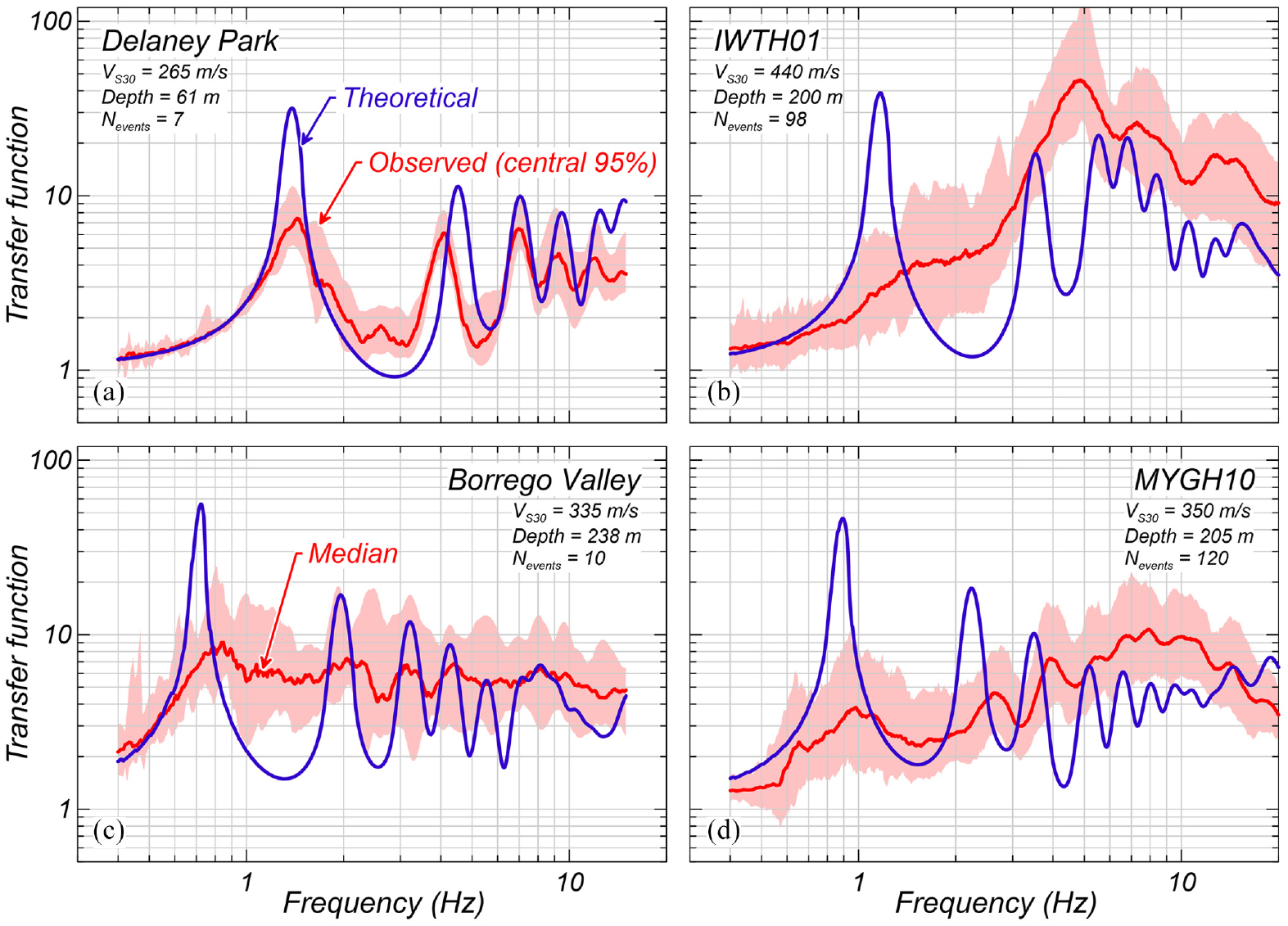
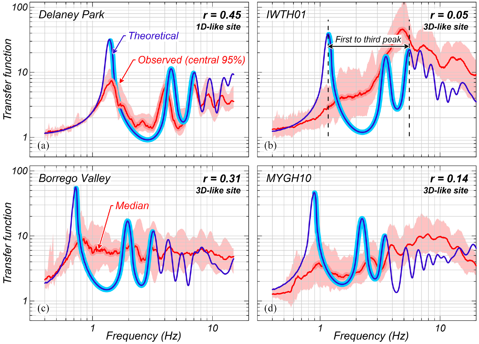
The state of practice for predicting site response uses 1D SRA as an approach that condenses the complexities of 3D wave propagation to an horizontally polarized vertically propagating shear (SH) wave traveling vertically through a soil column. Such simplification leads to modeling errors, evident when comparing 1D SRA predictions and observations (e.g. Bonilla et al., 2002; Kaklamanos and Bradley, 2018; Kaklamanos et al., 2013; Stewart and Afshari, 2021; Zhu et al., 2022). For example, Figure 1 shows the theoretical and observed transfer functions (TFs), defined as the ratio of the Fourier amplitude spectra at surface and depth, for four borehole array sites. Theoretical TFs are estimated considering a within boundary condition, to be consistent with observed TFs based on borehole array data (e.g. Kwok et al., 2007), and smoothed after Konno and Ohmachi (1998). Key observations in Figure 1 are (1) the overprediction of the theoretical fundamental mode (Figure 1a to d), (2) the underprediction of the high-frequency modes (Figure 1b to d), (3) the misalignment of the fundamental and higher frequency modes between the median observed and theoretical TFs (Figure 1b to d), and (4) the overall smoother observed TFs compared to the more sharply peaked theoretical TFs (Figure 1b to d). The commonly observed overprediction of the fundamental mode suggests that 1D SRAs have a consistent bias at the fundamental frequency, and less clearly so at higher frequencies (e.g. Kaklamanos et al., 2013). These trends are also observed for amplification factors (AFs), herein defined as the ratio of the pseudo-spectral acceleration (PSA) response spectra at surface and depth (within), although with milder under- and overpredictions given that the PSA at a single oscillator frequency has contributions from waves of multiple frequencies (Bora et al., 2016). In this section, an approach for conducting 1D SRAs with D_mul and V_S randomization is described.

Figure 1.

Comparison of observed and theoretical transfer functions (TFs). TFs computed using the measured V_S profiles and small-strain damping after Darendeli (2001). TFs plotted within the range of usable frequencies based on the signal-to-noise ratio.

Damping multipliers and V_S randomization in 1D SRAs

Various mechanisms lead to dissipation of energy during wave propagation, such as friction between particles and wave scattering, which are not modeled but can be captured by damping in 1D SRAs. Laboratory-based damping models (e.g. Darendeli, 2001; Menq, 2003) provide estimates of the intrinsic material damping and do not account for energy dissipation mechanisms existing in the field. As such, damping is underestimated, and the site response amplitudes are overestimated. Various authors propose that laboratory-based damping could be factored to improve site response predictions (Elgamal et al., 2001; Kokusho, 2017; Stewart et al., 2014; Tao and Rathje, 2019; Tsai and Hashash, 2009; Zalachoris and Rathje, 2015). For instance, Tao and Rathje (2019) find that D_mul = 3–5 applied to damping profiles after Darendeli (2001) reduces the discrepancies between observations and 1D SRA predictions at four borehole array sites, and Ruigrok et al. (2022) suggest that a D_mul = 0.65–1.6 can be used to scale laboratory damping-based ${\kappa }_0$ to match Q estimates at the Groningen gas field in the Netherlands.

Randomized V_S profiles generated using the Toro (1995) model for 1D SRA applications are commonly used in the nuclear industry (e.g. Abrahamson et al., 2002, 2004; Bommer et al., 2015; EPRI, 2013; Rodriguez-Marek et al., 2021). Toro recommends different ${\sigma }_{\ln V_S}$ values for V_S randomization ranging from 0.27 to 0.37, depending on site classes determined based on V_S30, estimated as the inverse of the average slowness in a site’s top 30 m. Generally, V_S profiles are randomized with the goals (1) to reduce the overpredictions at the site’s fundamental mode (e.g. Figure 2c) and (2) to capture the V_S spatial variability across the footprint of a project site. However, it is unclear how the amount of randomization mapped through ${\sigma }_{\ln V_S}$ should vary for sites with different site-specific conditions regardless of V_S30 (e.g. V_S variability, subsurface structure). Overall, various studies indicate that the ${\sigma }_{\ln V_S}$ values recommended by Toro are excessively high and thus V_S randomization leads to unrealistically low site response estimates (e.g. Griffiths et al., 2016b; Passeri et al., 2020; Stewart et al., 2014; Tao and Rathje, 2019; Teague et al., 2018). Pretell et al. (2022a) show that not only ${\sigma }_{\ln V_S}$ is generally too high, but site response underpredictions also originate from considering the median site response as representative. Based on a numerical investigation, Pretell et al. (2022a) suggest that the 84^th percentile site response from 1D SRAs conducted with randomized V_S profiles $({\sigma }_{\ln V_S}=0.25)$ is an appropriate response that accounts for V_S spatial variability at the site’s fundamental frequency.

Figure 2.

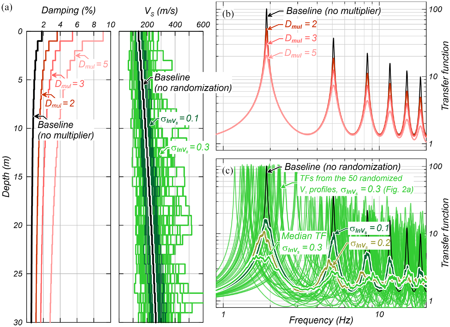
Effects of increased damping and randomized V_S profiles on transfer functions (TFs) in 1D site response analyses: (a) Damping and randomized V_S profiles. (b) Effect of damping on TFs for various damping multipliers (D_mul). (c) Effect of V_S randomization on TFs for various V_S standard deviations ( ${\sigma }_{\ln {\mathrm{V}}_{\mathrm{S}}}$ ). Baseline TFs computed using the small-strain damping after Darendeli (2001). Baselined V_S profile randomized using the Toro (1995)V_S model.

Increasing damping and randomizing V_S profiles are both tools that affect the estimated responses differently but can be used to improve 1D SRA predictions. For instance, Figure 2 shows TFs calculated for various D_mul and ${\sigma }_{\ln V_S}$ values applied to a baseline V_S profile generated after Kamai et al. (2016) for site conditions consistent with California. As observed, both D_mul and ${\sigma }_{\ln V_S}$ reduce the site response amplitudes at the fundamental mode, but the D_mul causes a stronger reduction in the high-frequency range (Figure 2b), whereas ${\sigma }_{\ln V_S}$ leads to relatively stable minimum amplitudes (Figure 2c).

Approach for improving site response predictions

In theory, 1D SRAs should provide the best possible site response predictions for sites that are more compatible with 1D SRA assumptions (1D-like sites), while larger errors are expected for sites that are more strongly affected by non-1D effects (3D-like sites). However, the assumptions of the 1D SRA approach are unrealistic and thus 1D SRAs cannot predict site response accurately even for 1D-like sites, or cases with V_S profiles exempt from measurement errors, as demonstrated in numerical investigations (e.g. de la Torre et al., 2021; Pretell et al., 2022b). Such errors are herein referred to as “intrinsic errors.” Two major sources of such errors are (1) the unrealistic wave reverberations and spurious resonances that lead to overpredictions of the amplitudes at the sites’ fundamental frequency (Boore, 2013) and (2) the inability to simulate energy dissipation mechanisms, thus leading to an overall overprediction of site response amplitudes. It is hypothesized that the portion of 1D SRA mispredictions due to intrinsic 1D-SRA errors can be removed using randomized V_S profiles and an increased amount of damping. The remaining residuals can then be attributed to 3D effects affecting the seismic response, the intrinsic complexity of the wave propagation phenomena, and randomness of ground motion waveforms.

An approach for conducting 1D SRAs using increased damping and randomized V_S profiles is proposed with two objectives: (1) to remove the bias intrinsically carried by 1D SRAs following the previously described hypothesis and (2) to obtain the minimum variance in site response residuals and improve site response predictions across frequencies overall. To achieve these goals, this study builds off the work by Tao and Rathje (2019) and Pretell et al. (2022a) to find the most appropriate D_mul and ${\sigma }_{\ln V_S}$ by comparing 1D SRA predictions to ground motion data from 1D-like borehole array sites, whose intrinsic errors in 1D SRAs are more clearly identified. Pretell et al. (2022a) hypothesized that V_S randomization can be treated as a multi-purpose tool used to capture site-specific features affecting the seismic response such as (1) V_S spatial variability (e.g. Assimaki et al., 2003; de la Torre et al., 2021; El Haber et al., 2019; Nour et al., 2003; Pretell et al., 2022a); (2) a dipping bedrock and topography (e.g. Katebi et al., 2018), wave inclination (e.g. Semblat et al., 2000; Zhu et al., 2016); and (3) other features that cannot be explicitly modeled in 1D SRAs (e.g. edge effects). This approach is extended to find the right amount of ${\sigma }_{\ln V_S}$ for V_S randomization that along with D_mul (1) removes the intrinsic errors associated to 1D SRAs, and (2) reduces the amount of mispredictions caused by the effects of site-specific features uncaptured by 1D SRAs. This does not prevent the potential for including a higher or lower amount of V_S randomization to capture specific features (e.g. V_S variability, topographic effects), but further work is needed in this direction. The use of D_mul in 1D SRAs follows a similar reasoning, motivated by the inability to explicitly model energy dissipation mechanisms in 1D SRAs.

Framework of aleatory variability and epistemic uncertainty

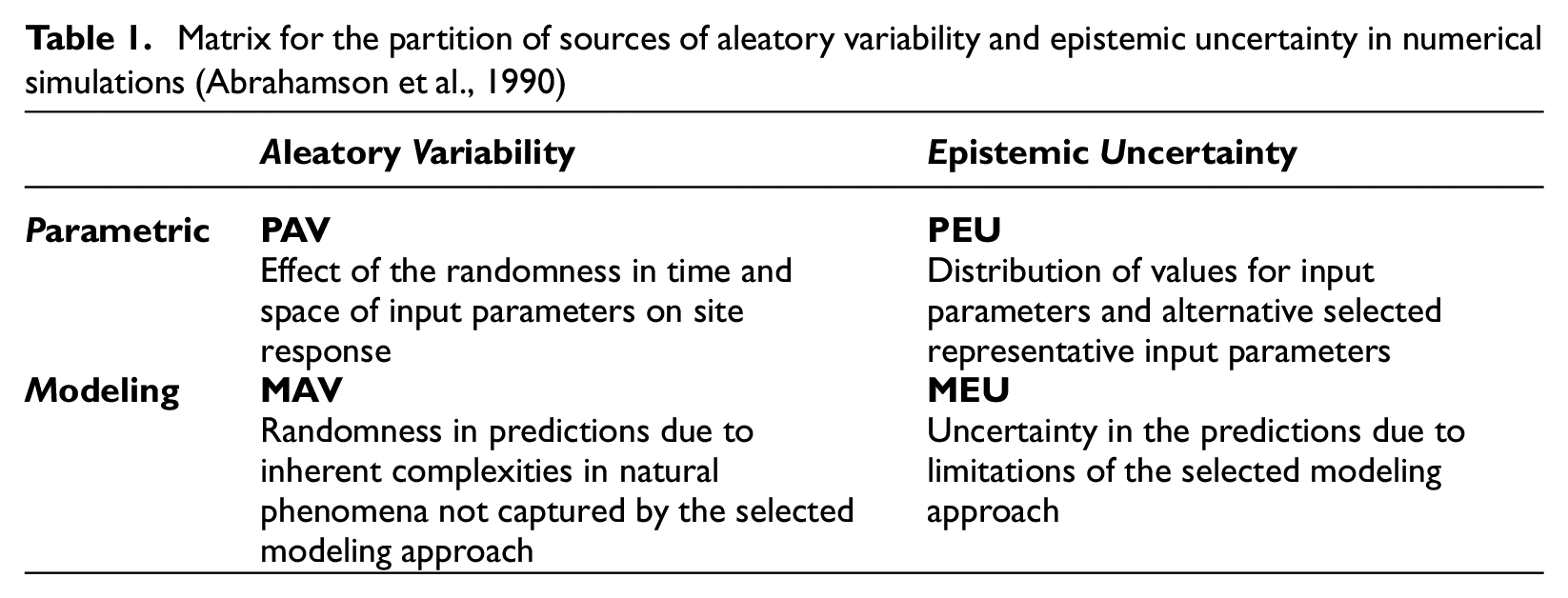
One-dimensional SRAs, or more generally numerical simulations and analysis tools, inevitably deal with sources of aleatory variability (AV) and epistemic uncertainty (EU) as described by Abrahamson et al. (1990) and Roblee et al. (1996). AV and EU refer to variability due to apparent randomness of the natural phenomena caused by the features uncaptured in a selected modeling approach, and the lack of knowledge about the optimal input parameters, respectively (Abrahamson et al., 2004; Baecher and Christian, 2003). Abrahamson et al. (1990) further partitioned the AV and EU into parametric and modeling components (Table 1). The parametric aleatory variability (PAV) results from the spatial and temporal randomness of the input parameters, whereas the parametric epistemic uncertainty (PEU) results from the lack of knowledge about the ranges of input parameters and the values sampled for analyses. The modeling aleatory variability (MAV) is due to the site-specific features whose effects are not captured by the analysis tool, and the modeling epistemic uncertainty (MEU) is due to the limited predictive capabilities of the analysis tool.

Table 1.

Matrix for the partition of sources of aleatory variability and epistemic uncertainty in numerical simulations (Abrahamson et al., 1990)

	Aleatory Variability	Epistemic Uncertainty
Parametric	PAV Effect of the randomness in time and space of input parameters on site response	PEU Distribution of values for input parameters and alternative selected representative input parameters
Modeling	MAV Randomness in predictions due to inherent complexities in natural phenomena not captured by the selected modeling approach	MEU Uncertainty in the predictions due to limitations of the selected modeling approach

Generally, there is a trade-off between the complexity of the analysis tool and the MAV. For instance, within the context of ground motion modeling, it is expected that ground motion models (GMMs) that only account for magnitude and distance (i.e. a simple parameterization) have a larger MAV than GMMs that also account for site conditions mapped through V_S30 and the depth to V_S = 1 km/s, Z₁ (i.e. a more complex parameterization). The reduction in MAV for the second GMM comes with an additional PEU associated with the V_S30 and Z₁ scaling in the model that can be reduced as larger data sets are collected, or if additional investigations are conducted to better estimate such parameters. Overall, there is a benefit in trading MAV for PEU as the latter can be reduced, whereas the former can only be accounted for.

The framework proposed by Abrahamson et al. (1990) can be adapted to 1D SRA applications. The PAV consists of random factors affecting site response that can be explicitly modeled. The PAV includes the ground motion waveforms, an example of randomness in time, and V_S spatial variability, an example of randomness in space. The PEU consists of the plausible alternative input parameters, selected based on some criteria, such as a given mean and standard deviation of ground motion spectral accelerations, and best-estimate, lower, and upper bound V_S profiles. A part of MAV can be reduced as site-specific terms are quantified (more complex model). Finally, the remaining part of MAV consists in the variability of site response given its natural randomness that is not captured by the selected modeling approach, for example, ground motion inclination within the context of 1D SRAs.

Site response residual components

The errors carried by 1D SRA predictions can be quantified using borehole array data, which consist of ground motion recordings at depth and ground surface. In 1D SRAs, the ground motions recorded at depth are expected to explain the ground motions at surface assuming that the site’s 1D V_S profile is accurate. Thus, the recordings at depth can be used as input motions and the resulting responses at surface be compared against the ground surface recordings to evaluate the accuracy of 1D SRAs. For an intensity measure “ $\mathrm{IM}$ ” estimated using 1D SRAs, and the corresponding observed earthquake component “e” at a site “s,” the following relation can be established:

$${\mathrm{IM}}_{\mathrm{es}}^{\mathrm{obs}}={\mathrm{IM}}_{\mathrm{es}}^{\mathrm{SRA}}+{\delta }_{\mathrm{es}}^{\mathrm{SRA}}$$

(1)

where ${\mathrm{IM}}_{\mathrm{es}}^{\mathrm{obs}}$ and ${\mathrm{IM}}_{\mathrm{es}}^{\mathrm{SRA}}$ are, respectively, the observed and 1D SRA-predicted $\mathrm{IM}$ in natural logarithm units, and ${\delta }_{\mathrm{es}}^{\mathrm{SRA}}$ is the 1D site response residual. $\mathrm{IM}$ can represent TFs, AFs, or any other metric of interest. Following the separation of residuals proposed by Al Atik et al. (2010), adapted to the approach for conducting 1D SRAs herein proposed, the residual in Equation 1 can be expressed as follows:

$${\delta }_{\mathrm{es}}^{\mathrm{SRA}}=c^{\mathrm{SRA}}+\delta 1{\mathrm{D}}_s^{\mathrm{SRA}}+\delta 3{\mathrm{D}}_{\mathrm{es}}^{\mathrm{SRA}}$$

(2)

where $c^{\mathrm{SRA}}$ is the global 1D SRA bias, $\delta 1{\mathrm{D}}_s^{\mathrm{SRA}}$ is the site-specific residual due to intrinsic 1D-SRA errors (e.g. the 1D SRA overprediction at the site’s fundamental mode), and $\delta 3{\mathrm{D}}_{\mathrm{es}}^{\mathrm{SRA}}$ is the residual due to non-1D features affecting the site response and the effect of different ground motion waveforms that are not accounted for by $c^{\mathrm{SRA}}$ . The residual $\delta 3{\mathrm{D}}_{\mathrm{es}}^{\mathrm{SRA}}$ can be further partitioned as follows:

$$\delta 3{\mathrm{D}}_{\mathrm{es}}^{\mathrm{SRA}}=\delta \mathrm{S}2{\mathrm{S}}_{\mathrm{s}}^{\mathrm{SRA}}+\delta {\mathrm{AMP}}_{\mathrm{es}}^{\mathrm{SRA}}$$

(3)

where $\delta \mathrm{S}2{\mathrm{S}}_s^{\mathrm{SRA}}$ is the site-specific error in the analytical modeling, estimated as the mean bias-corrected residual at a site “s,” and $\delta {\mathrm{AMP}}_{\mathrm{es}}^{\mathrm{SRA}}$ is the unexplained remaining bias- and site-corrected residual. The components $\delta \mathrm{S}2{\mathrm{S}}_{\mathrm{s}}^{\mathrm{SRA}}$ and $\delta {\mathrm{AMP}}_{\mathrm{es}}^{\mathrm{SRA}}$ are considered random variables with zero mean and standard deviations ${\varphi }_{\mathrm{S}2\mathrm{S}}^{\mathrm{SRA}}$ and ${\varphi }_{\mathrm{AMP}}^{\mathrm{SRA}}$ , respectively. Replacing Equation 3 into Equation 2,

$${\delta }_{\mathrm{es}}^{\mathrm{SRA}}=c^{\mathrm{SRA}}+\delta 1{\mathrm{D}}_s^{\mathrm{SRA}}+\delta \mathrm{S}2{\mathrm{S}}_s^{\mathrm{SRA}}+\delta {\mathrm{AMP}}_{\mathrm{es}}^{\mathrm{SRA}}$$

(4)

Equations 1, 2, and 4 correspond to 1D SRAs conducted with a single best-estimate V_S profile and an uncalibrated amount of damping (e.g. based on laboratory measurements or correlations with Q). Following the hypothesis herein proposed, $\delta 1{\mathrm{D}}_s^{\mathrm{SRA}}$ can be removed using the right amount of (i.e. calibrated) damping and V_S randomization through D_mul and ${\sigma }_{\ln V_S}$ , respectively. Therefore, using calibrated D_mul and ${\sigma }_{\ln V_S}$ , Equation 4 reduces to the following:

$${\delta }_{\mathrm{es}}^{\mathrm{SRA}}=c^{\mathrm{SRA}}+\delta \mathrm{S}2{\mathrm{S}}_s^{\mathrm{SRA}}+\delta {\mathrm{AMP}}_{\mathrm{es}}^{\mathrm{SRA}}$$

(5)

Note that ${\delta }_{\mathrm{es}}^{\mathrm{SRA}}$ in Equations 2 to 4 is calculated from Equation 1 with ${\mathrm{IM}}_{\mathrm{es}}^{\mathrm{SRA}}$ resulting from a V_S profile and an input ground motion. Differently, ${\delta }_{\mathrm{es}}^{\mathrm{SRA}}$ in Equation 5 is calculated from Equation 1 with ${\mathrm{IM}}_{\mathrm{es}}^{\mathrm{SRA}}$ representing the median $\mathrm{IM}$ resulting from a suite of randomized V_S profiles and an input ground motion. Thus, $c^{\mathrm{SRA}}$ in Equations 4 and 5 are conceptually different. This article aims at finding the D_mul and ${\sigma }_{\ln V_S}$ based on comparisons with borehole array data. Borehole array sites considered in the evaluation are those identified as 1D-like, thus $c^{\mathrm{SRA}}$ is expressed as $c_{1\mathrm{D}}^{\mathrm{SRA}}$ . The more common $c_{3\mathrm{D}}^{\mathrm{SRA}}$ , that is, the bias associated with 3D-like sites, the residual components $\delta \mathrm{S}2{\mathrm{S}}_s^{\mathrm{SRA}}$ and $\delta {\mathrm{AMP}}_{\mathrm{es}}^{\mathrm{SRA}}$ are discussed in the companion paper. All the terms in Equations 1 to 5 are frequency-dependent.

Various sets of SRAs are conducted for D_mul from 1 to 10 in increments of 1, and ${\sigma }_{\ln V_S}$ from 0.05 to 0.40 in increments of 0.05, leading to a total of 80 D_mul- ${\sigma }_{\ln V_S}$ trials. Ten additional sets of SRAs with D_mul from 1 to 10 and no V_S randomization are conducted. When randomization is used, a suite of 50 randomized V_S profiles is generated per site, and the median of the corresponding 50 theoretical TFs is compared against each of the observed TFs. In the case of AFs, each ground motion recording is propagated through the 50 V_S profiles resulting in 50 AFs per recording available. The median of these 50 theoretical AFs is compared against each of the observed AFs. In all cases, the randomized V_S profiles are generated using the model by Toro (1995) with the trial ${\sigma }_{\ln V_S}$ and all the other parameters originally recommended by Toro for sites with V_S30 from 180 to 360 m/s.

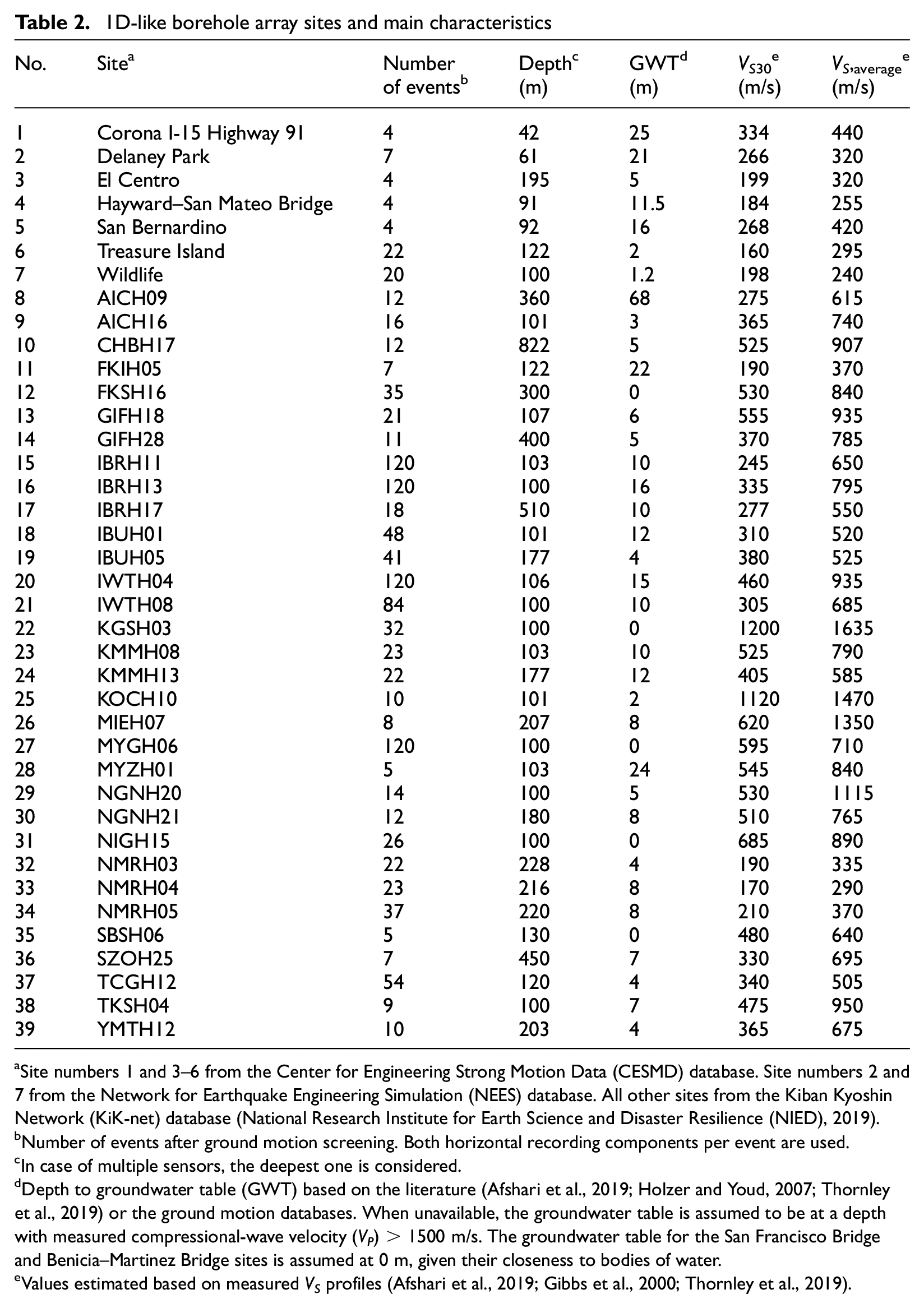
Several modeling decisions are considered for the damping and the V_S profiles. Damping profiles are calculated as a function of vertical effective stress following the formulation by Darendeli (2001) considering the same layering as in the V_S profiles. The Darendeli model is used assuming a plasticity index (PI) = 0, a load frequency (f_load) = 1 Hz, and a coefficient of lateral pressure at rest (K₀) = 0.5. The vertical effective stress is estimated considering the measured groundwater table level, when available, or water table depths inferred based on the deepest location with a compressional-wave velocity (V_P) higher than 1500 m/s (Table 2) or site conditions (e.g. closeness to a body of water). The sites’ mean effective stresses at the borehole sensor locations range approximately from 4.5 to 53 atm (assuming a K₀ = 0.5), with a 90^th percentile of 27.6 atm, which approximately falls within the range of isotropic confining pressures considered by Darendeli in the development of the model, from 0.3 to 27 atm. Sites with higher mean effective stresses are AICH09, CHBH17, IBRH17, and SZOH25. Randomized V_S profiles are generated based on measured V_S profiles using the V_S model by Toro (1995) with a with a constant σ_lnVS with depth, and the coefficients recommended for sites with V_S30 = 180–360 m/s, which are approximately the same as the coefficients for sites with V_S30 = 360–760 m/s, thus covering a wide range of shallow conditions. The correlation between damping and V_S is not considered in the estimation of damping or randomized V_S profiles. Instead, the same damping profile is used for all the randomized V_S profiles, given that V_S is randomized to reduce the 1D-SRA intrinsic errors (e.g. spurious resonances) rather than capturing the spatial variability of soil properties within a project footprint or an area of interest.

Table 2.

1D-like borehole array sites and main characteristics

No.	Site a	Number of events b	Depth c (m)	GWT d (m)	VS30 e (m/s)	VS,average e (m/s)
1	Corona I-15 Highway 91	4	42	25	334	440
2	Delaney Park	7	61	21	266	320
3	El Centro	4	195	5	199	320
4	Hayward–San Mateo Bridge	4	91	11.5	184	255
5	San Bernardino	4	92	16	268	420
6	Treasure Island	22	122	2	160	295
7	Wildlife	20	100	1.2	198	240
8	AICH09	12	360	68	275	615
9	AICH16	16	101	3	365	740
10	CHBH17	12	822	5	525	907
11	FKIH05	7	122	22	190	370
12	FKSH16	35	300	0	530	840
13	GIFH18	21	107	6	555	935
14	GIFH28	11	400	5	370	785
15	IBRH11	120	103	10	245	650
16	IBRH13	120	100	16	335	795
17	IBRH17	18	510	10	277	550
18	IBUH01	48	101	12	310	520
19	IBUH05	41	177	4	380	525
20	IWTH04	120	106	15	460	935
21	IWTH08	84	100	10	305	685
22	KGSH03	32	100	0	1200	1635
23	KMMH08	23	103	10	525	790
24	KMMH13	22	177	12	405	585
25	KOCH10	10	101	2	1120	1470
26	MIEH07	8	207	8	620	1350
27	MYGH06	120	100	0	595	710
28	MYZH01	5	103	24	545	840
29	NGNH20	14	100	5	530	1115
30	NGNH21	12	180	8	510	765
31	NIGH15	26	100	0	685	890
32	NMRH03	22	228	4	190	335
33	NMRH04	23	216	8	170	290
34	NMRH05	37	220	8	210	370
35	SBSH06	5	130	0	480	640
36	SZOH25	7	450	7	330	695
37	TCGH12	54	120	4	340	505
38	TKSH04	9	100	7	475	950
39	YMTH12	10	203	4	365	675

a

Site numbers 1 and 3–6 from the Center for Engineering Strong Motion Data (CESMD) database. Site numbers 2 and 7 from the Network for Earthquake Engineering Simulation (NEES) database. All other sites from the Kiban Kyoshin Network (KiK-net) database (National Research Institute for Earth Science and Disaster Resilience (NIED), 2019).

b

Number of events after ground motion screening. Both horizontal recording components per event are used.

c

In case of multiple sensors, the deepest one is considered.

d

Depth to groundwater table (GWT) based on the literature (Afshari et al., 2019; Holzer and Youd, 2007; Thornley et al., 2019) or the ground motion databases. When unavailable, the groundwater table is assumed to be at a depth with measured compressional-wave velocity (V_P) > 1500 m/s. The groundwater table for the San Francisco Bridge and Benicia–Martinez Bridge sites is assumed at 0 m, given their closeness to bodies of water.

e

Values estimated based on measured V_S profiles (Afshari et al., 2019; Gibbs et al., 2000; Thornley et al., 2019).

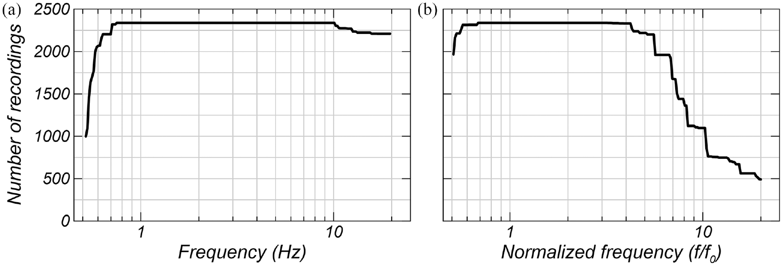
The theoretical TFs are computed using the computer code NRATTLE, while observed TFs are based on borehole array data. NRATTLE is included in the SMSIM program package (Boore, 2005). NRATTLE uses the Thomson–Haskell solution to compute the 1D SH-wave TF (Haskell, 1953; Thomson, 1950) based on profiles of V_S, density, and the inverse of the Q, estimated as half the inverse of damping (Joyner and Boore, 1988). PSAs (5% damping) are computed using pyRotD (Kottke, 2018). Only data from borehole array sites with measured V_S profiles are used, and it is assumed that such profiles are accurate. Ground motion recordings are screened and those with a shear strain index, $I_{\gamma }$ (Idriss, 2011) lower than 0.005%, expected to yield shear strains lower than 0.01% on average (Kim et al., 2016), are considered appropriate for linear elastic SRAs (Kaklamanos et al., 2013) and selected for this investigation. The ground motions are also screened to meet an acceptable signal-to-noise ratio (SNR) within frequencies higher than half the site’s fundamental frequency $(f_0)$ to a maximum frequency of 20 Hz. The maximum $I_{\gamma }$ and the minimum frequency bandwidth criteria are relaxed for sites in the United States given the limited amount of data available. For such sites, a maximum $I_{\gamma }$ of 0.01% and a maximum frequency up to 10–12 Hz are considered acceptable for SNR screening. This $I_{\gamma }$ is not uncommon in similar studies using ground motion data from the United States (e.g. Stewart and Afshari, 2021; Tao and Rathje, 2020), whereas a maximum frequency of 10 Hz for SNR screening does not impact on the amount of data at the high-frequency range (Figure 3a). The number of ground motions per usable (i.e. appropriate) SNR is presented as a function of frequencies and normalized frequencies $(f/f_0)$ in Figure 3 and summarized in Table 2. Note that the $f_0$ corresponds to the first mode of the theoretical TFs computed considering a within-motion boundary condition.

Figure 3.

Number of usable ground motion recordings per frequency (a) and per frequency normalized by the site’s fundamental frequency (b).

Identification of 1D-like sites

Several approaches for identifying sites compatible with the 1D SRA assumptions are available in the literature (Afshari and Stewart, 2019; Laurendeau et al., 2018; Pilz and Cotton, 2019; Pilz et al., 2022; Tao and Rathje, 2020; Thompson et al., 2012) as summarized by Hallal et al. (2022). For instance, Thompson et al. (2012) assessed a site’s compliance with the 1D SRA assumptions through the inter-event variability $(\mathrm{\sigma })$ and Pearson’s correlation coefficient $(r)$ between observed and theoretical TFs. The authors suggested that sites with $\sigma <0.35$ and $r>0.6$ are less exposed to 3D effects, and thus appropriately modeled using 1D SRAs.

In this work, sites with theoretical TFs estimated using D_mul = 1 and no randomization whose peaks align well with those in observed TFs are considered 1D-like. To evaluate this, an approach similar to the one proposed by Thompson et al. (2012) is followed, with the difference that only Pearson’s correlation coefficient is used. The goal of the evaluation is to find 1D-like sites that can be used for the calibration of D_mul and ${\sigma }_{\ln V_S}$ and thus remove the $\delta 1{\mathrm{D}}_s^{\mathrm{SRA}}$ component in Equation 4. Therefore, the inter-event variability, indicative of the azimuthal variations in the velocity structure (Pilz et al., 2022; Ramos-Sepúlveda and Cabas, 2021), is not used in the evaluation. The correlation coefficient is computed at five frequency ranges: (1) from the first to the second TF peak, (2) from the first to the third TF peak (e.g. Figure 4b), (3) from the first to the fourth TF peak, (4) from the second to the third TF peak, and (5) from the third to the fourth TF peak. In all cases, the maximum frequency was limited to the maximum usable frequency, based on the SNR. Multiple frequency intervals are used as opposed to a single broad range to prevent a single highly or negligibly correlated first mode from dominating the site selection, and thus identify 1D-like sites with a proper alignment of TF peaks across frequencies. A hundred sites with the highest Pearson’s correlation coefficients in at least three frequency intervals are initially selected as 1D-like candidates from a database of 534 borehole array sites from Japan and the United States. After a visual inspection, 39 sites are identified as 1D-like, which represents about 7% of the database. Examples of 1D- and 3D-like sites’ TFs are presented in Figure 4. A summary of the main characteristics of the 1D-like sites is presented in Table 2, the correlation coefficients in Supplemental Appendix A, and TFs and AFs estimated using D_mul = 1 and no randomization in Supplemental Appendices B and C.

Figure 4.

Example of 1D- and 3D-like sites. Pearson’s correlation coefficient $(r)$ between the observed and theoretical transfer functions from the first to the third peak of the theoretical transfer functions. No specific correlation coefficient threshold is used to distinguish 1D- from 3D-like sites.

Selection of D_mul and σ_lnVS

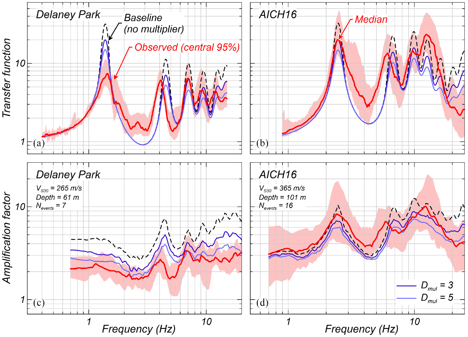
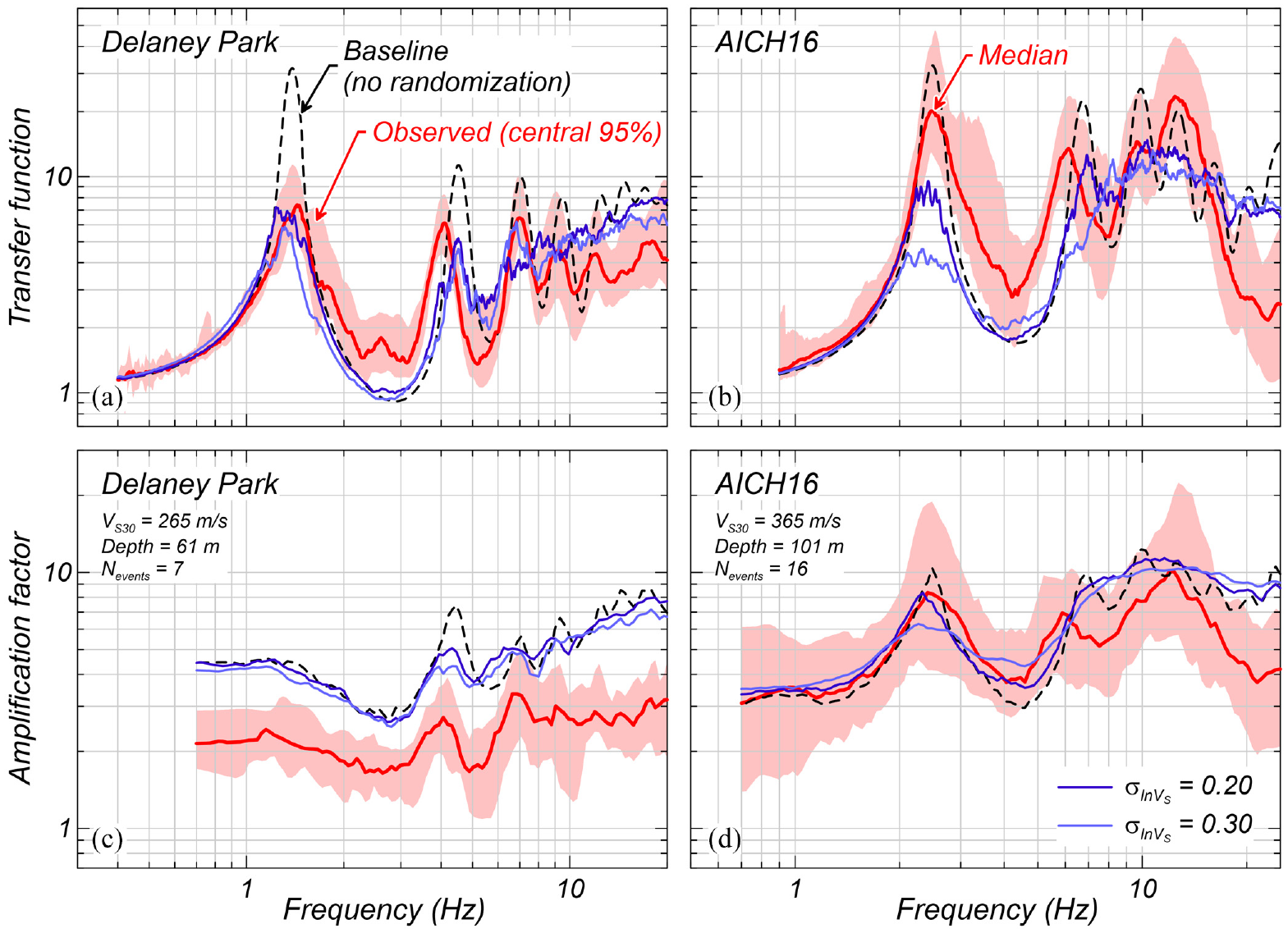
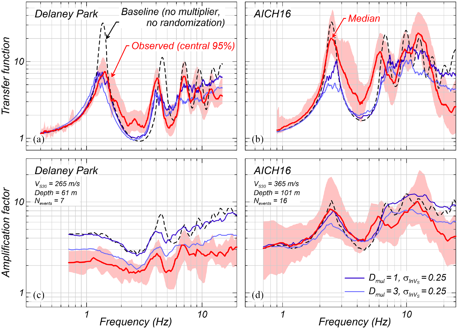
Both D_mul and ${\sigma }_{\ln V_S}$ can be used to improve 1D-SRA predictions in terms of TFs and AFs. The effect of increasing the small-strain damping by two D_mul, the effect of using V_S randomization with two ${\sigma }_{\ln V_S}$ , and the combined effect of D_mul and ${\sigma }_{\ln V_S}$ on TFs and AFs are presented in Figures 5 to 7 for the Delaney Park and the AICH16 sites. Several global trends are observed in these examples. For instance, increasing the small-strain damping by D_mul reduces the overprediction of TFs and AFs at the fundamental mode (e.g. Figure 5a and b), but it might also lead to underpredictions (e.g. Figure 5a for D_mul = 5). This is often the case for the high-frequency range, which is commonly underpredicted even for a non-scaled small-strain damping (or D_mul = 1) and no V_S randomization (e.g. Figure 5b around 13 Hz). Meanwhile, V_S randomization reduces the fundamental mode without significantly reducing the high-frequency range (e.g. Figure 6a to d), but it might not reduce enough the amount of overprediction observed at some sites (e.g. Figure 6c). The effectiveness of V_S randomization in reducing the site response is due to the averaging of the individual TFs or AFs from each V_S realization, whose peaks and troughs cancel each other out at common frequencies. This does not happen to the same extent at high frequencies given that high-frequency modes tend to not have peaks as pronounced or as broad as the fundamental mode. Examples of this averaging effect of multiple TFs can be observed in Figure 2c and Supplemental Appendix D, the latter shows all the TFs and AFs resulting from a suite of 50 randomized V_S profiles for Delaney Park and AICH16. The trends resulting from using D_mul and V_S randomization suggest that a combination of the two could lead to a better site response prediction, balanced between the amount of under- and overpredictions. For instance, this is observed in Figure 7d for D_mul = 3 and ${\sigma }_{\ln V_S}=0.25$ compared to results in Figures 5d and 6d where either D_mul or ${\sigma }_{\ln V_S}$ alone are used. Any remaining under- and overpredictions should then be dealt with at the post-processing stage, as discussed in the companion paper.

Figure 5.

Effect of damping multipliers (D_mul) on 1D-like sites and comparison against observations. (a) and (b) Effect on the median theoretical transfer functions (TFs). (c) and (d) Effect on the median amplification factors (AFs). The median TFs result from TFs corresponding to 50 randomized V_S profiles, whereas the median AFs result from AFs from all the ground motion recordings, each one propagated through 50 randomized V_S profiles.

Figure 6.

Effect of V_S standard deviation $({\sigma }_{\ln V_S})$ for V_S randomization on 1D-like sites and comparison against observations. (a) and (b) Effect on the median theoretical transfer functions (TFs). (c) and (d) Effect on the median amplification factors (AFs). The median TFs result from TFs corresponding to 50 randomized V_S profiles, whereas the median AFs correspond to the median of all the median AFs estimated from each ground motion recording propagated through 50 randomized V_S profiles.

Figure 7.

Combined effect of damping multiplier (D_mul) and V_S standard deviation $({\sigma }_{\ln V_S})$ for V_S randomization, and comparison against ground motion recordings. (a) and (b) Effect on the median theoretical transfer functions (TFs). (c) and (d) Effect on the median amplification factors (AFs). The median TFs result from TFs corresponding to 50 randomized V_S profiles, whereas the median AFs correspond to the median of all the median AFs estimated from each ground motion recording propagated through 50 randomized V_S profiles.

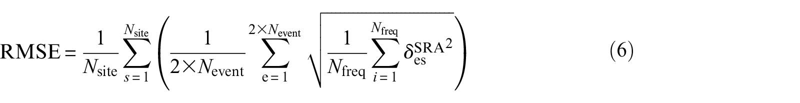
The most appropriate D_mul and ${\sigma }_{\ln V_S}$ , assumed to remove the intrinsic 1D-SRA error component $(\delta 1{\mathrm{D}}_s^{\mathrm{SRA}})$ , is selected using data from 1D-like sites. Such a D_mul- ${\sigma }_{\ln V_S}$ pair is found by minimizing the RMSE or “L2 error,” defined as follows:

$$\begin{array}{c}\multicolumn{1}{c}{\mathrm{RMSE}=\frac{1}{N_{\mathrm{site}}}\sum _{s=1}^{N_{\mathrm{site}}}\left(\frac{1}{2\times N_{\mathrm{event}}}\sum _{\mathrm{e}=1}^{2\times N_{\mathrm{event}}}\sqrt{\frac{1}{N_{\mathrm{freq}}}\sum _{i=1}^{N_{\mathrm{freq}}}{\delta }_{\mathrm{es}}^{{\mathrm{SRA}}^2}}\right)}\end{array}$$

(6)

where $N_{\mathrm{freq}}$ , $N_{\mathrm{event}}$ , and $N_{\mathrm{site}}$ are the number of frequencies, the number of earthquake events (Table 2), and the number of sites available in the 1D-like site database (N_site = 39), respectively. The residual ${\delta }_{\mathrm{es}}^{\mathrm{SRA}}$ is computed using Equation 1, where $\mathrm{IM}$ corresponds to the single 1D SRA–based TF or AF for cases with no V_S randomization or the median TF or AF otherwise. The number of earthquake events is factored by 2 as both horizontal components of the ground motion records are used independently. The frequency is normalized by each site’s fundamental frequency $(f_0)$ from the theoretical TFs, such that overpredictions at the site’s fundamental mode align at a common value of $f/f_0=1$ . Only the normalized frequencies from 0.5 (i.e. half $f_0$ ) to 20 times $f_0$ , or the maximum usable frequency in the borehole or surface recording, are used. The L2 error is computed for 200 natural logarithmically spaced values (i.e. N_freq = 200) sampled from $f/f_0$  = 0.5–20 to allow for a fair comparison across multiple sites. Complementary to the L2 error, the errors in site response predictions are also quantified as the mean absolute error (MAE) or “L1 error,” defined as follows:

$$\mathrm{MAE}=\frac{1}{N_{\mathrm{site}}}\sum _{s=1}^{N_{\mathrm{site}}}\left[\frac{1}{2\times N_{\mathrm{event}}}\sum _{\mathrm{e}=1}^{2\times N_{\mathrm{event}}}\left(\frac{1}{N_{\mathrm{freq}}}\sum _{i=1}^{N_{\mathrm{freq}}}\left|{\delta }_{\mathrm{es}}^{\mathrm{SRA}}\right|\right)\right]$$

(7)

The L2 and L1 errors are computed from total residuals ${\delta }_{\mathrm{es}}^{\mathrm{SRA}}$ as opposed to bias-corrected residuals $({\delta }_{\mathrm{es}}^{\mathrm{SRA}}-c_{1\mathrm{D}}^{\mathrm{SRA}})$ . Results not included herein for brevity showed that using bias-corrected residuals in the minimization of the L2 and L1 errors leads to optimum D_mul values associated with significantly high $c_{1\mathrm{D}}^{\mathrm{SRA}}$ across frequencies, which is undesirable.

Results

Independent effects of D _mul and σ_{lnV s} on the seismic response

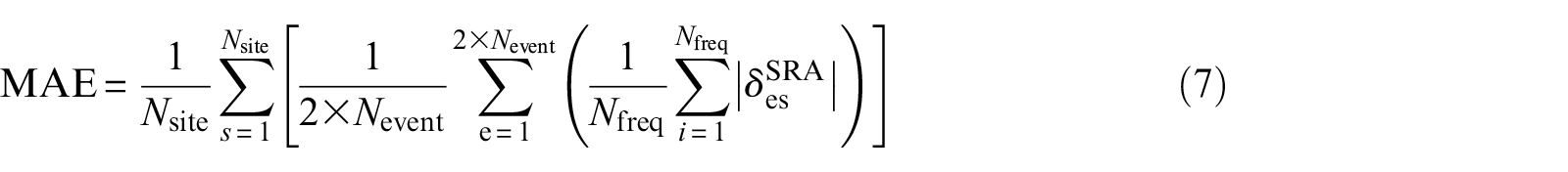
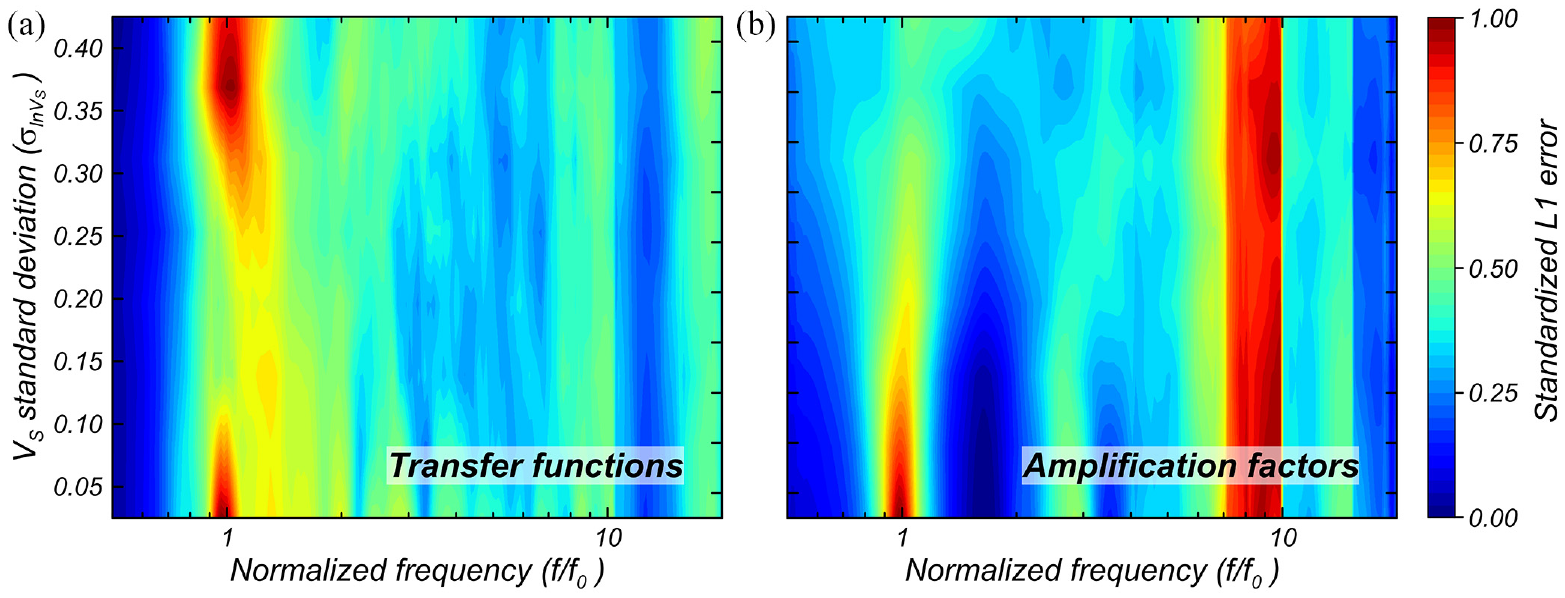
The L1 errors in TFs and AFs are calculated at individual $f/f_0$ and presented in Figures 8 and 9 for various D_mul and ${\sigma }_{\ln V_S}$ . These results are presented in terms of standardized errors, that is, L1 errors shifted and scaled to vary from 0 to 1 for better clarity. The sharp contrasts observed starting at $f/f_0\approx 5$ are partly due to the lower number of records available at high normalized frequencies (Figure 3b). These results indicate that increased damping and randomized V_S profiles can both improve 1D SRA predictions for 1D-like sites, but this improvement is not equally favorable across frequencies and neither for TFs and AFs simultaneously. For example, the predictions at the fundamental mode, $f/f_0=1$ , can be improved with D_mul > 6 for TFs and D_mul≈ 5 for AFs, but lower D_mul are more appropriate at higher frequencies for TFs and AFs. Similarly, Figure 9 suggests that using ${\sigma }_{\ln V_S}\approx 0.2$ and ${\sigma }_{\ln V_S}\approx 0.35$ can improve the predictions in TFs and AFs at $f/f_0=1$ , respectively, but lower ${\sigma }_{\ln V_S}$ are more appropriate at other $f/f_0$ . Based on these results, 1D SRAs with frequency-dependent damping are expected to be better suited to accurately estimate site response, as suggested in previous studies focused on nonlinear 1D SRAs (Assimaki and Kausel, 2002; Huang et al., 2020; Kausel and Assimaki, 2002; Kuo et al., 2021; Meite et al., 2020; Yoshida et al., 2002). Finally, the L1 error patterns for TFs are narrower, whereas they are broader for AFs. This is due to the wider range of frequencies that affects the response of a single degree of freedom oscillator with a given frequency in AFs (Bora et al., 2016), whereas TFs vary more independently, although with some inter-frequency correlation (e.g. Bayless and Abrahamson, 2019).

Figure 8.

Standardized L1 error in (a) transfer functions and (b) amplification factors across normalized frequencies $(f/f_0)$ for various damping multipliers (D_mul).

Figure 9.

Standardized L1 error in (a) transfer functions and (b) amplification factors across normalized frequencies $(f/f_0)$ for various V_S standard deviations $({\sigma }_{\ln V_S})$ for V_S randomization.

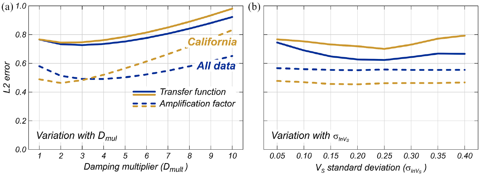
The L2 errors in TFs and AFs resulting from the independent use of D_mul and ${\sigma }_{\ln V_S}$ are presented in Figure 10 (darker lines labeled as “All data”), and a summary table for key D_mul- ${\sigma }_{\ln V_S}$ combinations in Supplemental Appendix E. There is a stronger effect of D_mul on TFs and AFs compared to ${\sigma }_{\ln V_S}$ . Overall, an initial reduction of the L2 with higher D_mul and ${\sigma }_{\ln V_S}$ values is observed, followed by an increase in L2 error starting at D_mul≈ 3, and ${\sigma }_{\ln V_S}\approx 0.25$ . The minor contribution of ${\sigma }_{\ln V_S}$ on the reduction of residual variability in AFs presented as L2 errors is likely due to the averaging effect of using data from multiple sites, ground motion recordings, and frequencies. At a specific site, the influence of ${\sigma }_{\ln V_S}$ on AFs, even though less pronounced compared to TFs, is not negligible (e.g. Figure 6c and d). Based on Figure 10, 1D SRA predictions could be improved by D_mul≈ 3 and no V_S randomization, or V_S randomization with ${\sigma }_{\ln V_S}=0.25$ and D_mul = 1. A D_mul = 3 is consistent with results by Tao and Rathje (2019), who estimated D_mul based on the variation of measured values of $\kappa$ at borehole array sites. A ${\sigma }_{\ln V_S}=0.2-0.3$ is consistent with findings by Pretell et al. (2022a), who compared results from 2D SRAs and 1D SRAs with V_S randomization to identify the most appropriate ${\sigma }_{\ln V_S}$ to capture the effects of V_S spatial variability of soils on the site response.

Figure 10.

Variation of L2 error with damping multiplier (D_mul) and V_S standard deviation $({\sigma }_{\ln V_S})$ for V_S randomization. Results labeled as “All data” based on the data from all the 39 1D-like sites from Japan and the United States, and results labeled as “California” based on the data from six 1D-like sites from California.

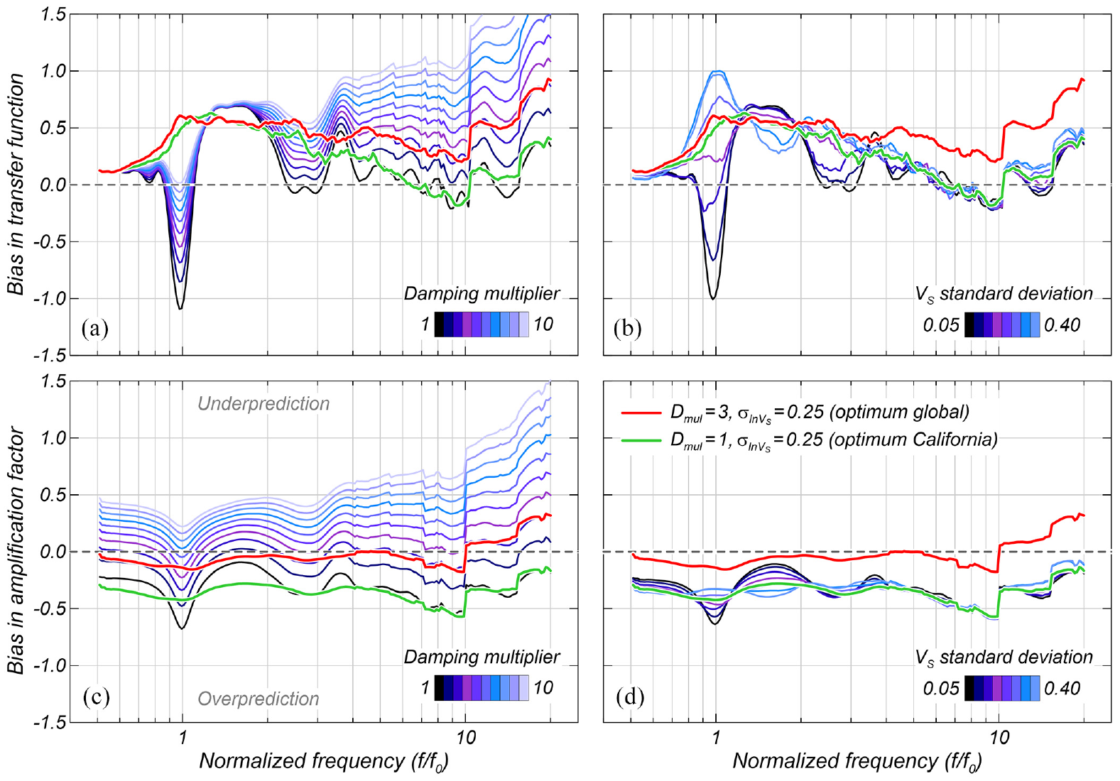
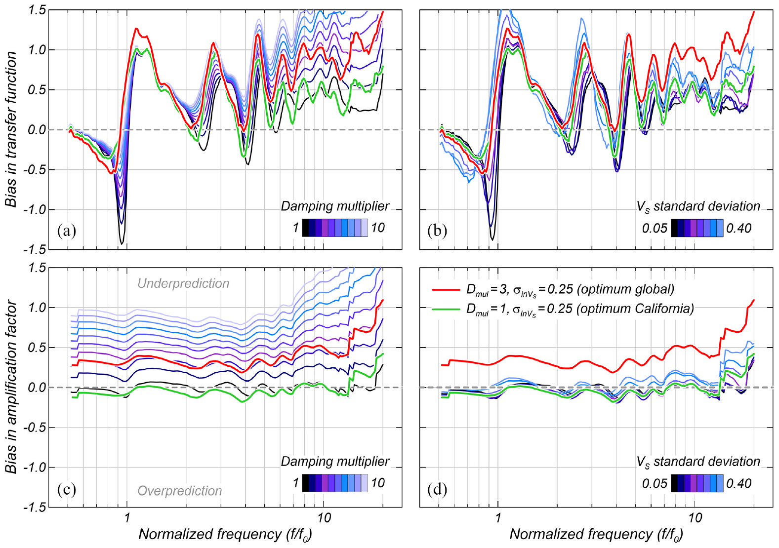
The independent effects of various D_mul and ${\sigma }_{\ln V_S}$ on the bias in TFs and AFs are presented in Figure 11. As previously observed, increases in D_mul lead to a reduction of the TF amplitudes that affects more strongly the high-frequency range, thus leading to a higher bias at high $f/f_0$ (Figure 11a and c). Importantly, the bias in TF at high $f/f_0$ values for D_mul = 1 is low, whereas a low bias in TF at $f/f_0=1$ is achieved with D_mul≈ 8 (Figure 11a). The variability of bias with ${\sigma }_{\ln V_S}$ mostly affects the low-frequency range, around $f/f_0=1$ (Figure 11b and d). Again, the variation of AF amplitudes is smoother compared to TFs.

Figure 11.

Bias in 1D site response estimates for 1D-like sites $(c_{1\mathrm{D}}^{\mathrm{SRA}})$ : (a) bias in transfer functions (TFs) for various damping multipliers (D_mul). (b) Bias in TFs for various V_S standard deviations $({\sigma }_{\ln V_S})$ . (c) Bias in amplification factors (AFs) for various D_mul. (d) Bias in AFs for various ${\sigma }_{\ln V_S}$ values.

Combined effect of D _mul and σ_{lnV s} on the seismic response

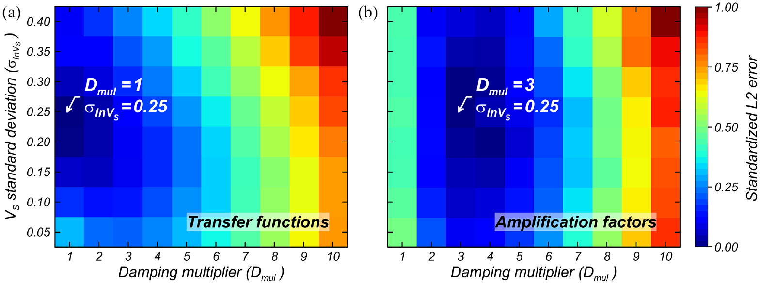
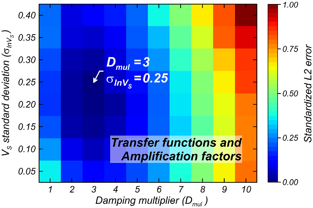
The previous section shows the independent impact of D_mul and ${\sigma }_{\ln V_S}$ on site response predictions in terms of TFs and AFs. Here, the combined effect of D_mul and ${\sigma }_{\ln V_S}$ is investigated by conducting SRAs with various D_mul- ${\sigma }_{\ln V_S}$ combinations and comparing the results against observations. The L2 errors in TFs and AFs are presented in Figure 12a and b, respectively, and their combined effect computed as the standardized averaged L2 error is presented in Figure 13. The 1D SRA bias associated with the most appropriate D_mul- ${\sigma }_{\ln V_S}$ trial is compared in Figure 11 against the bias resulting from scenarios with either D_mul or ${\sigma }_{\ln V_S}$ alone.

Figure 12.

Standardized L2 error for combinations of damping multiplier (D_mul) and V_S standard deviation $({\sigma }_{\ln V_S})$ for V_S randomization. (a) Standardized L2 error in transfer functions (TFs). (b) Standardized L2 error in amplification factors (AFs). Minimum standardized L2 error in TFs for D_mul = 1, and ${\sigma }_{\ln V_S}=0.25$ , and minimum standardized L2 error in AFs for D_mul = 3 and ${\sigma }_{\ln V_S}=0.25$ .

Figure 13.

Standardized averaged L2 errors in transfer functions (Figure 11a) and amplification factors (Figure 11b) for combinations of damping multiplier (D_mul) and V_S standard deviation $({\sigma }_{\ln V_S})$ for V_S randomization. Minimum standardized L2 error for D_mul = 3 and ${\sigma }_{\ln V_S}=0.25$ .

Results from the analyses indicate that a different combination of D_mul and ${\sigma }_{\ln V_S}$ is required to improve predictions for TFs and AFs. A ${\sigma }_{\ln V_S}=0.25$ leads to the minimum L2 error in TFs and no D_mul is needed (Figure 12a). Meanwhile, a ${\mathrm{\sigma }}_{\ln {\mathrm{V}}_{\mathrm{S}}}\approx$ 0.2–0.3 and a D_mul≈ 3–4 both lead to the lowest L2 error in AFs (Figure 12b). Overall, considering that TFs and AFs are equally important, the combination D_mul = 3 and ${\sigma }_{\ln V_S}=0.25$ leads to most appropriate site response predictions (Figure 13). Therefore, 1D SRAs conducted with a D_mul = 3 and randomized V_S profiles generated using the model by Toro with ${\sigma }_{\ln V_S}=0.25$ lead to (1) removing the intrinsic 1D SRA error $1{\mathrm{D}}_s^{\mathrm{SRA}}$ , and (2) the lowest variance in site response residuals. The removed $\delta 1{\mathrm{D}}_s^{\mathrm{SRA}}$ is the difference between the $c_{1\mathrm{D}}^{\mathrm{SRA}}$ corresponding to D_mul = 3 with ${\sigma }_{\ln V_S}=0.25$ , and the $c_{1\mathrm{D}}^{\mathrm{SRA}}$ corresponding to D_mul = 1 with no randomization (Figure 11). A similar D_mul- ${\sigma }_{\ln V_S}$ pair is obtained if the L1 error is considered as the decision metric instead of the L2 error (Supplemental Appendix F). For sites in the United States, damping profiles based on Darendeli (2001) with D_mul = 3 are similar or slightly higher in the top 10 m to those obtained based on the commonly used correlation with Q, Model 1 by Campbell (2009), but consistently lower at deeper locations.

As previously mentioned, the selection of the D_mul- ${\sigma }_{\ln V_S}$ pair focuses on minimizing the variance in residuals and improving site response predictions across frequencies on average, as opposed to reducing the systematic bias $c_{1\mathrm{D}}^{\mathrm{SRA}}$ . Figure 11 shows that as D_mul = 3 and ${\sigma }_{\ln V_S}=0.25$ leads to an overall reduction in $c_{1\mathrm{D}}^{\mathrm{SRA}}$ , but there is an increase of it at high frequencies for TFs. This increase results from a compromise between (1) selecting a single D_mul- ${\sigma }_{\ln V_S}$ pair that works for TFs and AFs across a wide range of frequencies and (2) using a different pair for TFs and AFs. This increase in bias must be addressed by bias-correcting site response predictions, as explained in the companion paper.

Sensitivity of the results

The previous results are based on the comparisons of 1D SRA predictions against data from 39 1D-like sites from Japan and the United States, and damping profiles developed after Darendeli (2001) assuming PI = 0, f_load = 1 Hz, and K₀ = 0.5. In this section, the regional differences between data from sites in California and Japan, and the effect of damping variables on the resulting D_mul- ${\sigma }_{\ln V_S}$ recommendation are investigated.

Regional differences

The selection of the most appropriate D_mul and ${\sigma }_{\ln V_S}$ leading to improved site response predictions of TFs and AFs is based on comparisons against data from six sites in California, one site in Alaska, and 32 sites in Japan. In this section, regional differences in the most appropriate D_mul- ${\sigma }_{\ln V_S}$ and the resulting $c_{1\mathrm{D}}^{\mathrm{SRA}}$ are investigated for California and Japan.

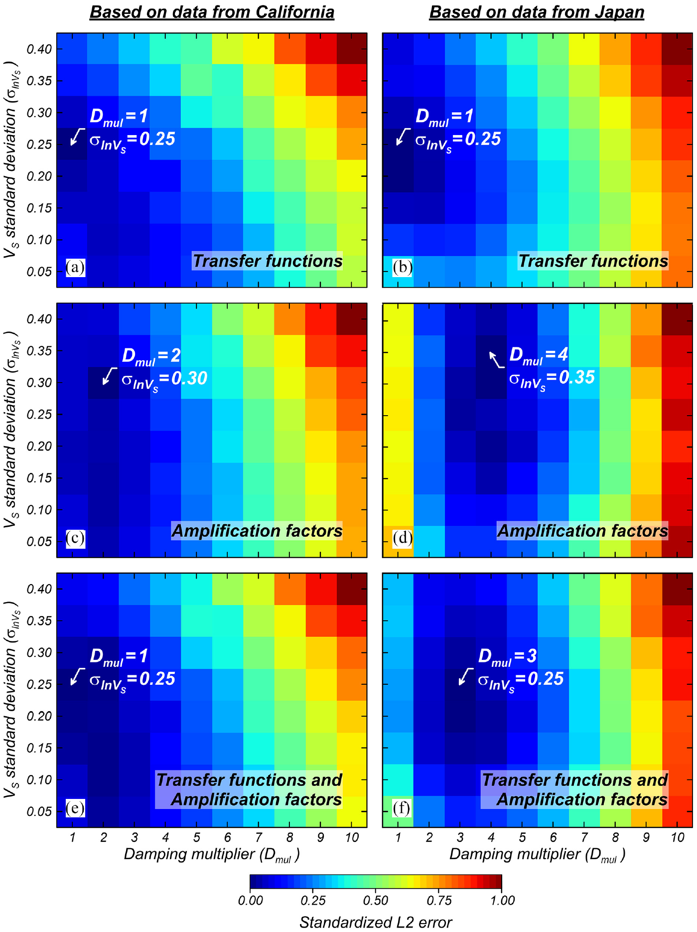
The most appropriate D_mul and ${\sigma }_{\ln V_S}$ to reduce the L2 error in TFs are the same for California and Japan (D_mul = 1 and ${\sigma }_{\ln V_S}=0.25$ ). However, differences are found in the case of AFs. Figure 14 shows the standardized L2 errors for TFs (a and b), AFs (c and d), and the average between the two (e and f). Figure 14c and d indicate that higher D_mul and ${\sigma }_{\ln V_S}$ are required to improve predictions in AFs in Japan. In particular, there is a clear need for a higher D_mul (also Figure 10) that is attributed to the overall more uniform amplification of seismic waves across frequencies observed in the data from Japan, with flatter TFs or median TFs with lower peak-to-trough ratios, for example, compare the observed TFs for Treasure Island and GIFH28 in Figure B1 (Supplemental Appendix B). The lower peak-to-trough ratio is indicative of a higher V_S spatial variability (e.g. de la Torre et al., 2021) and less compliance with 1D SRA assumptions. Such flatter response in TFs exacerbates the overamplification of AFs given the influence of the low-frequency waves across various oscillators’ frequencies. For instance, the TFs and AFs for SBSH06 in Figures B3 (Supplemental Appendix B) and C3 (Supplemental Appendix C), respectively, show how over- and underpredictions observed in TFs can turn into consistent overpredictions in AFs caused by the dominance of the overpredicted TF fundamental mode.

Figure 14.

Standardized L2 errors for various combinations of damping multipliers (D_mul) and V_S standard deviations $({\sigma }_{\ln V_S})$ for V_S randomization. (a), (c), and (e) Standardized L2 errors for sites in California. (b), (d) and (f) Standardized L2 errors for sites in Japan.

The appropriate D_mul- ${\sigma }_{\ln V_S}$ combination for TFs and AFs are D_mul = 1 and ${\sigma }_{\ln V_S}=0.25$ for California, and D_mul = 3 and ${\sigma }_{\ln V_S}=0.25$ for Japan (Figure 14). The latter is also the global recommendation based on all 39 1D-like sites (Figure 13). The $c_{1\mathrm{D}}^{\mathrm{SRA}}$ for California are shown in Figure 15, whereas the corresponding ones for Japan are very similar to the global estimates in Figure 11 and thus not presented. Figure 15 shows that SRAs for California generally underpredict the seismic response, consistent with previous studies (e.g. Stewart and Afshari, 2021). The observed differences indicate potential for improving site response predictions for regions that share similar features affecting site response (e.g. topography, subsurface conditions, soil deposition). However, the data available for California (Table 2) do not currently allow for region-specific recommendations of D_mul, ${\sigma }_{\ln V_S}$ , or the terms in Equation 5.

Figure 15.

Bias in 1D site response estimates for 1D-like sites $(c_{1\mathrm{D}}^{\mathrm{SRA}})$ in California. (a) Bias in transfer functions (TFs) for various damping multipliers (D_mul). (b) Bias in TFs for various V_S standard deviations $({\sigma }_{\ln V_S})$ . (c) Bias in amplification factors (AFs) for various D_mul. (d) Bias in AFs for various ${\sigma }_{\ln V_S}$ .

Effect of small-strain damping parameters

From the previously discussed evaluation, SRAs conducted with D_mul = 3 and randomized V_S profiles generated using ${\sigma }_{\ln V_S}=0.25$ lead to improved site response predictions. In this study, D_mul is applied to damping profiles developed after Darendeli (2001) assuming PI = 0, f_load = 1 Hz, and K₀ = 0.5, hereafter referred to as “default parameters” yielding the baseline damping (D^baseline). These parameters must be used when following the proposed approach; nevertheless, it is worth evaluating the effect of using different values to calculate the damping profiles. Henceforth, if parameters other than the default ones are used, the resulting damping is denominated D^{site-specific}. The overconsolidation ratio (OCR) has an effect when PI is higher than 0, thus it is also considered in this evaluation. The effect of any given parameter on the ultimate D_mul is quantified through the damping scaling factor (D_SF):

$$D_{\mathrm{SF}}=\frac{D^{\mathrm{site}\mathrm{-}\mathrm{specific}}}{D^{\mathrm{baseline}}}$$

(8)

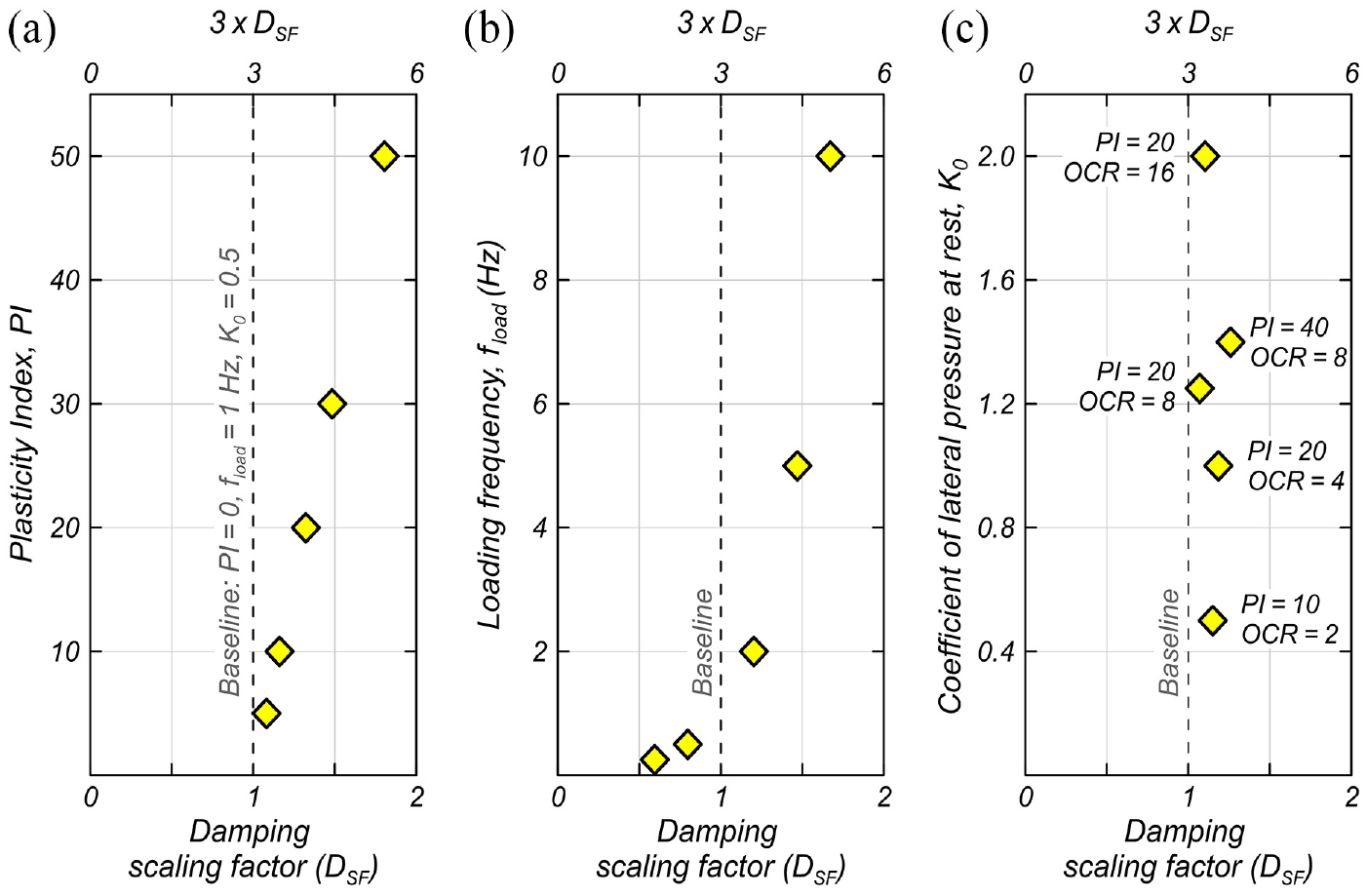
Different scenarios are considered to evaluate the effect of the Darendeli model parameters on the resulting D_SF. The effect of these parameters on the damping values are studied at a single arbitrary depth, but the D_SF is the same at any depth of a given profile. The results are presented in Figure 16 as D_SF and the corresponding $3\times D_{\mathrm{SF}}$ , that is, the impact on the damping resulting after applying D_mul = 3. These scenarios include results for various PI (Figure 16a), f_load (Figure 16b), and K₀ (Figure 16c). For the evaluation of K₀, various geotechnically consistent scenarios for OCR and PI are considered based on the data reported by Brooker and Ireland (1965) and Mayne and Kulhawy (1982).

Figure 16.

Effect of various parameters of the damping model by Darendeli (2001) on damping multiplier (D_mul). (a) Effect of plasticity index (PI). (b) Effect of loading frequency (f_load). (c) Effect of coefficient of lateral pressure at rest (K₀) and overconsolidation ratio (OCR).

Unsurprisingly, results from the parametric evaluation indicate that PI and f_load have an important effect on the D_mul, whereas K₀ leads to milder variations in D_mul. These findings are consistent with previous studies on clayey soils (e.g. Vucetic and Dobry, 1991). Variations of PI, OCR, f_load, and K₀ lead to D_SF values from 0.3 to 1.8, and thus $3\times D_{\mathrm{SF}}$ from 0.9 to 5.4. This means that applying a D_mul = 3 on damping profiles developed using values that differ from the recommended in this study can excessively increase damping (Figure 16), and lead to higher L2 errors (e.g. Figure 13 for D_mul = 3–5). The ultimate impact on TFs and AFs might be milder as not all layers in a given damping profile are likely to simultaneously differ from the default parameters. Nevertheless, it is recommended that the default parameters (PI = 0, f_load = 1 Hz, and K₀ = 0.5) be used in all cases when estimating the seismic site response following the proposed approach. Engineering problems involving materials that significantly deviate from the assumed values are expected to require analyses more advanced than 1D SRAs.

Conclusions

An approach is developed for improving site response predictions using one-dimensional site response analyses (1D SRAs). This approach combines damping multipliers (D_mul), and randomized shear-wave velocity (V_S) profiles with a V_S standard deviation ${\sigma }_{\ln V_S}$ , where D_mul and ${\sigma }_{\ln V_S}$ are calibrated based on the data from borehole array sites. This article discussed (1) the approach and framework for quantifying site response residuals and (2) the selection of the most appropriate D_mul- ${\sigma }_{\ln V_S}$ combination by comparing observed and theoretical transfer functions (TFs) and amplification factors (AFs) from sites relatively compatible with 1D SRA assumptions, denominated 1D-like sites. The companion paper discusses the use of D_mul and ${\sigma }_{\ln V_S}$ in forward predictions of site response for the more commonly encountered 3D-like sites and addresses the underprediction of high-frequency TF amplitudes caused by increasing the small-strain damping.

The results indicate that using a D_mul = 3 and ${\sigma }_{\ln V_S}=0.25$ leads to an overall minimum root mean square error (RMSE) in site response predictions. However, different values are obtained if the focus is placed on TFs or AFs separately or the available data are separated by region. A lower D_mul = 1 is required if TFs are the only metric of interest, and D_mul = 2 and 4 are, respectively, required for AFs for California and Japan when analyzed independently. The higher D_mul values required for AFs compared to TFs result from the wide range of ground motion frequencies affecting the spectral ordinates of a single-degree-of-freedom oscillator (Bora et al., 2016), and thus the AFs. The factor making a difference between D_mul for AFs in California and Japan is similar. The ground motions from the sites in Japan present a more uniform and generally higher amplification of waves across frequencies, suggested by flatter TF shapes (Supplemental Appendix B). These characteristics observed in TFs turn into larger contributions to the oscillators’ spectral ordinates and thus AF amplitudes (Supplemental Appendix C).

The analyses showed that the effects of D_mul and ${\sigma }_{\ln V_S}$ on the predicted TFs and AFs vary with frequency, and thus any D_mul- ${\sigma }_{\ln V_S}$ combination does not lead to a uniform reduction of the RMSE across frequencies. This suggests that frequency-dependent SRAs are better suited for site response predictions, which is consistent with findings from studies using nonlinear SRAs (Assimaki and Kausel, 2002; Kausel and Assimaki, 2002). Frequency-dependent SRAs have yet to make their way into practice.

A total of 39 1D-like sites from a database of 534 borehole array sites were identified based on the alignment of peaks and troughs of the median observed and the theoretical TFs measured using Pearson’s correlation coefficient, followed by a visual screening. The results indicate that only 39 of the 534 sites can be considered as 1D-like, which represents about 7% of the database. It is unclear whether the calibrated D_mul = 3 and ${\sigma }_{\ln V_S}=0.25$ would change with larger data sets of 1D-like sites, but it is expected that these recommendations will be revised as ground motion databases become larger. Similarly, the number of sites and ground motion recordings from California do not allow for providing region-specific recommendations, but there is potential for doing so as more data become available.

The D_mul and ${\sigma }_{\ln V_S}$ were estimated considering damping profiles after Darendeli (2001), and randomized V_S profiles generated using the V_S model by Toro (1995), without prior layer discretization. Therefore, following the proposed approach involves using these models and corresponding assumed parameters. The Darendeli model is used assuming a plasticity index (PI) = 0, a load frequency (f_load) = 1 Hz, and a coefficient of lateral pressure at rest (K₀) = 0.5. Using site-specific values that differ from these assumptions might lead to damping values higher by a factor of 2. It is expected that engineering problems involving soils that significantly deviate from the assumed values would require analyses more advanced than 1D SRAs. The V_S model by Toro is used with ${\sigma }_{\ln V_S}=0.25$ and the other parameters recommended for sites with V_S30 = 180–360 m/s, which are very similar to those for sites with V_S30 = 360–760 m/s, thus covering a wide range of V_S30.

The proposed approach focuses on linear elastic SRAs, the framework can be extended to nonlinear site response applications. The extension to equivalent linear 1D SRAs could involve using damping curves (e.g. Seed and Idriss, 1970) increased by an amount equivalent to the difference between the recommended and default laboratory-based damping, as opposed to D_mul applied to the entire damping curve. Alternatively, the low-strain tail of the damping curves could be scaled up (e.g. Kaklamanos et al., 2020). Further research needs to be conducted on the application of the proposed approach for equivalent linear and nonlinear 1D SRAs.

Supplemental Material

sj-pdf-1-eqs-10.1177_87552930231173445 – Supplemental material for A borehole array data–based approach for conducting 1D site response analyses I: Damping and VS randomization

Supplemental material, sj-pdf-1-eqs-10.1177_87552930231173445 for A borehole array data–based approach for conducting 1D site response analyses I: Damping and VS randomization by Renmin Pretell, Norman A Abrahamson and Katerina Ziotopoulou in Earthquake Spectra

Supplemental Material

sj-pdf-2-eqs-10.1177_87552930231173445 – Supplemental material for A borehole array data–based approach for conducting 1D site response analyses I: Damping and VS randomization

Supplemental material, sj-pdf-2-eqs-10.1177_87552930231173445 for A borehole array data–based approach for conducting 1D site response analyses I: Damping and VS randomization by Renmin Pretell, Norman A Abrahamson and Katerina Ziotopoulou in Earthquake Spectra

Supplemental Material

sj-pdf-3-eqs-10.1177_87552930231173445 – Supplemental material for A borehole array data–based approach for conducting 1D site response analyses I: Damping and VS randomization

Supplemental material, sj-pdf-3-eqs-10.1177_87552930231173445 for A borehole array data–based approach for conducting 1D site response analyses I: Damping and VS randomization by Renmin Pretell, Norman A Abrahamson and Katerina Ziotopoulou in Earthquake Spectra

Supplemental Material

sj-pdf-4-eqs-10.1177_87552930231173445 – Supplemental material for A borehole array data–based approach for conducting 1D site response analyses I: Damping and VS randomization

Supplemental material, sj-pdf-4-eqs-10.1177_87552930231173445 for A borehole array data–based approach for conducting 1D site response analyses I: Damping and VS randomization by Renmin Pretell, Norman A Abrahamson and Katerina Ziotopoulou in Earthquake Spectra

Supplemental Material

sj-pdf-5-eqs-10.1177_87552930231173445 – Supplemental material for A borehole array data–based approach for conducting 1D site response analyses I: Damping and VS randomization

Supplemental material, sj-pdf-5-eqs-10.1177_87552930231173445 for A borehole array data–based approach for conducting 1D site response analyses I: Damping and VS randomization by Renmin Pretell, Norman A Abrahamson and Katerina Ziotopoulou in Earthquake Spectra

Supplemental Material

sj-pdf-6-eqs-10.1177_87552930231173445 – Supplemental material for A borehole array data–based approach for conducting 1D site response analyses I: Damping and VS randomization

Supplemental material, sj-pdf-6-eqs-10.1177_87552930231173445 for A borehole array data–based approach for conducting 1D site response analyses I: Damping and VS randomization by Renmin Pretell, Norman A Abrahamson and Katerina Ziotopoulou in Earthquake Spectra