Seismic fragility of bridges: An approach coupling multiple-stripe analysis and Gaussian mixture for multicomponent structures

Abstract

An approach is developed to build multivariate probabilistic seismic demand models (PSDMs) of multicomponent structures based on the coupling of multiple-stripe analysis and Gaussian mixture models. The proposed methodology is eminently flexible in terms of adopted assumptions, and a classic highway bridge in Eastern Canada is used to present an application of the new approach and to investigate its impact on seismic fragility analysis. Traditional PSDM methods employ lognormal distribution and linear correlation between pairs of components to fit the seismic response data, which may lead to poor statistical modeling. Using ground motion records rigorously selected for the investigated site, data are generated via response history analysis, and appropriate statistical tests are then performed to show that these hypotheses are not always valid on the response data of the case-study bridge. The clustering feature of the proposed methodology allows the construction of a multivariate PSDM with refined fitting to the correlated response data, introducing low bias into the fragility functions and mean annual frequency of violating damage states, which are crucial features for decision making in the context of performance-based seismic engineering.

Introduction

Performance-based earthquake engineering (PBEE) promotes the concept that designed structures are expected to perform according to predefined standards during probable earthquakes, including uncertainties inherent in the evaluation of the potential hazard and in the quantification of the structural response. Intermediate steps of a PBEE probabilistic framework may include the definition of a model that establishes the probabilistic relationship between an engineering demand parameter $(\mathrm{EDP})$ and the seismic intensity measure $(\mathrm{IM})$ . This model is known as a probabilistic seismic demand model (PSDM) and is widely employed in constructing analytical fragility functions, common tools for the assessment of seismic performance of structures (Mackie and Stojadinovic, 2003). In PBEE, performance criteria relate damage limit states to required structural functionality, and for multicomponent structures, such as highway bridges, damage limit states are formulated at two levels: component and system. Often, component-level damages are used to estimate repair actions and costs, while system-level performance from this combination of component damages often relates to outcomes such as lane closures, load, or speed restrictions (Kameshwar et al., 2020; Mackie and Stojadinovic, 2004; Nielson and DesRoches, 2007; Padgett and DesRoches, 2008; Siqueira et al., 2014a). Past studies proposed methodologies to develop PSDMs that consider the contribution of multiple critical components based on system reliability and acknowledging the existence of correlation between pairs of structural component responses (Gardoni et al., 2003; Lupoi et al., 2006); the framework proposed by Nielson and DesRoches (2007) has been broadly employed in analytical assessments of the seismic fragility of highway bridges since then (Padgett and DesRoches, 2008; Ramanathan et al., 2015; Siqueira et al., 2014a; Tavares et al., 2012; Zakeri et al., 2014).

Fragility functions are inherently uncertain quantities subject to numerous sources of both aleatory and epistemic uncertainty; one source is intrinsically related to the hypotheses adopted in the development of PSDMs, and significant bias may be introduced if imperfect modeling assumptions are adopted (Bakalis and Vamvatsikos, 2018; Der Kiureghian and Ditlevsen, 2009). A crucial step in the construction of a PSDM is the generation of structural response data with typical strategies including (1) cloud analysis (e.g. Mackie and Stojadinovic, 2003; Nielson and DesRoches, 2007; Padgett and DesRoches, 2008), (2) incremental dynamic analysis (IDA) (Vamvatsikos and Cornell, 2002), and (3) multiple-stripe analysis (MSA) (Jalayer and Cornell, 2009). Each collection strategy presents advantages in terms of choice of record selection and scaling, practicality, and adopted hypotheses (Baker, 2015; Eads et al., 2013; Gehl et al., 2015; Mackie and Stojadinovic, 2005). Once demand data are gathered, a PSDM is traditionally built using simple techniques such as linear regression (when cloud analysis is used) or fitting parametric distributions—usually lognormal—if IDA or MSA is employed.

It is often assumed, for simplicity and tractability, that (1) demand follows a normal distribution in the logarithmic space (lognormality), (2) the variability of the demand is constant and independent of the $\mathrm{IM}$ level (homoscedasticity), and (3) component responses are linearly correlated (linear dependence). The impacts of homoscedasticity on fragility are acknowledged, and alternatives to avoid it are the use of a data collection strategy that allows one to calculate the variation of dispersion (for instance, MSA or IDA) (Bakalis and Vamvatsikos, 2018; Simon and Vigh, 2016) or the adoption of piecewise linear regression when cloud analysis is chosen (Freddi et al., 2017; Mackie and Stojadinovic, 2003). Lognormality of seismic structural demand has been validated in some studies—usually using either single-degree-of-freedom or two-dimensional frame models (e.g. Aslani and Miranda, 2005; Decanini et al., 2003; Ibarra and Krawinkler, 2005; Shome, 1999)—and rejected as a general assumption by others—who considered more complex systems such as highway bridges (e.g. Karamlou and Bocchini, 2015; Mangalathu and Jeon, 2019). The bias propagated into fragility functions of bridge components due to the lack of fit of seismic response data to a lognormal distribution, however, was deemed generally negligible by Karamlou and Bocchini (2015), whereas Mangalathu and Jeon (2019) suggested that it had lead to low impact on the fragility median and larger effect on the fragility dispersion. With respect to the dependence between pairs of component responses, typical cloud analysis (e.g. Ghosh et al., 2014; Nielson and DesRoches, 2007) considers the entire dataset of observed demands to estimate linear correlation coefficients, assuming that the correlation of component responses is linear and independent of the seismic intensity level. Still in the scope of cloud analysis, Zhou and Li (2019) proposed the use of vine copulas to model nonlinear dependence between bridge components and suggested that the assumption of linear dependence may have biased the built seismic fragility functions for a two-span case-study bridge. In contrast, Lupoi et al. (2006) had already investigated the importance of correlation between component responses in long multispan bridges and observed its strong dependence on the level of seismic intensity and on the number of response history analyses (RHAs).

Contemporary computational resources and data availability have also allowed the use of alternative machine learning techniques, applying supervised techniques for regression, for instance, polynomial response surfaces (Ghosh et al., 2014; Kameshwar and Padgett, 2014; Xie and DesRoches, 2019), artificial neural networks (Mangalathu et al., 2018), partial least square regression (Du and Padgett, 2020), and random forest (Mangalathu and Jeon, 2019), or unsupervised learning for density modeling, such as kernel density estimator (Karamlou and Bocchini, 2015). These learning techniques may employ parametric or nonparametric approaches to better model the observed seismic demand data. Although these approaches are more flexible, some of the resulting models still rely on unverified hypotheses (e.g. linear dependence).

One can thus conclude that there is still no consensus on the validity of traditional hypotheses for the construction of multivariate PSDMs or on their influence on seismic fragility of multicomponent structures. This study proposes a new strategy of probabilistic seismic demand modeling based on MSA and Gaussian mixture (GM) models that relaxes the traditional hypotheses adopted by current strategies by exploiting the ability to better capture the record-to-record variability of MSA and the flexibility in density modeling provided by parametric unsupervised learning techniques such as finite mixture models. The goal is thus twofold: (1) first to test whether bias is propagated into fragility analysis due to limitations of current hypotheses on the distribution and correlation of component seismic demands, and (2) second to provide an analytical tool for probabilistic seismic demand modeling in a structure-specific context for performance-based design or retrofit (where certain structures may violate traditional assumptions in demand modeling). The proposed model is leveraged for the construction of fragility curves and calculation of the mean annual frequency (MAF) of violating a damage state using a case-study continuous concrete-girder bridge in Eastern Canada. The case study is also used to further assess the validity of the assumptions on lognormality and linear dependence through appropriate goodness-of-fit tests and visual inspection of data. The impacts of these hypotheses on fragility and MAF of damage state violation are studied, and the advantages of the proposed method are highlighted.

Proposed methodology

The method proposed in this article for probabilistic seismic demand modeling is called MSA-GM, as it couples MSA and GM models to define joint distributions over seismic component demand at IM levels of interest. Contrary to cloud analysis (in which data are generated for different $\mathrm{IM}$ levels providing a cloud of points), MSA organizes demand data at a set of discrete $\mathrm{IM}$ levels (stripes), and this strategy allows better capturing locally, the record-to-record variability. Although it can be interpreted as a discrete version of IDA, MSA is preferred over IDA due to (1) the possibility to use different record sets for each seismic intensity level of interest, (2) limited scale factor, and (3) higher efficiency to account for seismic variability (i.e. fewer RHAs are required) (Baker, 2015; Eads et al., 2013; Luco and Bazzurro, 2007).

GM models are often employed as unsupervised machine learning tools on the task of clustering (i.e. to determine the number and the location of clusters in unlabeled datasets) or as a mathematical-based approach for density modeling of a wide variety of random phenomena (Bishop, 2006; McLachlan and Basford, 1988; McLachlan and Peel, 2000). In the present work, the latter is adopted to model the probability densities of seismic component demands by fitting finite mixtures of multivariate normal distributions to data in the logarithmic space at each stripe that are able to capture the interaction between components in a parametric form. A mathematical description of GM models is provided next along with the steps to build GM-based seismic demand models.

GM seismic demand model

A GM model is a probabilistic model that assumes all the data points are generated from a mixture of a finite number of Gaussian distributions with unknown parameters. The model is defined as the sum of $n_k$ multivariate normal probability density functions (PDFs), each weighted by a probability ${\pi }_k,\forall k=1,\dots ,n_k$ . Taking $\mathbf{X}$ as a multivariate random variable of an observed dataset $\mathbf{x}$ (e.g. the logarithm of the response of bridge components at a given seismic intensity level $\mathrm{EDP}|\mathrm{IM}$ ), the joint posterior PDF for a GM is thus defined by:

$$f(\mathbf{x}|\mathbf{\Psi })=\sum _{k=1}^{n_k}{\pi }_{k}f(\mathbf{x};{\mathbf{\mu }}_k,{\mathbf{\Sigma }}_k)$$

(1)

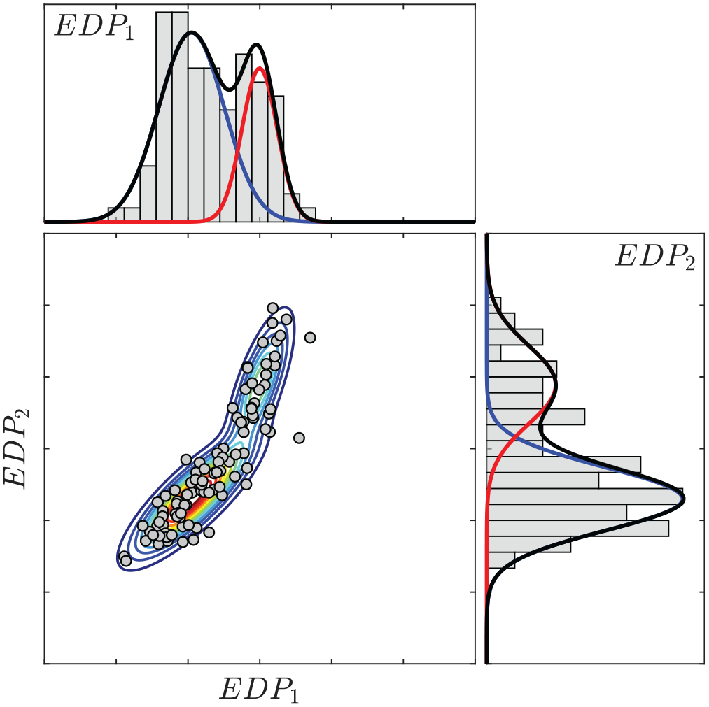
where $\mathbf{\Psi }=[{\mathbf{\pi }}^{\mathrm{T}},{\mathbf{\xi }}_1^{\mathrm{T}},\dots ,{\mathbf{\xi }}_{n_k}^{\mathrm{T}}{]}^{\mathrm{T}}$ is the vector that aggregates all the hyperparameters, being $\mathbf{\pi }=[{\pi }_1,\dots ,{\pi }_{n_k-1}{]}^{\mathrm{T}}$ the vector of mixture proportions; each vector ${\mathbf{\xi }}_k$ contains the hyperparameters related to the mean vector ${\mathbf{\mu }}_k$ and the covariance matrix ${\mathbf{\Sigma }}_k$ of the $k\mathrm{th}$ mixture cluster; ¹ and $f(\mathbf{x};{\mathbf{\mu }}_k,{\mathbf{\Sigma }}_k)$ is the PDF of a multivariate Gaussian with mean ${\mathbf{\mu }}_k$ and covariance ${\mathbf{\Sigma }}_k$ . Figure 1 exemplifies the simplicity of the concept by mixing two Gaussian distributions to bivariate data samples of $\mathbf{X}=[\mathrm{ED}{\mathrm{P}}_1,\mathrm{ED}{\mathrm{P}}_2]$ . This example illustrates, along with the histograms of the two random variables, the probability distribution functions of: (1) the first cluster (in blue), (2) the second cluster (in red), and (3) the resulting GM model (in black). The modeling of the correlation between the random variables $\mathrm{ED}{\mathrm{P}}_1$ and $\mathrm{ED}{\mathrm{P}}_2$ can also be appreciated by the contour plots of the PDF of the fitted GM presented along with the scattered data.

Figure 1.

Gaussian mixture model of bivariate data with two clusters.

The mean vector indicates the location of the center of each mixture cluster, while the covariance matrix incorporates information about the variance and correlation structures of the data. The complexity of a GM model depends on the number of clusters and the type of covariance structure adopted. Covariance matrices can be diagonal or full and shared or unshared. In the isotropic case, models employ diagonal-shared covariance, assuming a single diagonal covariance matrix for all clusters. Conversely, in the unrestricted case, the most complex GM model (in terms of number of hyperparameters per cluster) adopts a full-unshared covariance structure that fits a full covariance matrix for each cluster (McLachlan and Peel, 2000).

The first step to build a GM model is to learn the hyperparameters of the latent clusters that best fit the data; thus, the expectation-maximization (EM) algorithm is employed. This algorithm consists of an iterative approach that alternates between the expectation step, in which missing values are inferred given the estimated hyperparameters, and the maximization step, in which the hyperparameters are optimized given the inferred data (Murphy, 2012). Next, the most suitable number of mixture clusters must be chosen, and this model selection can be performed using information-theoretic criteria for a compromise between the fit and the complexity of the model (represented by the number of clusters and, hence, hyperparameters). In the context of density modeling, the Bayesian information criterion (BIC) is recommended over other information-criterion metrics in the selection of the number of clusters of a GM model, although excessively simple models can be obtained due to the use of finite observed samples and its heavy penalty on complexity (Bishop, 2006; Hastie et al., 2017; McLachlan and Peel, 2000). The BIC estimates the lack of fit through the negative log-likelihood and penalizes the model complexity to avoid overfitting:

$$\mathrm{BIC}=-2\ln (ℒ(\widehat{\mathbf{\Psi }}))+p\ln (n)$$

(2)

where $\mathcal{L}(\hat{\mathbf{\Psi }})$ is the likelihood of the data given the learned hyperparameters $\hat{\mathbf{\Psi }}$ , $p$ is the number of hyperparameters, and $n$ is the number of observations. The intent therefore is to pick a model that minimizes the criterion (McLachlan and Peel, 2000).

The construction of the MSA-GM seismic demand model starts by collecting the seismic demand data using the MSA. Hence, a suite of ground motions that well represents the seismicity of the site must be initially chosen, and Baker (2015) suggests using a conditional $\mathrm{IM}$ -based record selection approach, for instance, conditional spectrum (CS) (Baker, 2011; Jayaram et al., 2011) or generalized conditional intensity measure (GCIM) (Bradley, 2010, 2012a). RHAs are then performed with the selected records, and the seismic demand dataset $\mathrm{EDP}|\mathrm{IM}$ is generated. After the MSA step, the following steps are performed:

• Step 1. Select a covariance structure (e.g. full-unshared);

• Step 2. Learn the hyperparameters $\mathbf{\Psi }$ of a GM model with $n_k$ mixture clusters to model the demand data $\mathrm{EDP}$ at a given $\mathrm{IM}$ level by applying the EM algorithm;

• Step 3. Compute the BIC for the fitted GM model;

• Step 4. Repeat steps 2 and 3 for a set of number of clusters of interest $n_k=1,2,\dots ,n_{k,\max }$ ;

• Step 5. Select the model with the lowest $\mathrm{BIC}$ ;

• Step 6. Repeat steps 2 to 5 for all the $n_{\mathrm{IM}}$ levels of the IM;

• Step 7. Repeat steps 1 to 6 for different covariance structures and select the structure that minimizes the $\mathrm{BIC}$ (if applicable).

This formulation still assumes lognormality of seismic demand (the model is based on the mixture of Gaussians in the logarithmic space) and linear correlation between components within each mixture cluster. The formulation can be, however, multimodal, providing flexibility to the model in treating probability densities and linear correlation that can locally fit the dependence of observed data within each mixture cluster. Therefore, the models are able to draw samples of correlated seismic demand with good agreement to the data used in the learning process, as will be exemplified subsequently. The obtained seismic demand models are limited to generating samples of correlated component responses only for the $\mathrm{IM}$ levels at which they were trained.

Leveraging the MSA-GM approach for fragility analyses

The seismic fragility of a structure is the probability of violating a damage state $\mathrm{DS}$ (i.e. limit state exceedance) conditional on the occurrence of a seismic event with intensity $\mathrm{IM}=\mathrm{im}$ , that is, $\mathrm{Pr}(\mathrm{DS}|\mathrm{IM}=\mathrm{im})$ . Structures are composed of several components that can fail separately or at the same time during an extreme event. For instance, bridges are conventionally constituted by a deck, bearings, and supports (abutments and columns), and a holistic assessment of seismic vulnerability for the bridge must be made by combining the effects of the various critical structural elements (or components).

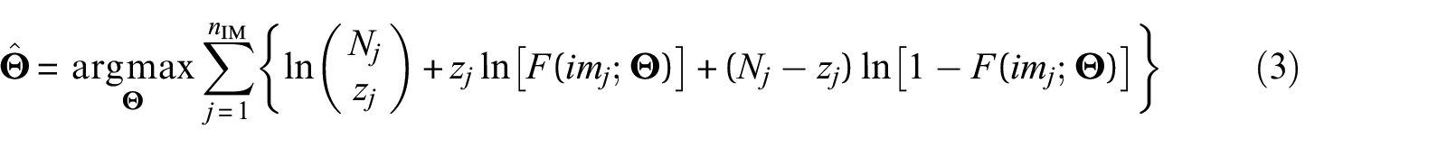
To account for the uncertainty in both demand and capacity in the fragility analysis, samples can be generated from the demand and capacity models (using Monte Carlo or Latin hypercube sampling). Using the MSA-GM seismic demand model, correlated component demand samples are drawn at each $\mathrm{IM}$ level (the same used in the construction of the PSDM). Demand and capacity samples are paired, and the violation of the damage state is verified when the demand is greater than the capacity. An efficient strategy for fragility curve fitting using results from MSA is described by Baker (2015), and the assumption that observing a damage state exceedance from each seismic ground motion is independent of the observations from other ground motions is here extrapolated for the generated samples. Thus, the probability of observing $z_j$ cases violating a damage state out of the total number of samples $N_j$ (on the stripe $\mathrm{IM}=i{m}_j$ ) is given by a binomial distribution in which $p_j$ is approximated by the fragility function, that is, $p_j\approx \mathrm{Pr}(\mathrm{DS}|\mathrm{IM}=i{m}_j)$ . Then, adopting the cumulative density function (CDF) of a parametric probability distribution to approximate the fragility $\mathrm{Pr}(\mathrm{DS}|\mathrm{IM}=\mathrm{im})=F(\mathrm{im};\mathbf{\Theta })$ with parameters $\mathbf{\Theta }$ , these parameters can be estimated by maximizing the log-likelihood using the maximum likelihood estimation (MLE) as in:

$$\hat{\mathbf{\Theta }}=\underset{\mathbf{\Theta }}{\arg \max }\sum _{j=1}^{n_{\mathrm{IM}}}\{\ln \left(\begin{array}{c}{N}_j\hfill \\ \multicolumn{1}{c}{z_j}\end{array}\right)+z_j\ln [F(i{m}_j;\mathbf{\Theta })]+(N_j-z_j)\ln [1-F(i{m}_j;\mathbf{\Theta })]\}$$

(3)

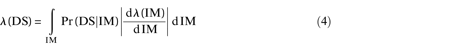
In addition, throughout its lifetime, a structure is potentially exposed to a range of ground motion intensities at a given site, as characterized by the site-specific seismic hazard curve. For a thorough analysis, the assessment of the annual risk can also be performed, which is measured here by the MAF of violating a specified damage state $\lambda (\mathrm{DS})$ . Given that the fragility function is defined for a certain damage state exceedance, this probability can be calculated by convolving the fragility with the hazard curve of the conditioning IM:

$$\lambda (\mathrm{DS})=\underset{\mathrm{IM}}{\int }\mathrm{Pr}(\mathrm{DS}|\mathrm{IM})\left|\frac{\mathrm{d}\lambda (\mathrm{IM})}{\mathrm{d}\mathrm{IM}}\right|\mathrm{d}\mathrm{IM}$$

(4)

where $\mathrm{d}\lambda (\mathrm{IM})/\mathrm{d}\mathrm{IM}$ is the derivative of the hazard curve with respect to the $\mathrm{IM}$ of interest (Bakalis and Vamvatsikos, 2018; Eads et al., 2013).

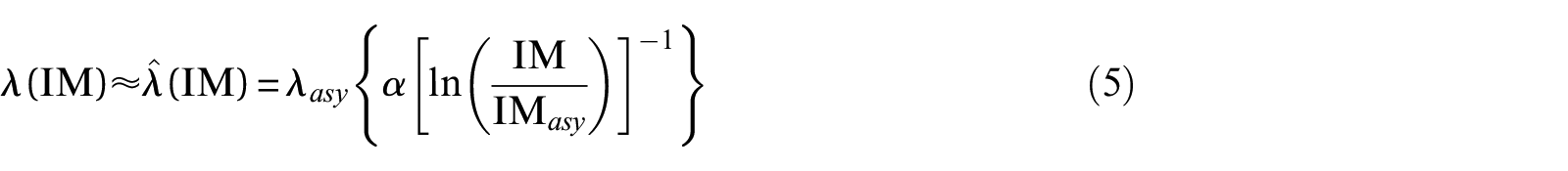
Annual risk calculations can be performed using the raw data provided by the seismic hazard curve although for certain sites the hazard data are sparse and significant interpolation between data points may be required. For instance, Bradley et al. (2007) proposed a hyperbolic model in the log-transformed space to fit the hazard curve to an analytical expression:

$$\lambda (\mathrm{IM})\approx \hat{\lambda }(\mathrm{IM})={\lambda }_{\mathrm{asy}}\left\{\alpha {\left[\ln \left(\frac{\mathrm{IM}}{\mathrm{I}{\mathrm{M}}_{\mathrm{asy}}}\right)\right]}^{-1}\right\}$$

(5)

where ${\lambda }_{\mathrm{asy}}$ , $\alpha$ , and $\mathrm{I}{\mathrm{M}}_{\mathrm{asy}}$ are the parameters to be estimated from minimizing the error between the data and the proposed curve (using, for example, least-squares minimization).

Case study: Chemin des Dalles bridge

As a classic multicomponent structural system, the Chemin des Dalles overpass, located in Quebec, Canada, is adopted to illustrate the proposed method. It is a $106.5\mathrm{m}$ long symmetric continuous concrete girder bridge with three equally spaced spans and a $13.2\mathrm{m}$ wide deck. The superstructure is composed of a $0.165\mathrm{m}$ depth deck and six prestressed concrete AASHTO type-V girders directly connected at the bents and supported by elastomeric bearings at the abutments. Pier bents are composed of three circular columns and square section cap beams, with a vertical clearance of $6.2\mathrm{m}$ . Bent columns are rigidly connected to the shallow foundations in the west bent and free for rotation in the east bent. The substructure also comprises seat-type abutments with wing walls supported by shallow foundations, with a $25.4\mathrm{mm}$ gap separating the deck from the abutment wing walls. This bridge was designed in 1975 and does not comply with current seismic design standards and detailing. It has been extensively studied and comprehensive data is available on the structural properties, capacity, site conditions, and numerical model (Roy et al., 2010; Siqueira et al., 2014b; Tavares et al., 2013; Zuluaga Rubio et al., 2019). Details on the numerical model, component capacities, and ground motion record selection are presented next.

Numerical model

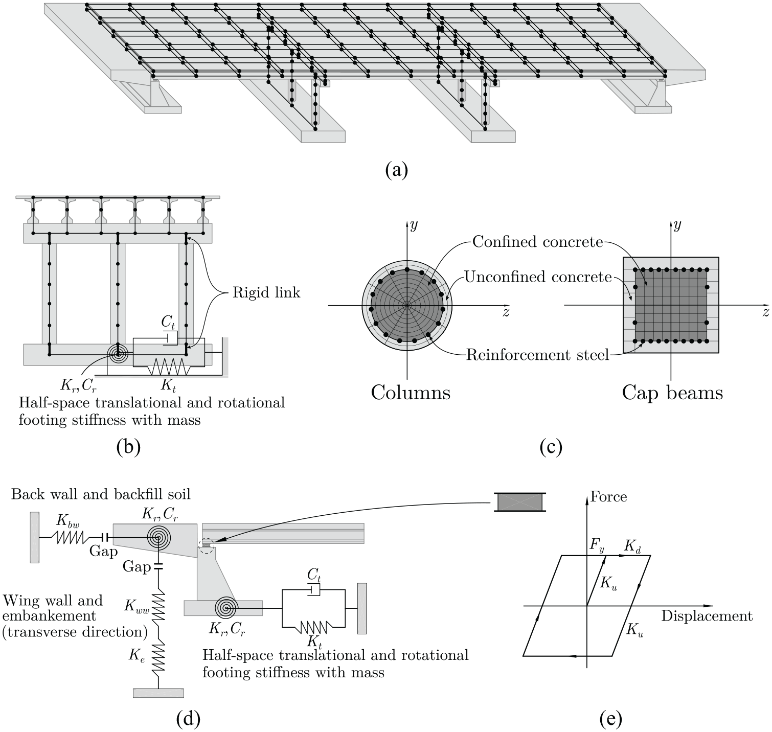
The three-dimensional finite element model originally built by Tavares et al. (2013) is revisited in this work. The model was created on the Open System for Earthquake Engineering Simulation (OpenSees) (McKenna et al., 2010), and it uses beam-column elements and zero-length elements to represent the behavior of this structural system and to capture the nonlinear behavior of critical structural components. Superstructure elements, including the concrete slab and girders, are defined as linear-elastic elements, while the substructure is constituted by the nonlinear elements. Bent columns and cap beams are modeled using force-based beam-column elements with their cross-sections discretized with fibers (Neuenhofer and Filippou, 1998). With the increase of the number of integration points within force-based elements, general improvement of both global and local responses is observed without excessive mesh refinement. Columns are discretized in five elements along their height with five Gauss-Lobatto integration points within each element. Concrete fibers are modeled with Concrete02 (Kent-Park) material while reinforcement layers are modeled using Steel02 (Giuffré-Menegotto-Pinto) uniaxial material. Confined concrete properties are calculated according to the formulation proposed by Légeron and Paultre (2003). To verify if lost of objectivity due to localization issues takes place (Coleman and Spacone, 2001; Scott and Fenves, 2006), the column analytical model is validated and calibrated against experimental data. Good agreement is observed from laboratory reversed cyclic-test results of an exact replica of the actual bridge column (Zuluaga Rubio et al., 2019). Strain-penetration effects at the intersection of columns and footings or cap beams are neglected, and the connection of columns to the cap beams and shallow foundation is modeled by rigid-link objects (Figure 2b). Soil–structure interaction is incorporated by adding elastic half-space spring-dashpot systems (using zero-length elements) and mass to the footing nodes (Canadian Standards Association, 2014; Clough and Penzien, 1975; Newmark and Rosenblueth, 1971; Rowe, 2001). Abutments are modeled as a series of elastic and elastic-gap zero-length elements to account for the back walls, wing walls, embankment and gap between the deck and abutments (Crouse et al., 1987; Mackie and Stojadinovic, 2003; Wilson, 1988; Wilson and Tan, 1990). Elastomeric bearings are also modeled with zero-length elements to behave as an elastic-perfectly plastic material (AASHTO, 2007). Lumped masses are defined for superstructure and substructure elements. Rayleigh damping corresponding to an average damping ratio of $1.5\%$ at the first and second vibration modes is adopted to perform RHA. A similar modeling approach has been adopted on the assessment of the seismic performance of bridges in Eastern Canada (Siqueira et al., 2014a, 2014c; Tavares et al., 2012). Finally, the numerical model is calibrated against in situ ambient vibration test results (vibration frequencies, mode shapes, and modal dampings) provided by Roy et al. (2010). An overview of the bridge model as well as some details on bents, columns, and abutments are illustrated in Figure 2. Further details on the numerical model and its calibration are found elsewhere (Siqueira et al., 2014b; Tavares et al. 2013).

Figure 2.

Numerical model of the case-study bridge: (a) overview, (b) bent elevation, (c) fiber sections, (d) abutment, and (e) material model for elastomeric bearings.

Damage states and capacity models

The damage states related to the seismic performance criteria defined in Section 4 of the Canadian highway bridge design code (CHBDC) CSA S6-14 (Canadian Standards Association, 2014) are adopted in this study for the assessment of the bridge’s fragility, namely, minimal, repairable, extensive, and probable replacement. These performance criteria indicate gradually progressive damage states that are similar to those established by HazUS (Federal Emergency Management Agency, 2015).

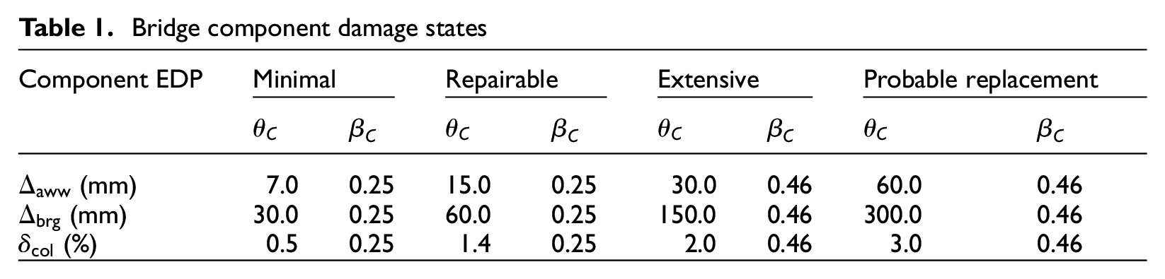
The case-study bridge includes three critical components: abutment wing walls, elastomeric bearings, and bent columns. Other structural components have shown negligible seismic fragility on multi-span continuous concrete girder bridges in Eastern Canada (Siqueira et al., 2014a; Tavares et al., 2012). The associated EDPs are the deformation on the wing walls and bearings ( ${\mathrm{\Delta }}_{\mathrm{aww}}$ and ${\mathrm{\Delta }}_{\mathrm{brg}}$ , respectively), and drift of fixed-base bent columns $({\delta }_{\mathrm{col}})$ ; all in the transverse direction (Siqueira et al., 2014b). Component capacities are assumed to follow lognormal distributions (Mangalathu and Jeon, 2019; Nielson and DesRoches, 2007), and their median $({\theta }_C)$ and dispersion $({\beta }_C)$ values for each damage state are presented in Table 1. The median capacities of columns follow the findings of Zuluaga Rubio et al. (2019) who established column damage states in accordance to the performance criteria of the CHBDC CSA S6-14 based on experimental tests, which included an exact replica of the actual bridge column. The median capacities of the other components were adapted by Tavares et al. (2013) for structures in Quebec based on the prescriptive damage states proposed by Choi et al. (2004). Dispersion values follow the recommendations given by Nielson (2005).

Table 1.

Bridge component damage states

Component $\mathrm{EDP}$	Minimal		Repairable		Extensive		Probable replacement
	${\theta }_C$	${\beta }_C$	${\theta }_C$	${\beta }_C$	${\theta }_C$	${\beta }_C$	${\theta }_C$	${\beta }_C$
${\mathrm{\Delta }}_{\mathrm{aww}}$ (mm)	7.0	0.25	15.0	0.25	30.0	0.46	60.0	0.46
${\mathrm{\Delta }}_{\mathrm{brg}}$ (mm)	30.0	0.25	60.0	0.25	150.0	0.46	300.0	0.46
${\delta }_{\mathrm{col}}$ (%)	0.5	0.25	1.4	0.25	2.0	0.46	3.0	0.46

Seismic hazard and record selection

Seismic ground motion record selection is performed using the GCIM approach (Bradley, 2010, 2012a) by adapting an algorithm with greed optimization (Baker and Lee, 2018; Jayaram et al., 2011) to include other $\mathrm{IMs}$ in addition to spectral acceleration. In the GCIM approach, a multivariate lognormal distribution of IMs is built conditioned on the occurrence of an earthquake event with a given intensity level (the conditioning IM). To build this conditional distribution, a conditioning $\mathrm{IM}$ must be chosen (referred as $\mathrm{I}{\mathrm{M}}_j$ ) along with the concomitant conditioned $\mathrm{IMs}$ (referred as $\mathrm{I}{\mathrm{M}}_i$ ). The conditional multivariate lognormal distribution $\mathrm{LN}(\mathrm{IM}|\mathrm{I}{\mathrm{M}}_j)$ is then used as target for the record selection, in which $\mathrm{IM}$ is the vector of conditioned IMs $\mathrm{I}{\mathrm{M}}_i$ . The choice of the seismic IMs depends on the availability of ground motion models (GMM) and correlation models between pairs of $\mathrm{IMs}$ at the investigated site.

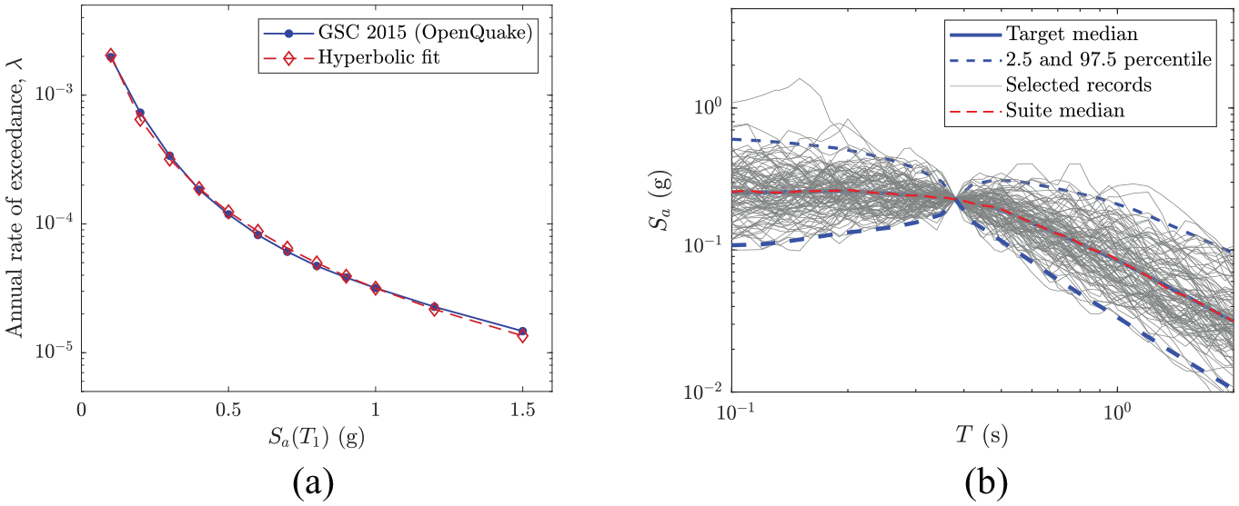
First, a probabilistic seismic hazard analysis (PSHA) is performed at the bridge site using the software OpenQuake (Silva et al., 2014) to identify expected earthquake scenarios. The most recent GMMs for Eastern Canada (Atkinson and Adams, 2013) are employed along with the source clusters and logic tree weights considered by the Geological Survey of Canada (Halchuk et al., 2014). These GMMs and logic tree models are the same used in the construction of the Canadian seismic hazard maps adopted by the 2015 edition of the National Building Code of Canada (Canadian Commission on Building and Fire Codes and National Research Council Canada, 2015). The resulting hazard curve is presented in Figure 3a, and the hyperbolic curve fitted to the hazard data (with parameters ${\lambda }_{\mathrm{asy}}=6.7\times {10}^{10}$ , $\alpha =607.2$ , and $\mathrm{I}{\mathrm{M}}_{\mathrm{asy}}=3.0\times {10}^7$ ) (Bradley et al., 2007) is also shown.

Figure 3.

Record selection: (a) hazard curve for $S_a(T_1)$ from PSHA and hyperbolic fit and (b) an example of selected spectra conditioned on $S_a(T_1)=0.2\mathrm{g}$ .

For the record selection, the spectral acceleration $(S_a)$ at the bridge elastic fundamental period in the transverse direction $T_1=0.38\mathrm{s}$ is chosen as the conditioning IM at six levels: from $0.2$ to $1.2\mathrm{g}$ with steps of $0.2\mathrm{g}$ , corresponding to seismic events with return periods ranging from 1,400 to 44,000 years. ² The target distributions of IMs are defined by $\mathrm{LN}(\mathrm{IM}|S_a(T_1))$ in which the conditioned IMs are $\mathrm{IM}=[S_a(T_i),\mathrm{PGV},\mathrm{PGA}]$ with $20$ values of $T_i$ ranging from $0.1$ to $2.0\mathrm{s}$ to account for the effects of higher modes (up to $90\%$ of the effective modal mass in the transverse direction) and period elongation due to nonlinearities. ³ All IMs are in the horizontal direction. The same GMMs used in the PSHA are employed to calculate the mean and standard deviation of the $\mathrm{IMs}$ , while the correlation coefficients between $\mathrm{IMs}$ are calculated employing the following models: Baker and Jayaram (2008) for spectral acceleration at various periods; Bradley (2011) for $S_a$ and $\mathrm{PGA}$ ; and Bradley (2012b) for $S_a$ and $\mathrm{PGV}$ . With the conditional distributions of IMs defined, 100 ground motion records are selected from the NGA-West2 database (Ancheta et al., 2014) per level of $S_a(T_1)$ . An example of the selected records conditioned on $S_a(T_1)=0.2\mathrm{g}$ is presented in Figure 3b.

Validity of traditional assumptions on seismic demands

For simplicity, a deterministic structural sample (e.g. neglecting material and geometric uncertainty) is considered to illustrate the MSA-GM method. Given that the $600$ selected records were grouped into six sets of spectral acceleration at the fundamental period ranging from $0.2$ to $1.2\mathrm{g}$ , the results from the $100$ RHAs at each stripe are deemed significant to assess their statistics (i.e. mean, variance, and correlation). Moreover, the responses of the critical components of the case-study bridge and their interactions are studied in the log-transformed space.

Assumptions on lognormality

Lognormality of seismic demand is often employed in the construction of PSDMs due to its simplicity, while it also assures that only positive values of structural response are sampled from the resulting model. To verify the validity of this hypothesis, a goodness-of-fit test may be performed, and the Kolmogorov–Smirnov (K-S) test is often chosen for this task (e.g. Freddi et al., 2017; Karamlou and Bocchini, 2015; Mangalathu and Jeon, 2019). Nonetheless, when certain parameters of the tested distribution must be estimated from the sample, the K-S test is no longer suitable because its results will be conservative in the sense that the probability of a type I error will be smaller than that given by tabulated values of the K-S statistics (Lilliefors, 1967). The Lilliefors test is then recommended instead. The test statistic is $L^{*}=\underset{x}{max}|\hat{F}(x)-G(x)|$ , where $\hat{F}(x)$ is the empirical cumulative distribution function (ECDF) of the sample data and $G(x)$ is the CDF of the hypothesized null distribution with estimated parameters equal to the sample parameters. If the value of $L^{*}$ exceeds the critical tabulated value $L_{n,\alpha }$ , one rejects the hypothesis that the $n$ observations come from a normal population in the significance level $\alpha$ .

The marginal distributions of all component seismic demands are tested for the lognormal distribution (null hypothesis) at each stripe against the alternative hypothesis (that the data do not come from the tested distribution). For $100$ samples and a significance level $\alpha =0.05$ , the tabulated critical value is $L_{100,0.05}=0.089$ . Figure 4 shows the test statistics for each component at all the studied stripes along with the critical value. One can verify that the assumption of lognormality is not always valid, although a reasonably good fit may be observed for elastomeric bearings and columns depending on the seismic intensity level. For the deformation of abutment wing walls, none of the demands generated could be satisfactorily modeled by a lognormal distribution. For spectral accelerations between $0.6$ and $1.2\mathrm{g}$ , unimodal lognormality does not hold, and the distance between the data and the tested distribution is greater than $0.2$ in most cases. ⁴ This value was defined as a threshold by Karamlou and Bocchini (2015) to neglect the impact of imperfect modeling of a PSDM on the fragility analysis. For columns and elastomeric bearings, the test statistics lie in the vicinity of the critical value $L_{100,0.05}$ and do not exceed $0.2$ .

Figure 4.

Lilliefors test statistics for each bridge component.

The lack of fit of the seismic demands to the lognormal distribution may be explained by discontinuities in the behavior of the bridge components and their interaction. For instance, the behavior of the elastomeric bearings installed on the abutments of this bridge is intrinsically related to the presence of the gap that separates the deck from the abutment wing walls. The response of the elastomeric bearings may be described by two distinct regimes: (1) the bearing presents deformations that are less than the $25.4\mathrm{mm}$ and the deck moves freely between the abutment wing walls (while the bearings deform freely within this same range); and (2) the bearing yields with deformations that are greater than the gap, while the deck closes the gap and mobilizes the spring force that models the wing walls, thus constraining the deformation of the bearings. Bent columns are similarly affected by the presence of the gap. While the gap on the abutments is not closed, the deck moves freely in a “quasi” rigid-body movement with bending of the columns. Once the wing walls are mobilized, the deck will present transverse bending, limiting the lateral displacement of the bent columns.

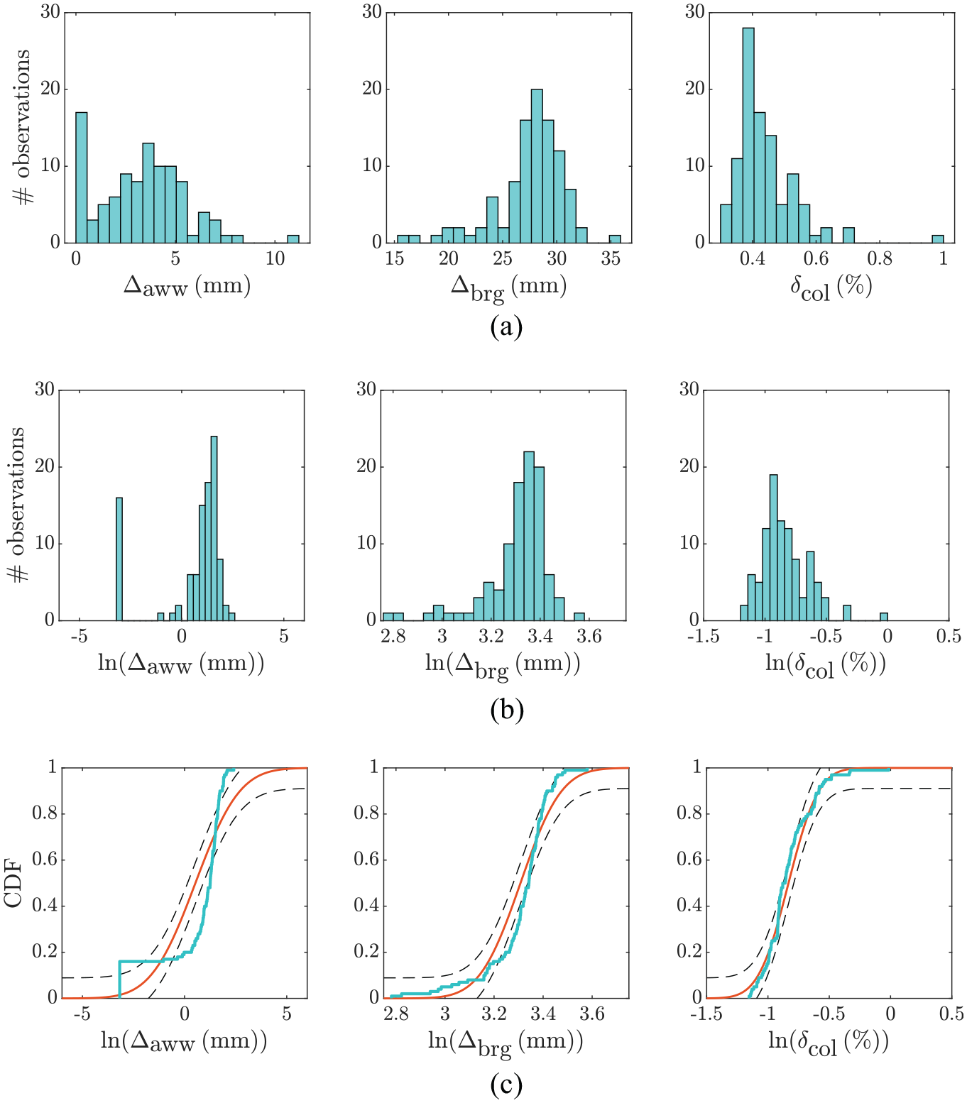
These different regimes, however, do not occur exclusively at specific levels of seismic intensity and Figure 5 is used to illustrate this phenomenon for spectral acceleration at $T_1$ of $0.8\mathrm{g}$ . For instance, if one focuses on the response of the elastomeric bearings, the bearing deforms freely with the deck on the verge of overcoming the gap in some cases, whereas, in other cases, the bearing has its deformation limited by the fact that the gap is closed and the wing walls resist the displacement of the ensemble deck/bearing pads. This is observed in Figure 5a by a first peak for ${\mathrm{\Delta }}_{\mathrm{brg}}<25.4\mathrm{mm}$ and a second greater peak for ${\mathrm{\Delta }}_{\mathrm{brg}}>25.4\mathrm{mm}$ . One can still notice these peaks after transforming the responses into the logarithmic space with the discontinuity separating the lower tail around $\ln (25.4)\approx 3.2$ (Figure 5b). Consequently, this lower tail with deformations that are less than $3.2$ causes the statistical test to fail (Figure 5c). In the case of deformation on abutment wing walls, one might infer that the fitted dispersion considering a lognormal distribution might be larger than the actual dispersion of the data due to the observation of null deformations (Figure 5b and c).

Figure 5.

Distribution of component demands for $S_a(T_1)=0.8\mathrm{g}$ : (a) histogram in original scale, (b) histogram in logarithmic scale, and (c) comparison of ECDF to test bounds (solid orange line represents the fitted lognormal CDF while dashed black lines indicate the bounds of the Lilliefors test).

It is therefore verified that, for the number of samples and the adopted significance level, the lognormal distribution may not satisfactorily represent the seismic responses of the components of a bridge at a set of $\mathrm{IM}$ levels of interest. A nonparametric approach, for instance, the kernel density estimator or logistic regression, could enhance the performance of the fitted marginal distribution of demand at each stripe (Karamlou and Bocchini, 2015; Mangalathu and Jeon, 2019). Nevertheless, a parametric approach such as the mixture of Gaussian distributions might also improve the modeling, as proposed in this study and verified later.

Assumptions on linear dependence

To assess the interaction between component responses, the Pearson correlation coefficient ${\rho }_{\mathrm{AB}}$ is usually employed (e.g. Ghosh et al., 2014; Nielson and DesRoches, 2007; Padgett and DesRoches, 2008), which is a measurement of the linear dependence between two random variables $A$ and $B$ and is bounded between $-1$ and $+1$ . This metric provides a very useful measure of dependence between variables: large values of $|{\rho }_{\mathrm{AB}}|$ imply strong stochastic dependence and a near-linear functional relationship, whereas small values may result from its lack of strong linearity if a functional relationship exists or from the predominance of other sources of variation (and hence low stochastic dependence) (Benjamin and Cornell, 1970). To the best of the authors’ knowledge, no study has been conducted on the validity of the assumption on linear dependence of seismic response between bridge components. However, the consequences on the definition of fragility of long bridges under nonuniform motion (i.e. with the effect of spatial variation of earthquake ground motions) were assessed by Lupoi et al. (2006), who also concluded that the correlation coefficients between piers were strongly dependent on the seismic intensity level and on the number of analyses, observing coefficients lower than unity even for adjacent piers under uniform motion.

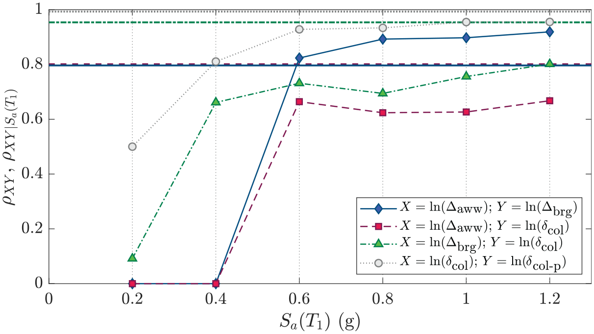
Despite these observations, some approaches still disregard the dependence of the correlation with respect to the $\mathrm{IM}$ level and compute the correlation coefficient using the whole demand dataset. This interpretation is believed by the authors to distort the real correlation between component demands, in the sense that demands tend to increase with the augmentation of the seismic intensity, and thus, the correlation coefficients would assume values close to unity. These values, however, are affected by the seismic intensity and do not represent the existing correlation between components. Accordingly, considering the entire demand dataset, the correlation coefficients independent of the IM level $({\rho }_{\mathrm{XY}})$ are estimated as follows: $0.797$ between abutment wing walls and elastomeric bearings; $0.800$ between abutment wing walls and bent columns; and $0.954$ between elastomeric bearings and bent columns. By leveraging the stripe structure of seismic demand using MSA, the correlation coefficients between component responses conditional on the seismic intensity are also estimated at each level of $S_a(T_1)$ $({\rho }_{\mathrm{XY}|S_a(T_1)})$ . These conditional values are presented in Figure 6 along with the independent values ${\rho }_{\mathrm{XY}}$ , in which the variation of the correlation coefficients with respect to intensity level is verified. One can also observe that the correlation coefficients involving the response on bent columns using the entire dataset are always higher than the conditional values.

Figure 6.

Evolution of correlation coefficients between component responses with respect to the seismic intensity.

The correlation between the drift of the two bents is also introduced into Figure 6 to assess the dependence between similar structural and spatially close components, although the drift of pinned columns $({\delta }_{\mathrm{col}-\mathrm{p}})$ are not taken as critical structural elements in the fragility analysis. The correlation coefficient between the columns of the two bents evolves from moderate $(\approx 0.5)$ to rather high correlation values (close to unity) with the increase of spectral acceleration, suggesting the dependence of the degree of correlation between pairs of bent columns to the level of seismic IM even for similar and adjacent structural components, as previously observed by Lupoi et al. (2006).

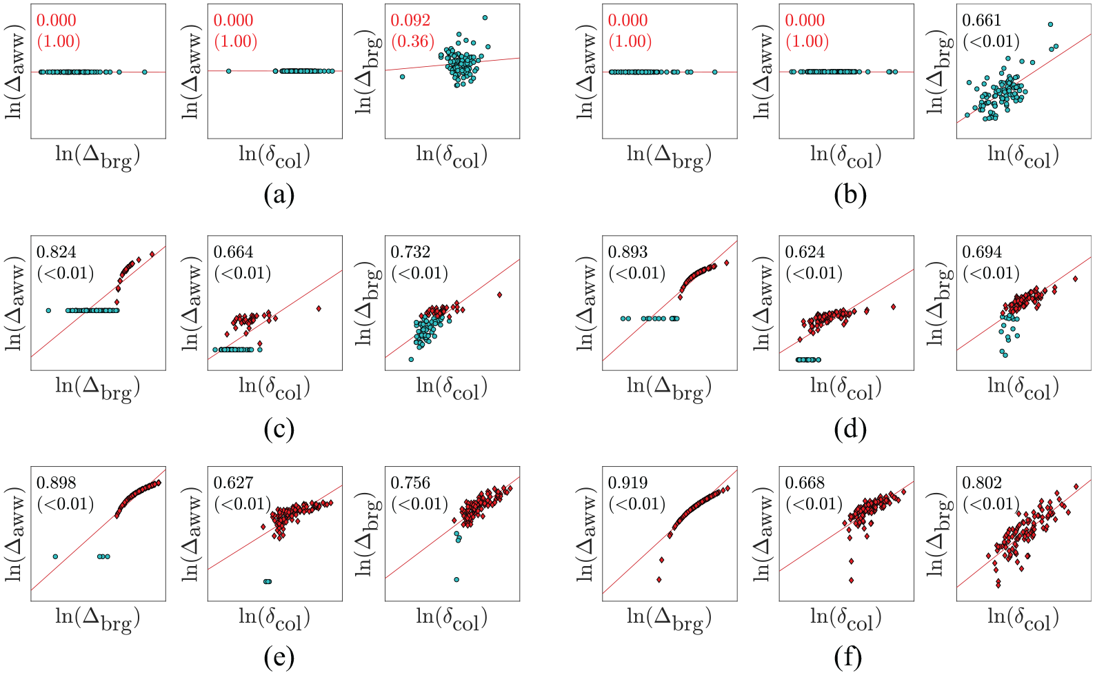
For low levels of seismic intensity (e.g. $S_a(T_1)=0.2\mathrm{g}$ ), the observed correlation coefficients are small ( $|{\rho }_{\mathrm{XY}|S_a(T_1)}|\le 0.1$ , except between column piers). As shown in Figure 6, the values of the correlation coefficient increase with the augmentation of the seismic intensity and values greater than $0.6$ are obtained for $S_a(T_1)\ge 0.6\mathrm{g}$ . This outcome might be seen as a tendency to linear dependence between the component demands from low to high $\mathrm{IM}$ levels, although for the in-between intensity levels, however, the relationship is not clear. Hence, it is of great importance to base this analysis on the visual inspection of the data as well as (and not only on) the computed correlation coefficients (Anscombe, 1973); Figure 7 illustrates the correlation plots at all the studied levels of spectral acceleration at the fundamental period.

Figure 7.

Correlation plots of pairwise component demands in the logarithmic space at each level of spectral acceleration (values on the upper corner indicate the correlation coefficients and the respective $p$ -values in between parentheses). Blue and red markers indicate open and closed gap, respectively: (a) $S_a(T_1)=0.2\mathrm{g}$ , (b) $S_a(T_1)=0.4\mathrm{g}$ , (c) $S_a(T_1)=0.6\mathrm{g}$ , (d) $S_a(T_1)=0.8\mathrm{g}$ , (e) $S_a(T_1)=1.0\mathrm{g}$ , and (f) $S_a(T_1)=1.2\mathrm{g}$ .

As observed, lower $S_a(T_1)$ levels (Figure 7a and b) show absent or low linear correlation with horizontally aligned (due to the gap between the abutment wing walls and the deck) or circular shaped graphed data. For responses at intermediate levels of spectral acceleration, for instance, $S_a(T_1)=0.6$ and $0.8\mathrm{g}$ (Figure 7c and d), graphed data indicate functional relationships that are clearly not linear, although correlation coefficients as high as $0.89$ may be observed. The closing of the gap may explain this behavior. As discussed in Figure 5, two deformation regimes are identified depending on the closure of the gap. Two colors are used on the markers in Figure 7 to distinguish the component demands with open (blue) or closed (red) gap, and the impact of this discontinuity on pairwise component correlation becomes evident. In these cases, a linear correlation coefficient may poorly model the dependence of the demand data. Finally, as previously stated, at higher levels of $S_a(T_1)$ , responses showed values of ${\rho }_{\mathrm{XY}|S_a(T_1)}$ close to unity, and the expected pattern of data for these values of the correlation coefficient are depicted in Figure 7e and f.

Furthermore, to test the absence of linear correlation between samples of two random variables $X$ and $Y$ (being the null hypothesis ${\rho }_{\mathrm{XY}}=0$ against the alternative hypothesis ${\rho }_{\mathrm{XY}}\ne 0$ ), considering that both come from a bivariate normal population, one can use the test statistic $T$ with Student’s $t$ -distribution for $n-2$ degrees of freedom to calculate the $p$ -value of the estimated correlation coefficient (Devore, 2004). It can also be used to establish the minimum sample size for a significant estimate of ${\rho }_{\mathrm{XY}}$ . For instance, more than $250$ samples are required to discard the absence of linear dependence between two random variables with correlation coefficients as low as $0.1$ at the $0.05$ significance level, whereas as few as $12$ samples are required for ${\rho }_{\mathrm{XY}}=0.5$ at the same significance level. The $p$ -values corresponding to the estimated correlation coefficients are also presented in parentheses in Figure 7.

Accordingly, for the lowest considered levels of $S_a(T_1)$ (e.g. Figure 7a), the observed $p$ -values of the correlation coefficients were greater than $0.05$ , which means that there is no strong evidence to show that these responses are linearly correlated. In the other cases (i.e. $S_a(T_1)>0.4\mathrm{g}$ ), the $p$ -values for the estimated correlation coefficients are always less than $0.05$ , indicating the rejection of the hypothesis that no correlation exists between the component responses. This rejection, however, does not ensure that the correlation is linear, as verified in Figure 7d, for example.

Hence, the linear correlation coefficient may not adequately capture the existing local dependencies between component seismic responses at some levels of seismic intensity, as observed at lower and intermediate levels of spectral acceleration in this case study. The proposed MSA-GM method considers correlation locally (e.g. within a mixture cluster) and might be more suitable for this task, as tested in the next section.

Fragility analysis based on MSA-GM

The proposed methodology based on coupling MSA and GM is first used to construct a GM seismic demand model for the observed data. Several models are fitted, and the capacity of the selected models to represent the observed data is assessed and compared to the unimodal case. The chosen model is then used to build component and system fragility curves for the case-study bridge. Finally, MSA-GM and other conventional strategies are used to assess the impact of some of the traditional hypotheses on fragility analysis.

Construction of the GM seismic demand model

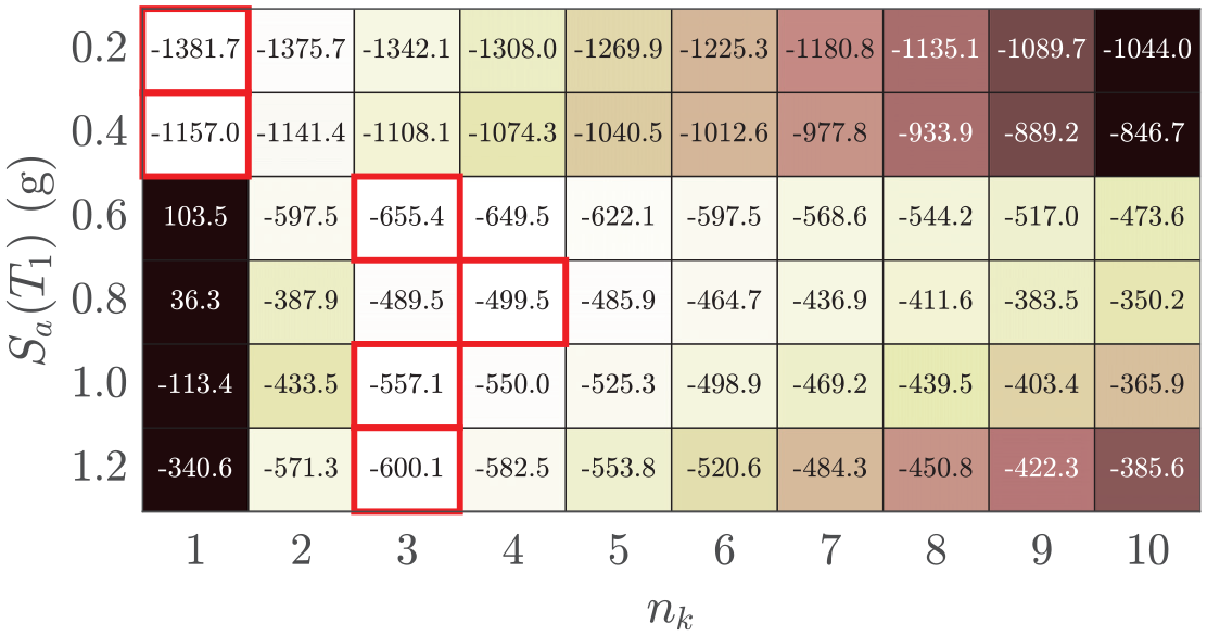
With the seismic demand data already presented and structured in stripes of spectral acceleration at $T_1$ , GM models are fitted for a number of mixture clusters ranging from $1$ to $10$ at each stripe. The maximum number of clusters is chosen to verify whether the chosen information criterion would be useful in selecting models that avoid overfitting. The covariance structure was defined as full-unshared, in which each cluster has its own covariance matrix with variance and correlation coefficients determined within the cluster. Although this option increases the number of hyperparameters per cluster, it tends to use fewer clusters to satisfactorily model the data than simpler covariance structures. The performance of each model is assessed using the BIC, and the values are shown in Figure 8. The selected number of mixture clusters is highlighted by red rectangles around the minimum values of BIC, and the color scale indicates the variation between the maximum (dark brown) and the minimum (white) BIC values at each stripe.

Figure 8.

BIC values for the Gaussian mixture models at each stripe (red rectangles indicate minima).

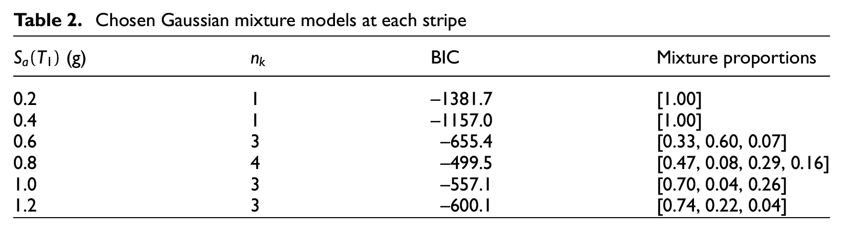
The final model is further detailed in Table 2, in which the proportion of each mixture cluster is also shown. In some cases, a small mixture proportion $(<0.1)$ is observed, indicating that small portions of the data are clustered, which might be seen as a sign of overfitting. Nevertheless, all selected models have four or fewer clusters, demonstrating that a reasonable trade-off between complexity and lack of fit is chosen. More stringent criteria could be adopted to choose simpler GM models and avoid selecting clusters with small proportions. For instance, it is observed in Figure 8 that GM models with only two mixture clusters perform almost as well as the selected clusters and could be chosen instead. Nevertheless, the chosen approach is to let the demand data speak for themselves.

Table 2.

Chosen Gaussian mixture models at each stripe

$S_a(T_1)$ (g)	$n_k$	$\mathrm{BIC}$	Mixture proportions
0.2	1	−1381.7	[1.00]
0.4	1	−1157.0	[1.00]
0.6	3	−655.4	[0.33, 0.60, 0.07]
0.8	4	−499.5	[0.47, 0.08, 0.29, 0.16]
1.0	3	−557.1	[0.70, 0.04, 0.26]
1.2	3	−600.1	[0.74, 0.22, 0.04]

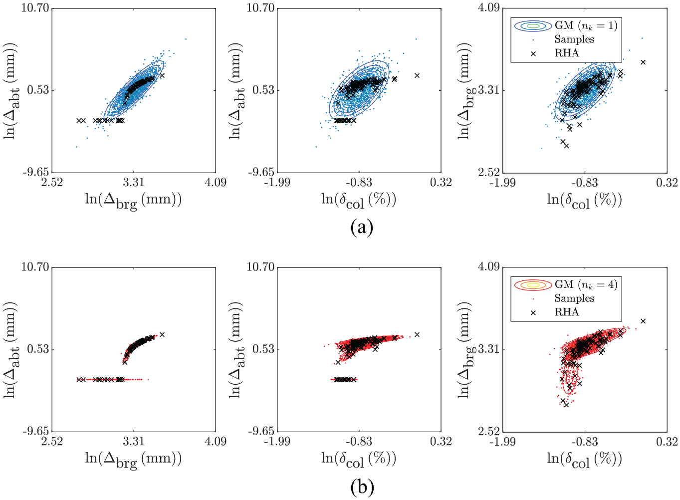
At low intensity levels ( $S_a(T_1)$ of $0.2$ or $0.4\mathrm{g}$ ), GM models with a single cluster may seem contradictory with respect to the statistical tests performed on the data (Figure 4). However, increasing the number of clusters to model the data at these levels of spectral acceleration does not show significant improvement to the density model as per the values of BIC (Figure 8). In the case of the abutment wing walls that are not mobilized at these levels of seismic intensity, as single-valued sample sets, they can be represented by a lognormal distribution with median equal to that value and a small dispersion (in the order of ${10}^{-2}$ ), with the marginal CDF approaching a step function without too much loss of information. In addition, it is important to notice the difference between the BIC of the chosen models and the one-cluster models for $S_a(T_1)$ in the range $0.6$ to $1.2\mathrm{g}$ ; these differences indicate the loss of information and the lack of fit when a unimodal multivariate lognormal distribution is fitted to the demand data at these stripes. This observation agrees with the values of the Lilliefors test statistic presented in Figure 4 that exceeds the critical value, especially for the deformation of abutment wing walls. An example to compare the sampling capabilities of the unimodal and the chosen model is graphically depicted in Figure 9 for $S_a(T_1)=0.8\mathrm{g}$ . One can recognize from the correlated samples that the unimodal approach generates a significant quantity of unrealistic demand samples (i.e. that do not agree with the observed data from RHAs), especially for the interactions with abutment wing walls. Although omitted for brevity, similar behavior is observed for spectral accelerations between $0.6$ and $1.2\mathrm{g}$ . Regarding the fragility analysis, these unrealistic drawn samples may introduce bias depending on the relevance of the components to the system fragility for a given damage state. To understand the relevance of each component to the system fragility, component and system fragility curves are determined from the final GM demand model and are presented next.

Figure 9.

Comparison of observed and sampled correlated demand data at $S_a(T_1)=0.8\mathrm{g}$ with: (a) one cluster and (b) four clusters.

Component and system fragilities

Fragility curves are assumed to follow a lognormal distribution with parameters $\mathbf{\Theta }=\{\theta ,\beta \}$ (i.e. median and dispersion). Hence, the CDF $F(\mathrm{im};\mathbf{\Theta })$ used in Equation 3 is:

$$F(\mathrm{im};\mathbf{\Theta })=\mathrm{Pr}(\mathrm{DS}|\mathrm{IM}=\mathrm{im})=\Phi \left(\frac{\ln (\mathrm{im}/\theta )}{\beta }\right)$$

(6)

where $\Phi (·)$ is the CDF of the standard normal distribution.

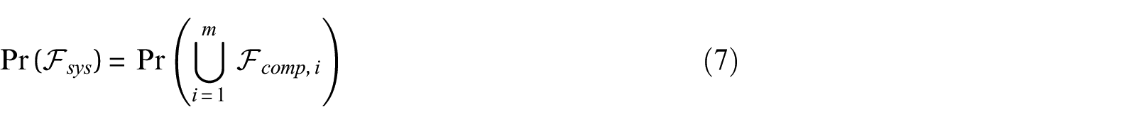
While many alternatives exist in the literature, a series system assumption is often adopted for the system damage state definitions of structures such as bridges (e.g. Nielson and DesRoches, 2007). Therefore, the violation of the same damage state of the system ${\mathcal{F}}_{\mathrm{sys}}$ is the union of the component violations, that is, ${\mathcal{F}}_{\mathrm{sys}}=\bigcup _{i=1}^m{\mathcal{F}}_{\mathrm{comp},i}$ , and thus, the probability of ${\mathcal{F}}_{\mathrm{sys}}$ is:

$$\mathrm{Pr}({\mathcal{F}}_{\mathrm{sys}})=\mathrm{Pr}\left(\bigcup _{i=1}^m{\mathcal{F}}_{\mathrm{comp},i}\right)$$

(7)

In addition, to conform the damage states of the components to the consequences to the bridge’s performance in terms of closure and repair implications, the components are classified as primary or secondary in accordance with their importance for bridge stability under traffic or a subsequent seismic event (Zakeri et al., 2014). Extensively damaged columns shall be classified as primary components, which are assumed to be the only components contributing to the probable replacement damage state of the bridge. Secondary components (e.g. abutments and bearings) are assumed to contribute to earlier damage states of the whole system (minimal, repairable, and extensive) because their complete failure will not have a similar consequence as that of primary components.

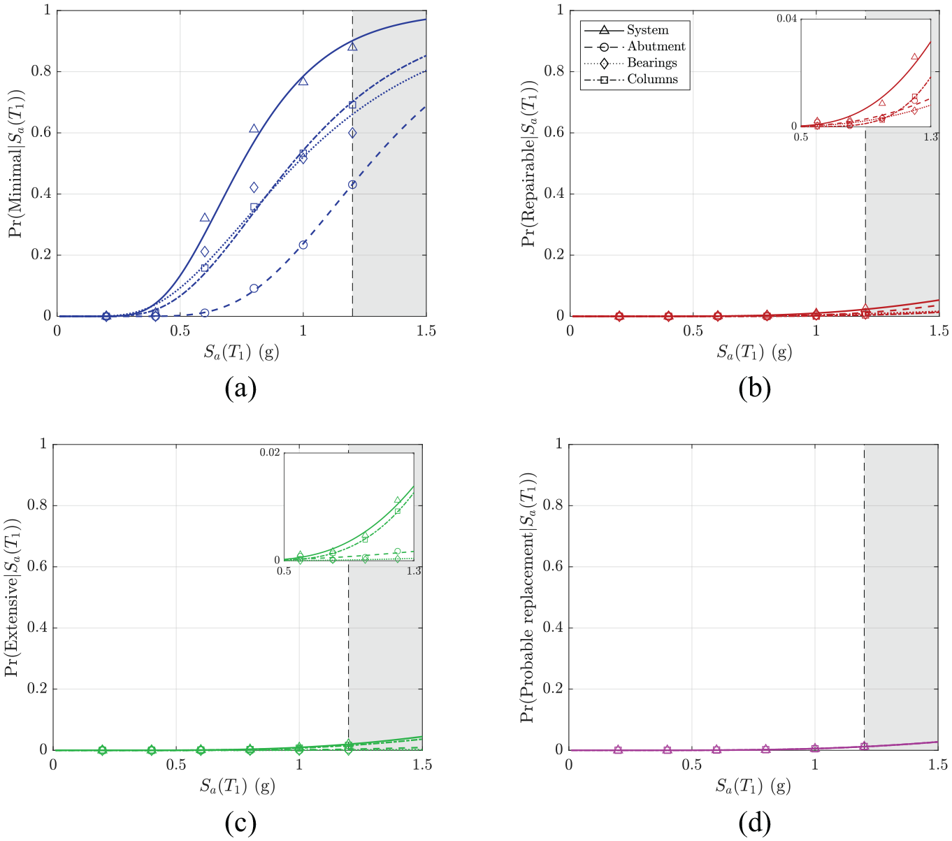
The fragility curves for the bridge components and for the whole system are fitted using the MLE, as in Equation 3. When MSA is performed, Baker (2015) recommends choosing $\mathrm{IM}$ levels near the lower tail of the fragility function and up to levels slightly above the median (i.e. with a fraction of observed damage state violation greater than $0.5$ ) to ensure a good fit. Figure 10 presents the fitted fragility curves for the four damage states for the system and critical components for spectral accelerations up to $1.5\mathrm{g}$ . Fragility curves for minimal damage follow the aforementioned strategy; conversely, the other fragility curves would show greater uncertainty, but the use of higher values of spectral acceleration would not be reasonable for the current case study.

Figure 10.

Fragility curves for components and system based on the MSA-GM model. Markers represent the fraction of observed violation of damage state and gray shaded areas indicate the region where the fragility curves extrapolate the investigated seismic intensity levels: (a) minimal, (b) repairable, (c) extensive, and (d) probable replacement.

The three critical components have a significant contribution to the system fragility for the minimal (Figure 10a) and repairable (Figure 10b) damage states (the latter being less likely with probabilities of less than $5\%$ ). Columns are the governing component for the extensive damage state, followed by the abutment wing walls that contribute to a lesser extent to the bridge fragility (Figure 10c). Only columns control the probable replacement of the bridge (as previously stated) (Figure 10d). Due to the performance criteria and column capacity adopted in the present work, abutment wing walls contribute more to the system’s repairable and extensive damage states than in a past study (Tavares et al., 2013). The system’s fragility is directly influenced by the fragility of each of the critical components for a given damage state, which in turn are intrinsically related to the capability of the PSDM strategy to model the observed demand data. This feature may be crucial when comparing the performance of PSDM strategies with different density modeling capabilities, as presented next.

Comparison of different hypotheses

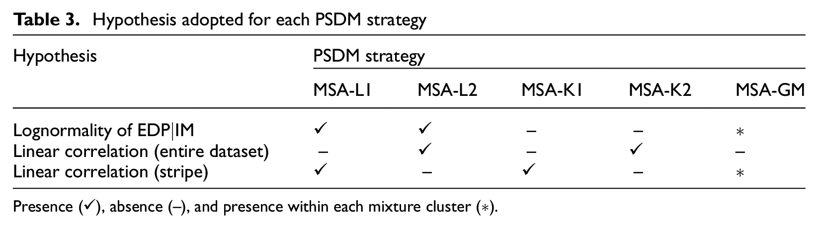
For this analysis, five different PSDM strategies are defined to isolate the effects of each of the investigated hypotheses, namely, MSA-L1, MSA-L2, MSA-K1, MSA-K2, and MSA-GM; Table 3 presents their characteristic assumptions. All strategies employ MSA for data collection, assuring heteroscedasticity of the demand with respect to the seismic intensity. In the adopted nomenclature, the letters indicate the statistical fitting of the demand data at each stripe: L stands for a multivariate lognormal distribution, whereas K stands for kernel density estimator (a nonparametric distribution as recommended by Karamlou and Bocchini, 2015). Finally, numbers 1 and 2 indicate, respectively, the assumption of correlation coefficient calculated at each stripe or using the complete dataset. Assuming that MSA-GM is the less constrained strategy, this demand model is taken as reference for comparing the impact of the adopted hypotheses to the results of the respective fragility analyses.

Table 3.

Hypothesis adopted for each PSDM strategy

Hypothesis	PSDM strategy
	MSA-L1	MSA-L2	MSA-K1	MSA-K2	MSA-GM
Lognormality of $\mathrm{EDP}|\mathrm{IM}$	✓	✓	–	–	*
Linear correlation (entire dataset)	–	✓	–	✓	–
Linear correlation (stripe)	✓	–	✓	–	*

Presence (✓), absence (–), and presence within each mixture cluster (*).

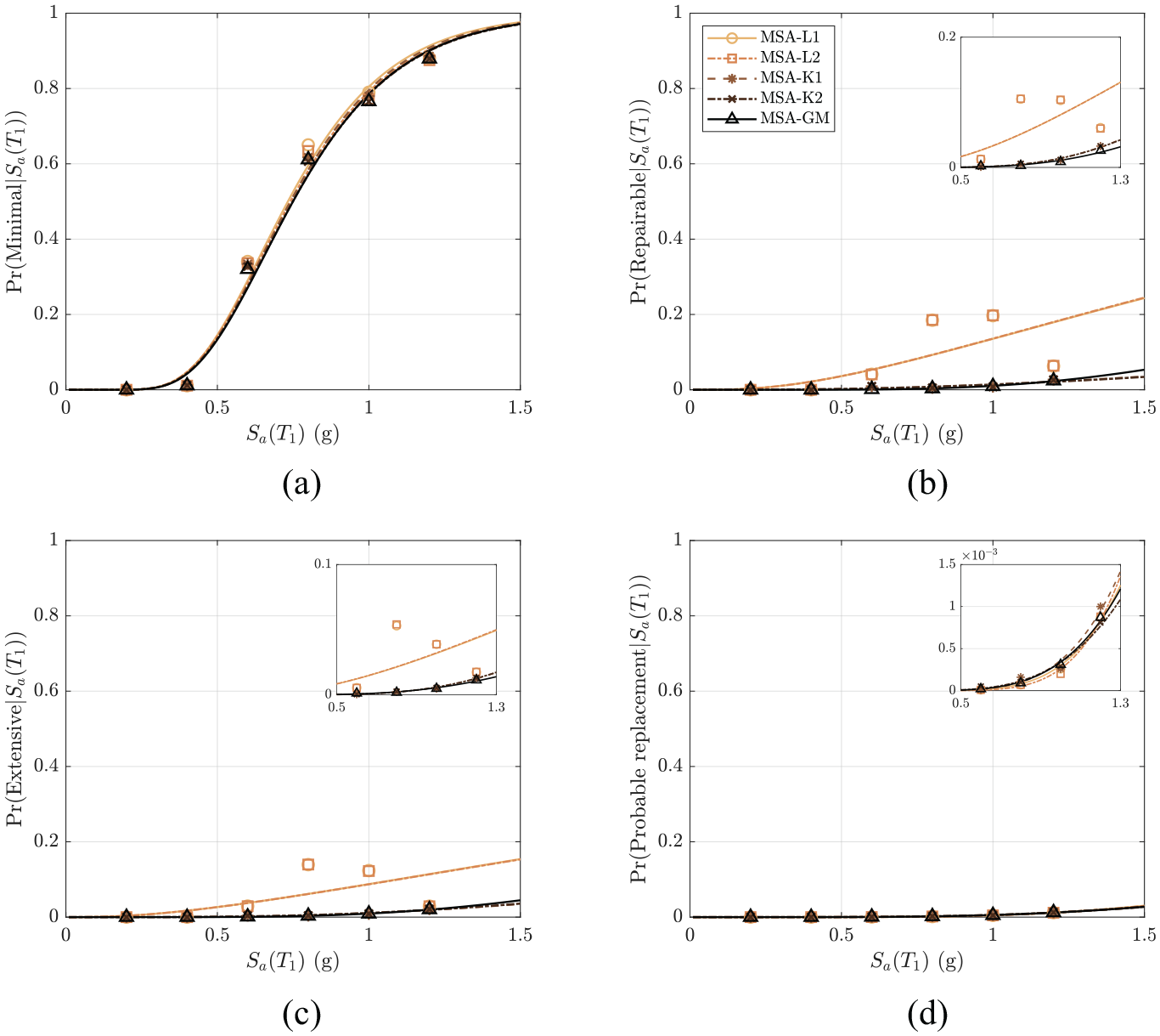
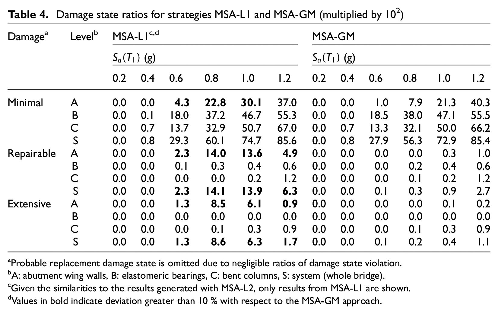
Figure 11 presents the system’s fragility curves obtained with each of the five PSDM strategies for all the damage states of interest. Strategies MSA-L1 and MSA-L2 performed similar to MSA-GM for minimal and probable replacement damage states, whereas the ratios of $\mathrm{DS}$ violation for repairable and extensive damage states are overestimated for intermediate stripes when compared to more flexible modeling strategies. As a consequence, the fitted fragility curves are drastically different from those obtained with the GM model and the kernel method. The overestimation is explained by the significant contribution of the abutment wing walls and columns to these system damage states and by the fact that these intermediate stripes represent $S_a$ at $T_1$ in the range from $0.6$ to $1.2\mathrm{g}$ , which are the same intensity levels at which the GM models were fitted with more than one mixture cluster (see Table 2). In addition, the ratios of $\mathrm{DS}$ violation produced by the lognormal strategies are not conventional, as they appear to oscillate for spectral accelerations between $0.6$ and $1.2\mathrm{g}$ with significant amplitude. This oscillation is attributed to the poor approximation of the lognormal distribution on the abutment wing wall deformation at these levels of spectral acceleration. A larger fitted dispersion than the actual dispersion (Figure 5) causes the model to draw unrealistic demand samples (Figure 9). As a consequence, the number of generated samples that exceed the component capacity tends to be higher than the actual fragility ratios (Table 4), indicating that the assumption of lognormality of the deformation of abutment wing walls introduced significant bias into the component and system fragility estimates, not being adequate for the investigated structure. Still from Table 4, it is worth noting that, despite violating the Lilliefors test at some intensity levels, the fragility estimates for elastomeric bearings and bent columns obtained with MSA-L1 are in good agreement with those generated with the MSA-GM approach. These results suggest that the unimodal lognormal distribution is a satisfactory approximation for the density modeling of bearing and column responses for the case-study bridge. These findings agree with the recommendations given by Karamlou and Bocchini (2015) that low bias may be introduced into fragility estimates if the maximum deviation between the ECDF and the hypothetical CDF of demand is less than $0.2$ .

Figure 11.

System fragility curves for different PSDM strategies with markers representing the fraction of observed violation of damage state: (a) minimal, (b) repairable, (c) extensive, and (d) probable replacement.

Table 4.

Damage state ratios for strategies MSA-L1 and MSA-GM (multiplied by 10²)

Damage a	Level b	MSA-L1c,d						MSA-GM
		$S_a(T_1)$ (g)						$S_a(T_1)$ (g)
		0.2	0.4	0.6	0.8	1.0	1.2	0.2	0.4	0.6	0.8	1.0	1.2
Minimal	A	0.0	0.0	4.3	22.8	30.1	37.0	0.0	0.0	1.0	7.9	21.3	40.3
	B	0.0	0.1	18.0	37.2	46.7	55.3	0.0	0.0	18.5	38.0	47.1	55.5
	C	0.0	0.7	13.7	32.9	50.7	67.0	0.0	0.7	13.3	32.1	50.0	66.2
	S	0.0	0.8	29.3	60.1	74.7	85.6	0.0	0.8	27.9	56.3	72.9	85.4
Repairable	A	0.0	0.0	2.3	14.0	13.6	4.9	0.0	0.0	0.0	0.0	0.3	1.0
	B	0.0	0.0	0.1	0.3	0.4	0.6	0.0	0.0	0.0	0.2	0.4	0.6
	C	0.0	0.0	0.0	0.0	0.2	1.2	0.0	0.0	0.0	0.1	0.2	1.2
	S	0.0	0.0	2.3	14.1	13.9	6.3	0.0	0.0	0.1	0.3	0.9	2.7
Extensive	A	0.0	0.0	1.3	8.5	6.1	0.9	0.0	0.0	0.0	0.0	0.1	0.2
	B	0.0	0.0	0.0	0.0	0.0	0.0	0.0	0.0	0.0	0.0	0.0	0.0
	C	0.0	0.0	0.0	0.1	0.3	0.9	0.0	0.0	0.0	0.1	0.3	0.9
	S	0.0	0.0	1.3	8.6	6.3	1.7	0.0	0.0	0.1	0.2	0.4	1.1

a

Probable replacement damage state is omitted due to negligible ratios of damage state violation.

b

A: abutment wing walls, B: elastomeric bearings, C: bent columns, S: system (whole bridge).

c

Given the similarities to the results generated with MSA-L2, only results from MSA-L1 are shown.

d

Values in bold indicate deviation greater than 10 % with respect to the MSA-GM approach.

Fragility curves based on strategies MSA-L1 and MSA-L2 are practically superposed. This is also observed in fragility curves for MSA-K1 and MSA-K2. Therefore, one can conclude that the impact of the correlation using the entire dataset compared to the stripewise approach was negligible on the resulting fragilities for the case-study bridge, and Figure 6 may explain this finding. Correlation coefficients independent of the level of $S_a(T_1)$ were particularly different from the dependent values for spectral accelerations below $0.4\mathrm{g}$ , and no damage state violation was observed at these stripes. In addition, the good agreement between the fragility curves fitted with samples from the nonparametric strategies (MSA-K1 and MSA-K2) and the parametric model MSA-GM allows one to conclude that (1) the latter was able to fit a parametric density model that was equivalent to the nonparametric distribution fitted by kernel smoothing and that (2) the consideration of linear correlation between components did not significantly affect the fragility in the present case study. This second statement contradicts the observations made by Lupoi et al. (2006) for long bridges under nonuniform ground motions. The differences in the investigated structures may explain the divergent conclusions with respect to the impact of the correlation between components.

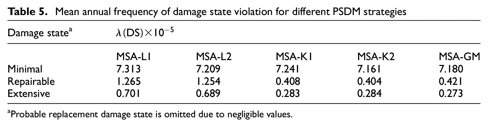
Finally, the MAF of violating a damage state is intrinsically related to the fragility. Table 5 presents the MAF of damage state $\lambda (\mathrm{DS})$ calculated with each PSDM strategy investigated for all the considered damage states. As expected, intermediate damage states (repairable and extensive) show the greatest differences due to previously observed nonconform fragility curves. Accordingly, differences of more than $100\%$ are observed when lognormality was incorporated, indicating the bias introduced by poor statistical modeling. This difference could be crucial in accepting the performance of a structure if a threshold for the probability of failure is to be respected. For instance, the MAFs of repairable damage state calculated using MSA-L1 and MSA-GM represent a difference in terms of probability of exceedance in $50$ years of $0.4\%$ . In the case of extensive damage state, however, the difference may be found to be negligible given that it represents extremely rare events with return periods greater than 100,000 years. Despite its outdated seismic detailing, the bridge presents overall satisfactory performance, which may be attributed to its location on a region of low to moderate seismicity.

Table 5.

Mean annual frequency of damage state violation for different PSDM strategies

Damage state a	$\lambda (\mathrm{DS})\times {10}^{-5}$
	MSA-L1	MSA-L2	MSA-K1	MSA-K2	MSA-GM
Minimal	7.313	7.209	7.241	7.161	7.180
Repairable	1.265	1.254	0.408	0.404	0.421
Extensive	0.701	0.689	0.283	0.284	0.273

a

Probable replacement damage state is omitted due to negligible values.

Conclusion

A methodology coupling MSA and GM models is proposed for the construction of multivariate seismic demand models with the objective of improving fragility analysis of specific multicomponent structural systems, such as highway bridges. This methodology exploits the stripe structure provided by MSA to locally assess the statistics of the relationship $\mathrm{EDP}|\mathrm{IM}$ ; and the flexibility of mixture models to find density functions that better fit the data given the cluster structure. This approach is thus less constrained than traditional seismic demand modeling strategies in the sense that it does not rely on the typical hypotheses, namely, unimodal lognormality, homoscedasticity, and linear dependence between components.

A classic multispan continuous concrete girder bridge in Eastern Canada is used as a case study to demonstrate the application of the proposed method and to investigate its performance. Initially, a rigorous ground motion selection is performed to define a statistically significant suite of records to then produce the seismic demand data following the scheme of MSA. The proposed approach showed enhanced capacity in fitting the data when compared to traditional approaches that employ lognormal distribution (which is similar to the single-cluster models). A density function that satisfactorily fits the observed data avoids the introduction of bias into the fragility analysis. This effect is also verified when the features of the proposed MSA-GM model are leveraged for the construction of system fragility functions and calculation of the MAF of damage state violation.

In addition to the fragility analysis, the produced demand data are investigated with respect to the validity of lognormality and linear dependence. First, the Lilliefors test—a more suitable test for goodness of fit of normal distributions—is employed in the verification of lognormality, and confirming a general perception, this hypothesis is not valid at several $\mathrm{IM}$ levels for all the components (especially in the case of abutment wing walls with a gap). The impacts of this assumption on the system fragility analysis are significant for intermediate damage states, indicating that the governing structural components must be appropriately modeled when assessing the system fragility. The hypothesis on the linear dependence between components is also investigated using graphic inspection and testing the absence of correlation, concluding that this assumption is not always valid either. It is shown that the correlation coefficient varies gradually with the augmentation of the spectral acceleration. This observation does not agree with the commonly adopted approach of a constant correlation coefficient over all $\mathrm{IM}$ levels. These assumptions, however, have negligible impact on the fragility analysis of the case-study bridge. The analysis of a conventional bridge under uniform motion may explain this finding.

Due to irregularities, asymmetries, and discontinuities, structural systems with highly complex component interactions or multiple regimes of behavior may indeed violate traditional assumptions. Accordingly, the gap between the deck and the abutment wing walls in the case-study bridge causes a discontinuity in the response not only on the deformation of wing walls but on the other critical components by impacting their statistical distribution and dependence. This discontinuity is identified as a driver that leads to the demand data failing the statistical test on lognormality and to the lack of linearity between components. Two regimes of deformation of the bridge components are distinguished relative to gap closure, which depend on the earthquake intensity although not exclusive to a certain intensity level. The proposed density modeling strategy can identify these two regimes and build a more refined multivariate PSDM. The hypotheses of lognormality and linear correlation may, however, still be valid or represent suitable approximations of the observed data depending on the specific structure and on the level of acceptable error on the risk assessment. The choice on the strategy to perform probabilistic seismic demand modeling that better suites the investigated data remains the analyst’s responsibility.

The application of the model is demonstrated using a typical highway bridge with satisfactory seismic performance even though the structure was conceived without stringent seismic design rules at the time. Structures with insufficient seismic detailing in higher seismicity regions and long bridges may be prime candidates to confirm the advantages of the proposed approach. Poor seismic detailing may be the driver of complex component interactions and multiple regimes of nonlinear behavior, while the effect of multiple support motions in long bridges may require refined component dependence modeling. Structural modeling parameters that are neglected in the present study should be incorporated in future work. For instance, strain penetration at the intersection of columns and footings and bridge joints affects the response of bents, which may impact the complexity of the structural demand. Likewise, as design codes are improved periodically, new performance criteria and corresponding component damage indicators should be updated in future bridge fragility assessments. The application of the proposed approach to the construction of bridge-specific fragility functions should also be expanded and tested for the assessment of bridge classes and regional portfolios. Finally, the model could be employed for a thorough analysis of other multicomponent structures, such as multistory buildings in which the responses of different elements or distinct EDPs might be correlated.