Sage Journals: Discover world-class research

Abstract

This article develops seismic capacity models for earth dams and demonstrates how the proposed seismic capacity models may be used to develop seismic fragility curves that predict the probability of damage as a function of ground shaking intensity. Developing earth dam fragility curves requires two major components: (1) a seismic capacity model that predicts the probability of a damage state given the relative settlement (RS) and (2) an engineering demand model that predicts the RS as a function of ground motion intensity. While seismic demand models for earth dams have been studied by various researchers, there is a scarcity of seismic capacity models. This article focuses first on developing seismic capacity relationships using a dataset of earthquake case histories of dam performance. Different from previously developed relationships, only the damage description for each dam is used when assigning the damage state, which results in statistical variability in the capacity relationship between the damage state and RS. The fragility curve development is demonstrated by combining the seismic capacity relationships with a seismic demand model for RS derived from nonlinear, dynamic finite element analyses for a 20-m generic dam geometry subjected to a suite of earthquake motions from the NGA-West2 database.

Keywords

Seismic fragility model seismic capacity relationships earth dams

Introduction

According to the National Inventory of Dams database, there are more than 91,000 dams across the United States and they have an average age of 57 years. Earthquake shaking can cause considerable damage to earth dams (Ambraseys, 1960; Harder et al., 1998; Seed et al., 1978), and thus it is important for dam owners to evaluate the seismic performance of these dams. However, performing individual site-specific analysis for a large portfolio of dams is unrealistic. Fragility models, which predict the probability of different damage states for a given ground shaking intensity measure (IM), can be used to assess the potential seismic risks to a portfolio of dams given the regional seismic hazard or they can be used to quickly evaluate the potential of damage to dams after an earthquake (Fraser et al., 2008).

Fragility models can also be utilized in the performance-based earthquake engineering (PBEE) framework (Moehle and Deierlein, 2004) to assist stakeholders to make informed decisions based on predicted economic losses and fatalities. The PBEE framework consists of four main components, seismic hazard analysis to define the ground shaking IM, engineering analysis to compute the engineering demand parameter (EDP), damage analysis to evaluate the damage measure (DM), and loss assessment to predict the decision variable (DV). The IM is represented by a ground motion hazard curve given regional seismic hazard. Numerical engineering analysis is performed to calculate the EDP given ground motions that are consistent with the regional seismic hazard. Damage analysis translates the EDP to a DM, which describes the physical damage of the structure. Finally, the DV is calculated, which represents a parameter or parameters that are meaningful to decision makers, such as losses or downtime. The annual rate of the DV being exceeded, ( $v (DV)$ ), can be expressed in terms of IM, EDP, and DM through a triple integral based on the total probability theorem:

v (DV) = \int \int \int G 〈 DV | DM 〉 | dG 〈 DM | EDP 〉 | dG 〈 EDP | IM 〉 | d λ (IM),

(1)

where $d λ$ is the annual rate of occurrence for each IM level, $G$ is a complementary cumulative density function (CCDF), and $dG$ is a derivative of the CCDF.

The full triple integral does not need to be employed to utilize PBEE to gain insight into the seismic performance of a system. Kramer (2008) discusses the different levels of implementation of PBEE: response level (which focuses on the EDP), damage level (which focuses on the DM), and loss level (which focuses on the DV). For example, geotechnical engineers have developed hazard curves for EDP such as slope displacement (e.g. Rathje and Saygili, 2008) or lateral spreading (Franke and Kramer, 2014) by using only the first two components of Equation 1. However, geotechnical engineers less often implement damage-level or loss-level PBEE. Recent studies regarding earth dam fragilities (Pang et al., 2019; Regina et al., 2023; Yang, 2021) have focused on response-level implementations of PBEE using Equation 1. In these previous studies, the EDP is often computed by performing a series of numerical analyses using a suite of input ground motions at different IM levels, but the DM or damage state is assigned deterministically based on threshold levels of EDP.

To improve the state of art in seismic dam fragilities, this study builds off of a fragility framework that was discussed in Rathje and He’s (2022) study. This framework consists of two major components: (1) a probabilistic seismic demand model that predicts the value of the EDP for a given ground motion IM and (2) a probabilistic seismic capacity model that relates the relevant damage state with a given EDP. These two models are used together to compute the resulting fragility model. Such fragility framework not only considers the uncertainties involved in the demand model, but also captures the variabilities in the capacity model, which allows one to access earth dam performance probabilistically within the damage-level implementation.

Because the development of seismic demand models has been studied more extensively in the literature, this study focuses first on the development of seismic capacity models for earth dams. The relative settlement (RS) of the dam crest, which has been found to be a good indicator of damage to earth dams (Fell et al., 2000; Swaisgood, 1998), is used as the EDP. Although cracking may be another indicator of earth dam damage, it is not easily or directly predicted through engineering analysis and is not considered as an EDP in this research. A dataset of earthquake case histories of dam performance is compiled and used to develop seismic capacity relationships, which relate the RS to each damage state. Here, observed damage is used to assign the damage state to each dam case history. The developed seismic capacity relationships are then used in a hypothetical example that demonstrates the use of the framework to derive a seismic fragility relationship for a 20-m earth dam. The demand model used in the example is derived from RSs computed from nonlinear finite element analyses subjected to earthquake time histories recorded for a range of intensities from the NGA-West2 (Ancheta et al., 2014) database.

Seismic fragility framework

Seismic fragility curves predict the probability of a damage state given the IM of an earthquake ground motion. The approach used in this article to develop the seismic fragility curves is also commonly utilized in structural earthquake engineering (e.g. Celik and Ellingwood, 2010; Kennedy and Ravindra, 1984; Khosravikia et al., 2020; Nielson and DesRoches, 2007; Ramanathan, 2012). The probability of a structure meeting or exceeding a predefined damage state (e.g. minor, major, collapse) can be computed using a conditional probability. It is computed as the probability of the demand, D, meeting or exceeding the capacity for that damage state, $C_{DS}$ , given the ground IM (e.g. peak ground acceleration (PGA); peak ground velocity (PGV)):

P_{DS} = P [D \geq C_{DS} | IM]

(2)

Within the PBEE framework, the demand model serves as the outcome of the response-level analysis, which computes the expected EDP given the IM; while the capacity model is the outcome of damage-level analysis, which predicts the level of damage state (or DM) given the EDP.

Figure 1 presents a schematic of the process used to develop seismic fragility curves for earth dams. The seismic demand model is developed from nonlinear response analysis, where representative numerical models of earth dams are subjected to a suite of ground motions. The EDP is computed for each analysis, plotted against the corresponding IM of the input motion, and an expression is developed to predict the EDP as a function of the IM. Earthquake case histories are used to develop the seismic capacity models. These case histories require that both the observed damage state of a dam and the measured EDP are available. The seismic demand and capacity models, along with their variabilities, are used together to obtain the final fragility curves either through Monte Carlo simulations or closed-form solutions.

Figure 1.

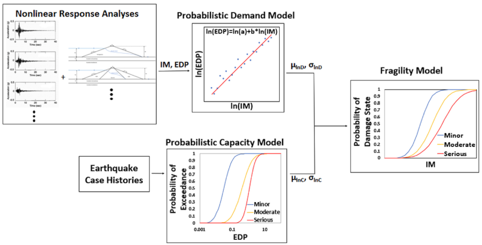
Flowchart describing the components used to develop seismic fragility curves (after Khosravikia et al., 2020).

Probabilistic seismic demand model

The seismic demand model predicts the median of the EDP as a function of the ground motion intensity. For the development of the demand model, the numerical model is subjected to a suite of N ground motions, and the peak value of the EDP for each motion is recorded as the demand ( $D$ ). The demand parameter often is assumed to follow a power law function in terms of the IM (Cornell et al., 2002), which can be expressed as:

D (IM) = a \cdot I M^{b}

(3)

By taking the natural logarithm of both sides of the equation, the relationship may be transformed into its linear form:

\ln (D) = μ_{\ln D} = \ln (a) + b \cdot \ln (IM),

(4)

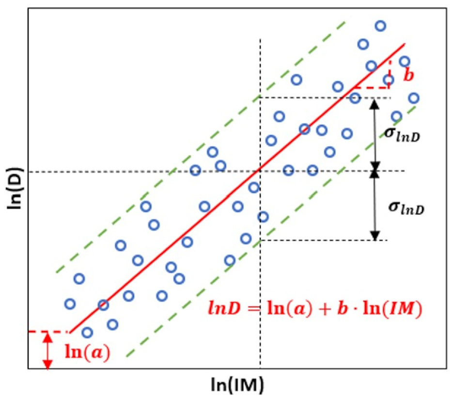
where the model parameter $\ln (a)$ is the vertical intercept and the parameter b is the slope of the relationship in terms of $\ln (IM)$ and $\ln (D)$ , as shown in Figure 2. More complex functional forms may be used for the demand model, if necessary.

Figure 2.

Linear regression of the engineering demand model (after Ramanathan, 2012).

This functional form assumes that the EDP follows a lognormal distribution, with the mean of the natural log ( $μ_{\ln D}$ ) given by Equation 4 and the standard deviation ( $σ_{\ln D}$ ) computed by:

σ_{\ln D} = \sqrt{\frac{\sum_{i = 1}^{N} {[\ln (D_{i}) - μ_{\ln D, i}]}^{2}}{N - 2}},

(5)

where $D_{i}$ is the recorded maximum value of the EDP for input motion i, $μ_{\ln D, i}$ is the natural log of the EDP predicted from Equation 4 for the IM of motion i, and N is the number of input motions.

Probabilistic seismic capacity model

The seismic capacity model defines the damage state as a function of the selected EDP and can be developed by relating damage states to the observed EDP. Field observations or laboratory experiments, in which both the damage state and the observed EDP are recorded, may be used to develop capacity models. If the capacity level of the EDP (i.e. $C$ ) is exceeded, the structure has exceeded the damage state and is expected to experience the corresponding damage state or larger. To account for variability in the EDP capacity, it is assumed that the capacity for each damage state follows a lognormal distribution with a mean of $μ_{\ln C}$ and associated standard deviation of $σ_{\ln C}$ .

As an example, consider the development of a seismic capacity model for masonry walls described by Khosravikia et al. (2020). The EDP used for the masonry wall was the veneer tie deformation because it was directly correlated to the out-of-plane brick veneer damage. Based on their literature review and preliminary numerical analyses, it was found that brick ties were assumed to fail at deformations larger than 6.85 mm. To account for uncertainty in the deformation capacity of the ties, Khosravikia et al. (2020) assumed that the capacity for the damage state followed a lognormal distribution with $μ_{\ln C}$ , given as the previously stated deformation capacity, and dispersion of $σ_{\ln C}$ . The coefficient of variation (COV) was assumed to be 25% and the resulting $σ_{\ln C}$ computed to be 0.247 using the following.

σ_{\ln C} = \sqrt{\ln (1 + CO V^{2})}

(6)

The development of such a seismic capacity model for earth dams is a critical aspect of this article and will be discussed in greater detail subsequently.

Probabilistic fragility relationship

Given the engineering demand and seismic capacity models along with a ground motion intensity level (IM), a fragility relationship can be derived for each damage state. The fragility relationship can be derived from a closed-form solution if the demand and capacity models are lognormally distributed and only one EDP is considered. In this case, Equation 2 can be written directly in terms of the statistical parameters of the demand and capacity models:

P_{DS} = P [D \geq C_{DS} | IM] = Φ [\frac{\ln (IM) - μ_{DS}}{β_{DS}}],

(7)

where $Φ [\cdot]$ is the standard normal cumulative distribution function. When only one demand parameter and one IM are used, the mean and standard deviation of a lognormal fragility curve for a specific damage state (i.e. $μ_{DS}$ , $β_{DS}$ ) can be directly computed using the coefficients of the demand and capacity models. Based on the work of Cornell et al. (2002) and Yang (2021), $μ_{DS}$ and $β_{DS}$ of the fragility curves can be computed as:

μ_{DS} = \frac{μ_{\ln C} - \ln (a)}{b}

(8)

β_{DS} = \frac{\sqrt{{σ_{\ln D}}^{2} + {σ_{\ln C}}^{2}}}{b}

(9)

In situations where the demand and/or capacity models are not lognormally distributed or the system fragility is characterized by multiple EDPs, a Monte Carlo simulation can be used to obtain the fragility curves (e.g. Khosravikia et al., 2020; Padgett and DesRoches, 2008; Ramanathan 2012). For each Monte Carlo sample j, independent values of the error term ε for the capacity ( $ε_{C, j}$ ) and for the demand ( $ε_{D, j}$ ) are statistically generated from a normal distribution with mean of 0 and standard deviation of 1 and used to compute the capacity and demand as:

C_{j} = \exp (μ_{\ln C} + ε_{C, j} \cdot σ_{\ln C})

(10)

D_{j} = \exp (μ_{\ln D} (IM) + ε_{D, j} \cdot σ_{\ln D})

(11)

For each Monte Carlo sample, it is defined that a damage state is exceeded if demand is larger than or equal to the capacity (i.e. $D_{j} \geq C_{j}$ ). The probability of damage for each IM value is calculated as the percentage of Monte Carlo samples in which $D_{j} \geq C_{j}$ after running a large number (i.e. 10⁶) of Monte Carlo samples. This computation is carried out for a range of IM values to create the fragility curve for each damage state.

Previous studies on seismic dam fragilities

Some recent studies have developed seismic fragility curves for earth dams. Regina et al. (2023) performed seismic performance analysis of two earth dams in Southern Italy. Relationships between different IMs and different EDPs (i.e. filter displacement, global instability, free board reduction, excess pore water pressure ratio) were developed, as well as fragility relationships using the Pells and Fell (2002) damage states. Pang et al. (2019) and Yang (2021) provided fragility relationships that relate IMs to different damage states, but the capacity models used for both studies do not consider variabilities in the capacity of the earth dams. For example, Yang (2021) defines damage state 1 as having crest settlement larger than 10 cm. Thus, only variabilities in the demand model contribute to the final fragility model.

To account for variabilities in both the capacity and demand models for earth dams, this article aims to develop seismic capacity models that consider statistical variability in the relationship between EDP and damage state, and then the proposed capacity models are used within Monte Carlo framework to develop fragility curves for a hypothetical 20-m homogeneous dam.

Development of seismic capacity model for earth dams

Damage assessment of earth dams

Seismic capacity models for earth dams can be developed based on observations of dam performance from earthquake case histories. The different types of damage that may result from earthquakes include cracking, sliding, post-earthquake internal erosion, and so on (Pells and Fell, 2002). While a dam may experience one or more of these types of damage, deformation is a good indicator of damage and it can be computed and visualized from engineering analyses. Deformation can be manifested as vertical or horizontal movement of the dam crest or along the dam slopes, and various studies have shown that the damage level of an earth dam is closely related to the $RS$ of the dam crest (Fell et al., 2000; Swaisgood, 1998). $RS$ is calculated as the ratio of the settlement of the dam crest to the dam height:

RS (%) = \frac{Crest settlement}{Dam height} \times 100

(12)

where the dam crest settlement is the displacement of the dam crest in the vertical direction, and the dam height is the original dam height before any deformation (Figure 3). RS as the EDP accounts for the vertical effects of deviatoric sliding deformation, co-seismic volumetric deformation, as well as possible post-liquefaction volumetric recompression, and it is assumed that RS indicates the potential for cracking of the dam. Swaisgood (2003) recommended defining the EDP as the settlement normalized by the combined dam height and thickness of the alluvium foundation soils, but foundation alluvium thickness was not available for many of the case histories considered and may not be available for all dams being evaluated with the fragility models. In addition, although the characteristics of the foundation soils certainly impact the crest settlement of a dam, Pells and Fell (2002) questioned whether it is warranted to include the alluvium thickness in the normalization of the crest settlement. Thus, we chose not to include it in the EDP definition.

Figure 3.

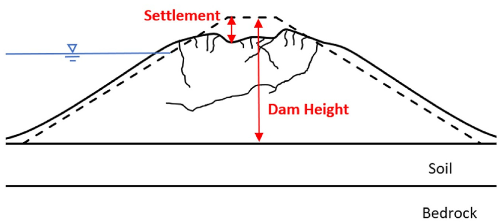
Idealized drawing of deformed earth dam (after Ambraseys, 1958, taken from Yan, 1991).

Previous capacity models

Previous studies have developed seismic capacity relationships for earth dams based on field observations of performance (Pells and Fell, 2002; Swaisgood, 2003). However, in these studies the damage state was assigned to each dam considering both the observed cracking (i.e. damage) and the observed RS (i.e. EDP), which makes the relationship between EDP and damage state somewhat circular. For example, the Pells and Fell (2002) capacity relationships (Table 1) include six different damage states ranging from no/slight damage to collapse, and each damage state is associated with a corresponding range of maximum longitudinal crack width and maximum relative crest settlement. Because the damage state is directly related to non-overlapping thresholds of the demand parameters (i.e. relative crest settlement), the capacity relationships effectively are step functions without any variability, as shown in Figure 4. The seismic capacity relationships developed by Swaisgood (2003) used a similar approach with RS as the only EDP, although with different damage states and thresholds.

Table 1.

Capacity relationships for earth dams proposed by Pells and Fell (2002)

Damage class		Maximum longitudinal crack width (cm)	Maximum relative crest settlement (%)
Number	Description	Maximum longitudinal crack width (cm)	Maximum relative crest settlement (%)
0	No or slight	<1	<0.03
1	Minor	1–3	0.03–0.2
2	Moderate	3–8	0.2–0.5
3	Major	8–15	0.5–1.5
4	Severe	15–50	1.5–5
5	Collapse	>50	>5

Figure 4.

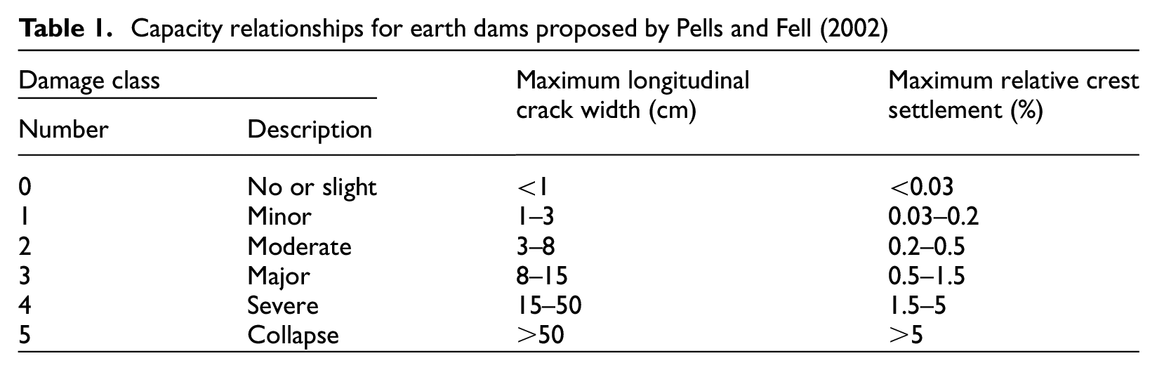
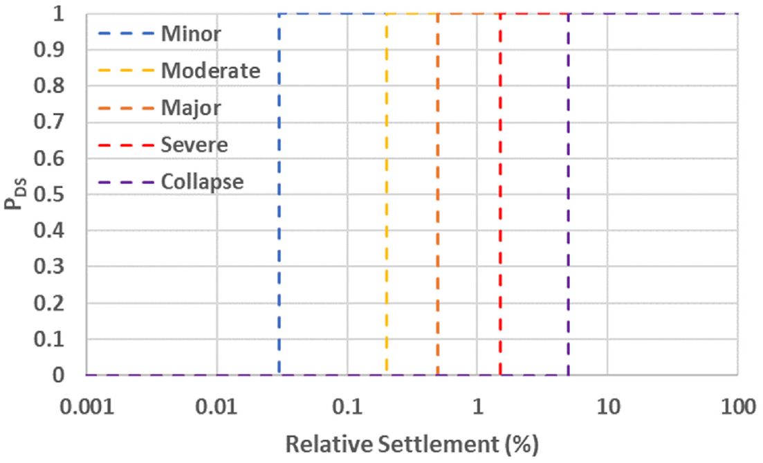
Seismic capacity relationships for earth dams from Pells and Fell (2002).

To address this circularity issue and to incorporate statistical variability in the capacity relationships, the damage state assessments used in this study are based on the field damage observations (including crack width and patterns) as reported by the original authors, regardless of the RS. Then the statistics of the RS for the case histories associated with each damage state are analyzed to develop the capacity relationships. A database comprising earthquake case histories from multiple sources is first developed and then used to define the capacity relationship for each damage state. This work updates previously developed capacity relationships from Rathje and He (2022).

Development of database for observed earth dam performance

Previous studies have collected case histories of earth dam performance during earthquakes. Two major studies initially are considered: Pells and Fell (2002) and Swaisgood (2003). Pells and Fell’s (2002) study includes a database of over 300 dam incidents that was compiled to study the settlement, deformation, and cracking of embankment dams during earthquakes. Swaisgood’s (2003) study reviewed nearly 70 case histories of embankment dam deformations caused by earthquakes to determine the relationship between damage state and seismic deformation of earth dams. However, not all the 370 case histories from these two sources can be used in this study because only a small portion of the case histories provides values of RS, and there are overlapping case histories between the two databases. After reviewing both studies, 77 case histories were selected, each of which contains a quantitative record of RS and a field assessment of the damage state/cracking. To include case histories from more recent earthquake events and to better populate some of the damage states, another 17 case histories were added to the database from other sources, which include Akai et al. (1995), U.S. Committee on Large Dams (USCOLD, 2000), Chen et al. (2009), Harder et al. (2011), and USCOLD (2014). After adding these data, a total of 94 case histories are used in this study to develop the capacity relationships. The details of the 94 case histories are summarized in He and Rathje’s (2023) study, but some general observations are made here.

The dam heights in the database range from 6 to 147 m. Most of the dams in the database are between 15 and 60 m high (56%), while 10% are smaller than 15 m and 34% are larger than 60 m. International Committee of Large Dams defines a large dam as “a dam with a height of 15 m or greater from lowest foundation to crest or a dam between 5 m and 15 m impounding more than 3 million m³.” The storage capacity is unknown for most of the case histories, but based on the dam height criterion, at least 90% of the dams are classified as large dams. This is to be expected because the failure of larger dams may have more of an effect on the surrounding area, and thus are studied more in the literature. Note that this high percentage of large dams does not represent the distribution of dam heights in the general dam population. According to National Inventory of Dams (U.S. Army Corps of Engineers: Federal Emergency Management Agency, 2020), only about 7% of the dams in the United States are larger than 15 m in height. Nonetheless, large dams have the most potential to have severe consequences, and thus are the focus of this study.

In terms of embankment type, at least 59 of the dams represent some type of zoned embankment, and 9 are hydraulic/semi-hydraulic fill dams. Out of the 9 hydraulic/semi-hydraulic fill dams, 3 suffered moderate damage and another 3 suffered severe/collapse damage. While more uncertainties are introduced in the capacity models to include all different embankment types (e.g. zoned vs homogeneous embankment, compacted vs hydraulic fill), having all embankment types in the dataset allows the capacity models to be applied to a large portfolio of dams. However, as more case histories become available, one may consider deriving capacity models for different embankment types to reduce the variability in the capacity model.

Finally, the case histories in the dataset are from different parts of the world (e.g. Japan, Western North America, Chile, Turkey) and were affected by earthquakes of different magnitudes. Most of the earthquakes were between magnitude 6 and 8, but events as small as magnitude 4.9 and as large as magnitude 9.1 are included. While the level of damage and damage pattern may be different for different tectonic regions and magnitudes, the purpose of the capacity model is to understand the relationship between recorded crest settlement and the observed damage of the dam. Therefore, case histories from different regions and magnitude ranges are combined in the dataset, and the capacity models developed in this study can be transferable to other tectonic regions.

For this study, we initially define five damage states: none, minor, moderate, severe, and collapse. A general description of each of the damage states is given below:

None: No damage is reported. The earthquake did not cause any damage.

Minor: Minor movements are observed. Longitudinal and transverse cracks are present, mostly between 0.1 and 5 cm in width.

Moderate: Larger and more extensive cracks are present. Obvious movement of dam crest, upstream slope, or downstream slope are observed. Misalignment of facilities may also be found due to movement of the dam. Repair may be needed for the dam.

Severe: Significant settlements and major cracks are present throughout the dam. Alarming leakage may be observed. Repair is needed for the dam.

Collapse: The dam experiences major sliding along the downstream or upstream slope. Overtopping of the dam occurs or may occur if the reservoir is not emptied soon after the earthquake. Major repair or re-construction is required.

It is important to note that the damage states listed above are not exactly the same as those used in previous studies. Pells and Fell (2002) also included a damage state labeled major that lies between moderate and severe, as shown in Table 1. This damage state is not included in this study because we felt we could not qualitatively differentiate major damage from severe or moderate damage given only the original authors’ descriptions.

Each of the case histories was assigned one of the five damage states based on the damage descriptions. This assignment required some judgment and was challenging, especially when different damage states were assigned to the same case history by different researchers. For example, one of the case histories from Pells and Fell’s (2002) study is the performance of Austrian dam during the 1989 Loma Prieta earthquake (Figure 5). According to Pells and Fell (2002), an RS of 1.52% was experienced at the dam crest and the recorded longitudinal cracks were as large as 46 cm wide. Pells and Fell (2002) assigned a damage state of severe based on the levels of RS and cracking. However, the researchers who visited the dam after the earthquake (Seed et al., 1990) describe the damage at the Austrian dam as moderate. After reviewing these reports and considering the damage state given by Seed et al. (1990) and Harder et al. (1998), the damage state for the Austrian dam is assigned moderate in the current database. This damage assessment is different from the assessments from Pells and Fell (2002), because it is based on the damage state from the field reports and is not based directly on the quantitative RS of the dam observed in the field. This example clearly demonstrates that assigning a damage state to a dam after an earthquake is subjective, and this subjectivity will lead to additional variability in the capacity relationships. For the current database, if damage descriptions from the field are available in the literature, damage descriptions were reviewed and used to assign the damage state for each case history.

Figure 5.

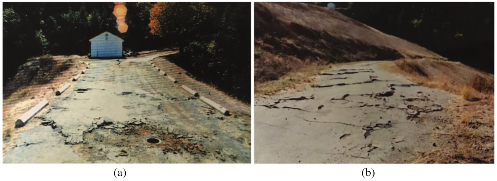
Cracking of Austrian dam after the 1989 Loma Prieta earthquake. (a) Longitudinal and transverse cracking on the dam crest near the left abutment and (b) cracking along access road on the lower portion of the downstream face (Boulanger, 2019).

Out of the 94 case histories, the number of cases that are classified as none, minor, moderate, severe, and collapse are 15, 49, 19, 8, and 3, respectively. Because there are only 3 case histories that are assigned to the collapse damage state, we do not develop a capacity model for collapse. The data used for assigning damage states to each dam and an explanation of the assignment have been compiled and are published as an electronic dataset in the DesignSafe Data Depot data repository (He and Rathje, 2023). The dataset provides the dam’s name, location, RS, earthquake event, damage description source, and the assigned damage state for this study.

Proposed seismic capacity relationships

A probabilistic seismic capacity relationship can be written as:

P_{DS} (RS) = Φ [\frac{\ln (RS) - μ_{\ln C}}{σ_{\ln C}}],

(13)

where $P_{DS} (RS)$ is the probability that the damage state ( $DS$ ) is exceeded given a value of $RS$ , $Φ [\cdot]$ is the standard normal cumulative distribution function, and $μ_{\ln C}$ and $σ_{\ln C}$ are the mean and standard deviation (in natural log units) of the EDP for the capacity relationship for a specific damage state.

Porter et al. (2007) provide a summary of different approaches that can be used to construct seismic capacity relationships. For this study, we use the procedure that is based on the method for bounding EDP. This approach is appropriate when you have failed and un-failed specimens, and the peak EDP is known for each specimen. Porter et al. (2007) suggest performing a least-square fit to the binary failure data to fit a fragility function to the bounding-EDP data. To apply this approach, the case history data points are grouped into bins of $RS$ , where each bin has the same width in log space. Next, the fraction of observations in each $RS$ bin that experienced the damage state (or larger) is calculated, along with the average $RS$ for each bin. These values serve as independent data points (bin-average data points) of the probability of the damage state and the $RS$ . Finally, a least-squares fit is performed to these data points using Equation 13 to obtain the values of $μ_{\ln C}$ and $σ_{\ln C}$ .

Figure 6 shows the resulting capacity relationships derived for each damage state. The red points represent the observed values of $RS$ and are plotted at a probability of either 1 or 0 based on whether the dam experienced the associated damage state (or higher) or not. The black points represent the fraction of observations in each $RS$ bin with $P_{DS}$ = 1 and these points are used in the least-squares fit. The resulting values of $μ_{\ln C}$ and $σ_{\ln C}$ for each damage state are listed in Table 2. Clearly, there is overlap in the values of the observed $RS$ for each damage state, which results in broad capacity relationships, as shown in black, with large $σ_{\ln C}$ (∼1.0, Table 2). When the capacity relationships for the three damage states are plotted together, as shown in Figure 6d, the capacity relationships shift to the right as the damage state goes from minor to severe/collapse, indicating that larger values of $RS$ are required to induce the more significant damage states. The shapes of the capacity curves are similar due to the similar values of $σ_{\ln C}$ for the three damage states.

Figure 6.

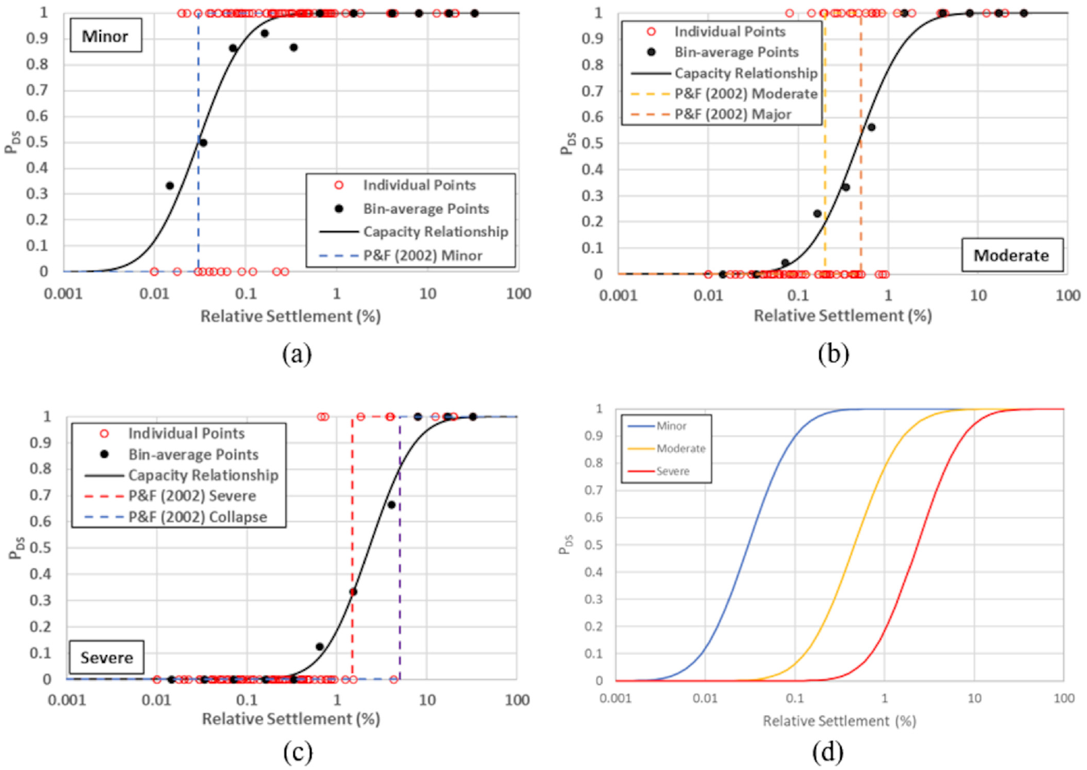
Capacity relationships developed for (a) minor, (b) moderate, (c) collapse damage states, and (d) comparison of capacity relationships for all three damage states.

Table 2.

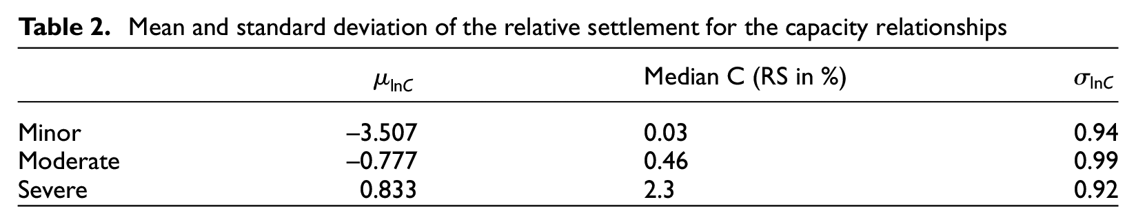
Mean and standard deviation of the relative settlement for the capacity relationships

	$μ_{\ln C}$	Median C (RS in %)	$σ_{\ln C}$
Minor	−3.507	0.03	0.94
Moderate	−0.777	0.46	0.99
Severe	0.833	2.3	0.92

Also shown in Figure 6a to c are the step function capacity relationships from Pells and Fell (2002) for their damage states. Because Pells and Fell (2002) define six damage states, the moderate and major damage states from Pells and Fell (2002) are plotted with the moderate damage state from this study, and the Pells and Fell’s (2002) severe and collapse damage states are plotted with the severe damage state from this study. The step function capacity relationships from Pells and Fell (2002) generally are located close to the median values of the developed probabilistic capacity relationships in Figure 6, indicating consistency between the previous capacity models and those developed in this study. The main difference between the proposed relationships is the shape, with the developed capacity relationships smoothly increasing with increasing RS and the Pells and Fell (2002) relationships increasing rapidly as a step function.

Example application

The development of probabilistic seismic fragility relationships is demonstrated for a hypothetical dam. This process involves developing a seismic demand relationship from numerical simulations, and combining it with the seismic capacity models to create a dam-specific fragility relationship.

The hypothetical dam (Figure 7) is a homogeneous silty sand embankment with a height of 20 m and the N_1,60 of 15 (relative density (D_r) = 57%). The reservoir water level is 16 m high, which is 80% of the dam height. The phreatic surface is assumed to be linear across the dam, and downstream the water level is at the ground surface. The side slopes are 2.5H:1V on both the upstream and downstream faces of the dam. The foundation soil thickness below the dam is 10 m and it is a sandy material with N_1,60 of 25 (D_r = 74%).

Figure 7.

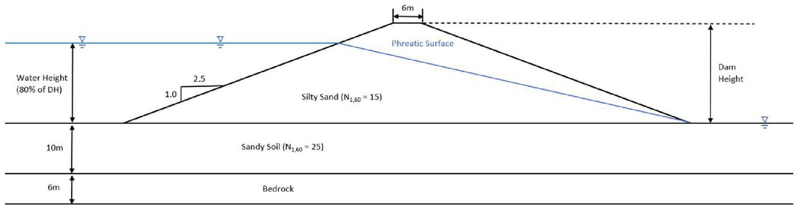
Configuration of hypothetical dam.

The seismic demand relationship is developed from the results of non-linear dynamic response analyses that use earthquake time histories from the NGA-West2 database as input for this specific dam. The fragility relationships are then developed by using Equations 7–9.

Seismic demand relationship for the hypothetical dam model

The engineering demand model predicts the median RS of the dam crest as a function of the ground motion intensity (Figure 2) as derived from the results of numerical simulations. The finite element analysis of the hypothetical dam is performed using the OpenSees analysis framework (McKenna, 1997). The constitutive models and modeling methods implemented in this study have been applied and utilized by many other researchers (e.g. Qiu and Elgamal, 2020, 2022; Wu et al., 2021). Figure 8 shows the numerical dam model built using Scientific ToolKit for OpenSees (STKO), developed by ASDEA Software. STKO is used as the pre- and post-processor for the finite element analyses in this study. The foundation layer of the model extends laterally from the dam a distance of 70 m. To model the free-field condition at the edge of the lateral boundaries, large free-field columns with increased thickness, as recommended by Zienkiewicz et al. (1989), are utilized to ensure a one-dimensional response. Quadrilateral FourNodeQuadUP elements (Mazzoni et al., 2006) are used throughout the model with element sizes generally 1 m high and 2 m wide in the foundation, and 0.5 m high and 0.2 to 2 m wide within the dam.

Figure 8.

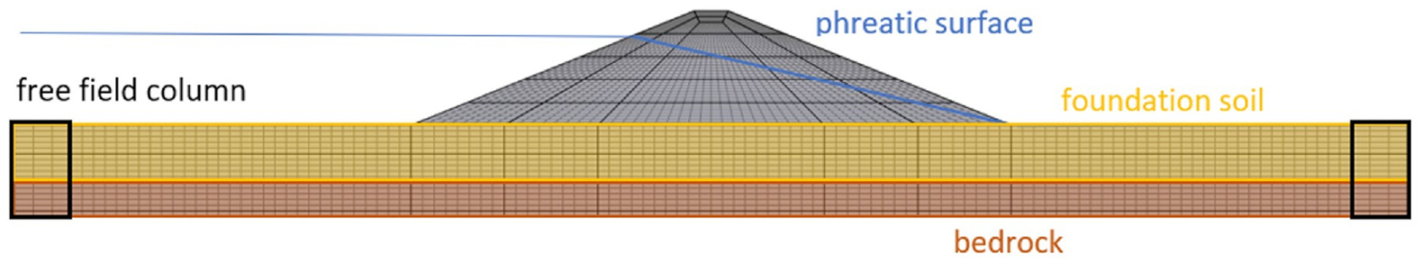
Finite element model of hypothetical dam.

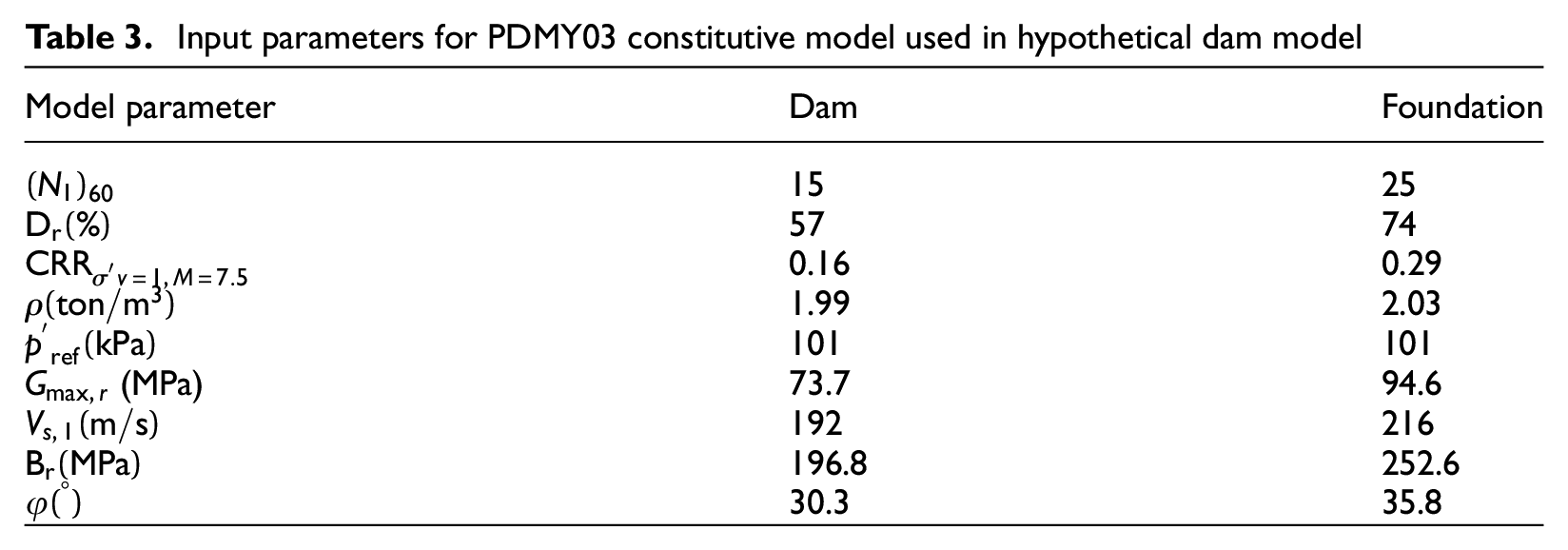
PDMY03 (Khosravifar et al., 2018) is used as the constitutive model to simulate the undrained, cyclic response of the sandy soils throughout the model. Khosravifar et al. (2018) developed a calibration that allows the PDMY03 input parameters to be assigned solely based on the D_r or standard penetration test blowcount, $(N_{1})_{60}$ , of the soil. This calibration is based on triggering liquefaction in 15 loading cycles at a cyclic stress ratio equal to $CR R_{σ^{'} v = 1, M = 7.5}$ at a vertical effective stress of 1 atm. The input parameters for PDMY03 for the $(N_{1})_{60}$ values of the dam and foundation are shown in Table 3. At the bottom of the model, the bedrock layer is modeled using the elastic isotropic material available in OpenSees, with a shear wave velocity of 760 m/s and density of 2.5 t/m³. The pore pressure degrees of freedom are fixed to zero for all the nodes that are at or above the phreatic surface.

Table 3.

Input parameters for PDMY03 constitutive model used in hypothetical dam model

Model parameter	Dam	Foundation
$(N_{1})_{60}$	15	25
$D_{r} (%)$	57	74
$CR R_{σ^{'} v = 1, M = 7.5}$	0.16	0.29
$ρ (ton / m^{3})$	1.99	2.03
${p^{'}}_{ref} (kPa)$	101	101
$G_{\max, r}$ (MPa)	73.7	94.6
$V_{s, 1} (m / s)$	192	216
$B_{r} (MPa)$	196.8	252.6
$φ (^{°})$	30.3	35.8

A suite of 32 input motions is selected from the NGA-West2 database. These motions are selected to represent ground motions from shallow crustal earthquakes from active tectonic regions, which can induce significant damage to earth dams. All the input ground motions are unscaled from their original records and are selected to ensure ground motion intensities spread evenly across the PGA–PGV domain. Details about the selected motions are provided in the electronic supplement. 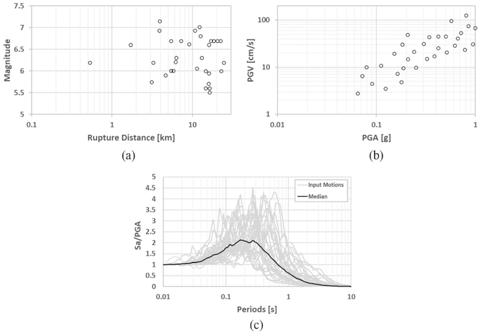Figure 9a shows a plot of moment magnitude versus rupture distance (R_rup) for the 32 input motions, in which the smallest M is 5.5 and the largest is 7.1, and R_rup varies from 0.5 to 23 km. Figure 9b shows a plot of PGA versus PGV for these motions. The largest PGA and PGV are 0.99 g and 124 cm/s, respectively. The normalized acceleration response spectra are also plotted in Figure 9c. These are a range of spectral shapes associated with the motions, and the median response spectrum peaks around a period of 0.2–0.3 s.

Figure 9.

The distribution of the 32 input motions in terms of (a) magnitude versus rupture distance, (b) PGV versus PGA, and (c) normalized acceleration response spectra.

Example simulation results are presented for the hypothetical dam subjected to the unscaled NS component of the Parkfield–Gold Hill 3W recording from the 2004 Parkfield-02, California earthquake (M = 6.0). This motion was recorded at a distance of 5.4 km, with PGA = 0.79 g and PGV = 23.2 cm/s. Figure 10a shows contour of the excess pore water pressure ratio (i.e. EPWPRatio = $r_{u} = (u / σ_{v}^{'})$ at t = 3 s, which represents the end of strong shaking as shown by the input ground motion displayed in the figure. Because the material of the dam is liquefiable and the foundation is denser and unlikely to liquefy, most of the excess pore pressure develops in the upstream face of the dam where the dam is saturated. Figure 10b and c shows displacement amplitude and y-displacement (i.e. dam settlement), respectively, at the end of strong shaking for this input motion. The largest movements occur on the upstream side of the dam due to liquefaction on the upstream side slope, especially at the shallower surface. Because the crest settlement is driven by the movement of the upstream slope, there is also more settlement on the upstream side of the crest than the downstream side, as shown in Figure 10c. The crest settlement used in the RS calculation is taken as the average vertical displacement of the left edge, center, and right edge of the dam crest. For this analysis, the crest settlement and RS are 15 cm and 0.75%, respectively.

Figure 10.

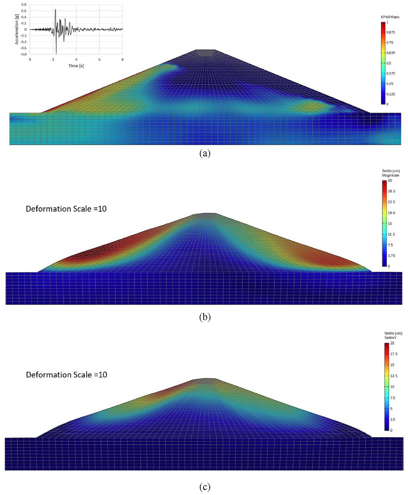
Contours of (a) excess pore pressure ratio at t = 3 s, (b) displacement magnitude at end of shaking, and (c) y-displacement settlement at end of shaking, for the hypothetical 20-m homogeneous earth dam subjected to the Parkfield–Gold Hill 3W motion with a PGA of 0.79 g.

Note that all results used for the demand model are associated with the end of shaking, and thus post-liquefaction settlement is not accounted for in the demand model. However, the settlement observations from all the case histories considered in the capacity models include any post-liquefaction settlement. The effect of ignoring the post-liquefaction reconsolidation will vary depending on the D_r of both the dam and the foundation soil, soil compressibility, and the characteristics of input motion. However, some researchers (Mehrzad et al., 2018; Zeybek and Madabhushi, 2023) have observed from centrifuge tests that, even for loose sandy materials, the post-liquefaction consolidation settlement may only be 10%–20% of the co-seismic settlement. This effect should be less for medium and dense sands. Nonetheless, the limitation of ignoring post-liquefaction reconsolidation settlement in the demand model when that mechanism of deformation is included in the capacity models should be noted.

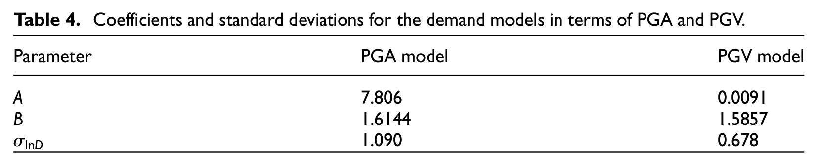
The resulting RS of the dam from each numerical analysis ranges from 0.02% to 10.8% and is plotted against the IMs of PGA and PGV in Figure 11. For each IM, the RS clearly increases with increasing intensity and a power law demand model (Equations 2 and 3) is fit to each dataset (Table 4). 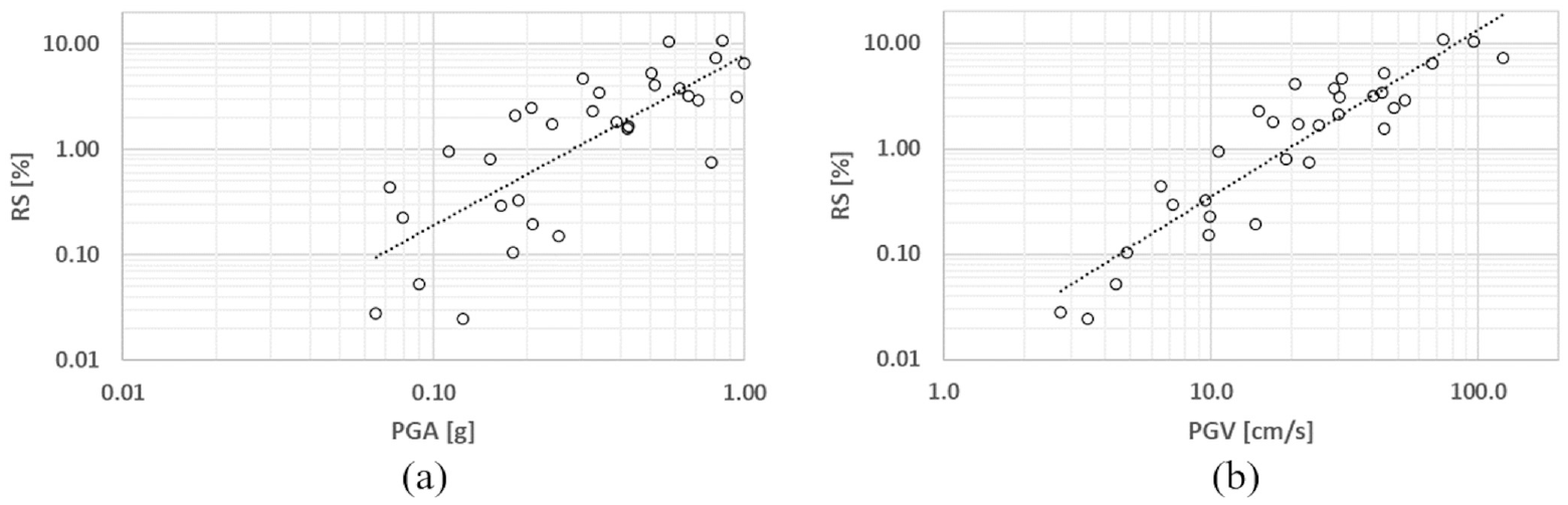Overall, the data are more scattered for the demand model using PGA as compared with the model using PGV, with $σ_{\ln D}$ 60% larger for the PGA model (Table 4).

Figure 11.

Demand models developed as a function of (a) PGA and (b) PGV for the hypothetical 20-m homogeneous earth dam and the NGA-West2 motions.

Table 4.

Coefficients and standard deviations for the demand models in terms of PGA and PGV.

Parameter	PGA model	PGV model
A	7.806	0.0091
B	1.6144	1.5857
$σ_{\ln D}$	1.090	0.678

Fragility relationships for the hypothetical dam model

With the demand models developed for the dam, fragility relationships can be derived for each damage state using Equations 7–9 with $μ_{\ln C}$ and $σ_{\ln C}$ from the capacity relationships (Table 2) for the damage state of interest and $μ_{\ln D}$ and $σ_{\ln D}$ obtained from Equation 4 and Table 4 for the IM of interest. The maximum values of PGA and PGV for the fragility curves are set to be 1.0 g and 120 cm/s, respectively, based on the maximum values of the PGA and PGV for the input motions. Fragility curves for all three damage states are created following the same procedure, but with different values of $μ_{\ln C}$ and $σ_{\ln C}$ from Table 2.

The final fragility curves for the hypothetical dam are shown in Figure 12 for the three damage states and two IMs (i.e. PGA and PGV). As expected, the fragility curves move to the right as the damage state gets more significant. At the same level of IM, the probability is larger for the lower level damage states. One may notice that the minor damage state is reached even at low levels of IM. This result may be explained by reviewing the general description of the minor damage state in the capacity model, which indicates minor damage is assigned to dams with any displacement or observed hairline cracks, even though such damage may not cause any risk to the dam.

Figure 12.

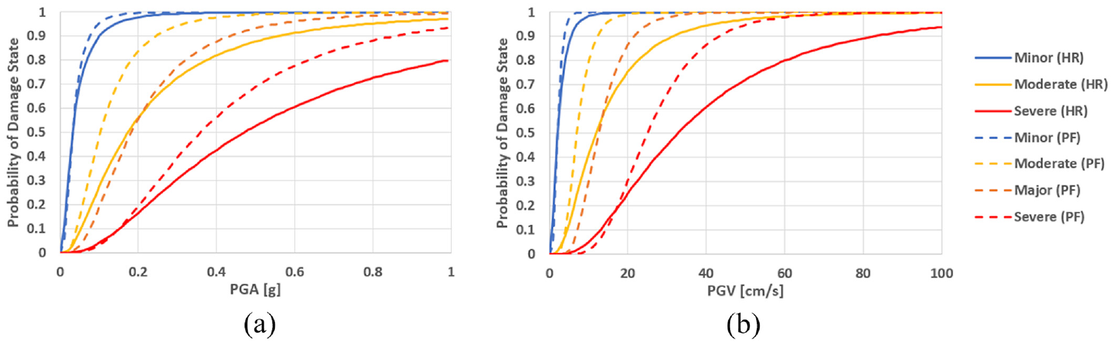
Fragility curves in terms of (a) PGA and (b) PGV for three damage states for the hypothetical 20-m homogeneous earth dam. Fragility curves derived using the capacity relationships in this study are labeled HR, while those derived using the step function capacity relationships of Pells and Fell (2002) are labeled PF.

Between the two IMs, the fragility curves developed in terms of PGA have flatter slopes when compared to the fragility curves for the same damage state for PGV. These flatter curves indicate that there is more variability in the PGA fragility curves, and it is a result of the larger $σ_{\ln D}$ for the PGA demand model (Table 4). At the maximum intensities shown in Figure 12 (PGA = 1.0 g or PGV = 100 cm/s), the probability of exceeding the minor damage state is 1.0 for both IMs. For the moderate damage state, these probabilities are about 0.95 for PGA and 1.0 for PGV, while they are 0.8 for PGA and 0.9 for PGV for the severe damage state. Given the smaller $σ_{\ln D}$ for the PGV demand model and resulting steepness of the fragility curve, the PGV fragility curves are preferred over the PGA fragility curves.

Also shown in Figure 12 are fragility curves developed using Pells and Fell (2002) capacity relationships (Figure 4) for the four of their five damage states that most closely align with those from this study. For the minor damage state, the predicted probabilities are similar for the fragility curves developed in this study and those using the Pells and Fell (2002) capacity relationships. However, the fragility curve for the Pells and Fell (2002) moderate damage state is to the left of the moderate curve from this study, while the Pells and Fell (2002) major damage fragility curve is at a similar location as the moderate damage curve from this study. These differences are associated with the different definitions of moderate damage for the two studies, and the fact that Pells and Fell (2002) defined more damage states with finer granularity, that we did not think was warranted. For the severe damage state, the fragility curve from this study is to the left of that from Pells and Fell (2002). These relative differences in the fragility curves derive directly from the differences in the locations of the capacity relationships, as shown in Figure 6.

Figure 12 also shows important differences in the shapes of the fragility curves. In general, the slopes of the fragility curves are steeper for the fragility curves derived using Pells and Fell (2002) because the Pells and Fell (2002) capacity model does not consider the variability between RS and damage state. Thus, the variability in the Pells and Fell (2002) fragility curves is associated only with the demand models. The extra variability from the proposed capacity models in this study leads to more variability in the final fragility curves. However, such variability should be taken into account to properly account for the uncertainty in the relationship between RS and damage state.

It is important to note that the seismic fragility relationships in Figure 12 are only applicable to the 20-m high dam geometry and soil conditions shown in Figure 7 and for ground motions associated with earthquakes in active crustal regions, as represented in the NGA-West2 database.

Conclusions

A probabilistic seismic fragility framework for earth dams, which is based on commonly used methods in structural earthquake engineering, is presented in this article. The framework consists of two major components: a probabilistic seismic demand model and a probabilistic seismic capacity model. The seismic demand model predicts the EDP given the ground shaking intensity and the seismic capacity model predicts the damage state given the EDP. For earth dams, the relevant EDP is the RS of the dam crest.

This article developed seismic capacity relationships for earth dams using published field observations of earth dam performance in previous earthquakes. The developed relationships are unique because the damage assessments are assigned based on the original field damage descriptions, when such descriptions are available, rather than defined by the observed EDP, RS. Seismic capacity relationships are developed for three damage states (i.e. minor, moderate, and severe), and are compared with the previously published capacity relationships of Pells and Fell (2002). The RS thresholds for the different damage states from this study are consistent with those from Pells and Fell (2002), but the newly developed capacity relationships more realistically capture the variability in the relationship between RS and the resulting damage state.

The application of the fragility framework was demonstrated by generating fragility models for a hypothetical 20-m high homogeneous earth dam in which the embankment consists of silty sand with D_r = 57% and is underlain by denser sand with D_r = 74%. A finite element model of the hypothetical dam was created in OpenSees and the PDMY03 constitutive model was used to simulate the undrained, cyclic soil response of both the dam and foundation materials. A suite of 32 earthquake ground motions from the NGA-West2 database was selected as input for the finite element analyses and the permanent displacements of the dam model were obtained for each input motion. The RS was computed for each analysis from the permanent displacements and used to develop seismic demand models, which were combined with the capacity relationships to develop the fragility models. The demand and fragility models were created as a function of different IMs (i.e. PGA and PGV) to examine the efficiency of the two different IMs. With the hypothetical dam model and selected input ground motions, PGV is more efficient in predicting RS than PGA, with the smaller $σ_{\ln D}$ , and this leads to less variability in the fragility relationships. Thus, the PGV fragility relationships are preferred over the PGA relationships to predict earthquake-induced damage to earth dams in this study.

The seismic fragility relationships in this study were derived for a single dam geometry with one set of soil conditions. Incorporating epistemic uncertainties in the dam geometry and/or soil properties would influence the demand models and the resulting fragility relationships. These uncertainties are important to incorporate, particularly when considering a poorly characterized dam or a portfolio of dams with unknown soil properties. In addition, the demand models developed in this model utilized ground motions from active crustal regions, and thus are not applicable to other tectonic regions such as subduction zones or Central and Eastern North America. However, the framework described in this article can be used to develop fragility relationships for a specific dam or for generic dam classes in any tectonic region. When utilizing the fragility framework, the seismic capacity relationships from this study are transferable to other dams and tectonic regions, but the seismic demand model must be developed from analyses of region-specific or site-specific dam geometries (e.g. height, side slopes) and characteristics (e.g. soil type, strength, core type) that utilize input motions representative of the tectonic region of interest. The proposed capacity models which relate RS to damage states based on observed dam performances also allow one to implement the PBEE framework up to damage analysis level, which is a step forward in applying PBEE in seismic dam performance analysis.

Footnotes

Declaration of conflicting interests

The author(s) declared no potential conflicts of interest with respect to the research, authorship, and/or publication of this article.

Funding

The author(s) disclosed receipt of the following financial support for the research, authorship, and/or publication of this article: This work was sponsored through funding from the State of Texas through the TexNet Seismic Monitoring Program at the Bureau of Economic Geology of the University of Texas and the Texas Division of Emergency Management (Project no. UTAUS-FA00000170). Additional funding was provided by the Janet S. Cockrell Centennial Chair in Engineering at the University of Texas.

ORCID iD

Jingwen He

Research data availability

The data used for assigning damage states to each dam and an explanation of the assignment have been published as an electronic dataset in the DesignSafe Data Depot data repository (https://doi.org/10.17603/ds2-pwtv-p173 v1).

References

Akai

Bray

Boulanger

Christian

Finn

Harder

Idriss

Ishihara

Iwasaki

Mitchell

Moriwaki

Nakagawa

O’Rourke

Seed

Sitar

Soga

Somerville

Towhata

Youd

(1995) Geotechnical Reconnaissance of the Effects of the January 17, 1995 Hyogoken-nanbu Earthquake, Japan. Berkeley, CA: Earthquake Engineering Research Center.

Ambraseys

(1960) On the seismic behavior of earth dams. In: Proceedings of the second world conference on earthquake engineering, Vol. 2, Tokyo, Japan, pp. 331–356. Available at: https://www.iitk.ac.in/nicee/wcee/article/vol.1_session5_331.pdf (accessed 20 March 2024).

Ancheta

Darragh

Stewart

Silva

Chiou

Wooddell

Graves

Kottke

Boore

Kishida

Donahue

(2014) NGA-West2 database. Earthquake Spectra 30(3): 989–1005.

Boulanger

(2019) Nonlinear dynamic analyses of Austrian dam in the 1989 Loma Prieta earthquake. Journal of Geotechnical and Geoenvironmental Engineering 145(11). DOI: 10.1061/(ASCE)GT.1943-5606.0002156.

Celik

Ellingwood

(2010) Seismic fragilities for non—ductile reinforced concrete frames—Role of aleatoric and epistemic uncertainties. Structural Safety 32(1): 1–32.

Chen

Jin

Zhou

Wang

(2009) Investigation and analysis on earthquake damages to reservoirs in Zhongjiang county during Ms 8.0 Wenchuan earthquake J. J. Catastrophology 24(3): 69–74.

Cornell

Jalayer

Hamburger

Foutch

(2002) Probabilistic basis for 2000 SAC federal emergency management agency steel moment frame guidelines. Journal of Structural Engineering 128(4): 526–533.

Fell

Bowles

Anderson

Bell

(2000) The status of methods for estimation of the probability of failure of dams for use in quantitative risk assessment. Transactions of the International Congress on Large Dams 1: 213–236.

Franke

Kramer

(2014) Procedure for the empirical evaluation of lateral spread displacement hazard curves. Journal of Geotechnical and Geoenvironmental Engineering, 140(1): 110–120.

10.

Fraser

Wald

Lin

K-W

(2008) Using ShakeMap and ShakeCast to prioritize post-earthquake dam inspections. Geotechnical Earthquake Engineering and Soil DynamicsIV: 1–10. https://doi.org/10.1061/40975(318)183

11.

Harder

Kayen

Kelson

Kishida

(2011) Preliminary Observations of the Fujinuma Dam Failure Following the March 11, 2011 Tohoku Offshore Earthquake, Japan. Berkeley, CA: Geotechnical Extreme Events Reconnaissance Report No. GEER-25e.

12.

Harder

Bray

Volpe

Rodda

(1998) Performance of Earth Dams during the Loma Prieta Earthquake. Washington, DC: U.S. Geological Survey Professional Paper 1552-D.

13.

Rathje

(2023) Database for the Development of Capacity Relationships for Earth Dam. (DesignSafe-CI). https://doi.org/10.17603/ds2-pwtv-p173 v1

14.

Kennedy

Ravindra

(1984) Seismic fragilities for nuclear power plant risk studies. Nuclear Engineering and Design 79(1): 47–68.

15.

Khosravifar

Elgamal

(2018) A 3D model for earthquake-induced liquefaction triggering and post-liquefaction response. Soil Dynamics and Earthquake Engineering 110: 43–52.

16.

Khosravikia

Kurkowski

Clayton

(2020) Fragility of masonry veneers to human-induced central U.S. earthquakes using neural network models. Journal of Building Engineering 28: 101100. https://doi.org/10.1016/j.jobe.2019.101100

17.

Kramer

(2008) Performance-based earthquake engineering: Opportunities and implications for geotechnical engineering practice. Geotechnical Earthquake Engineering and Soil DynamicsIV: 1–32. https://doi.org/10.1061/40975(318)213

18.

McKenna

(1997) Object-oriented Finite Element Programming: Frame-works for Analysis, Algorithms and Parallel Computing. Berkeley, CA: Department of Civil Engineering, University of California, Berkeley.

19.

Mazzoni

McKenna

Scott

Fenves

(2006) OpenSees command language manual. Pacific Earthquake Engineering Research (PEER) Center 264(1): 137–158.

20.

Mehrzad

Jafarian

Lee

Haddad

(2018) Centrifuge study into the effect of liquefaction extent on permanent settlement and seismic response of shallow foundations. Soils and Foundations 58(1): 228–240.

21.

Moehle

Deierlein

(2004) A framework methodology for performance-based earthquake engineering. In: 13th world conference on earthquake engineering, paper no. 679, p. 12. WCEE Vancouver. Available at: https://www.iitk.ac.in/nicee/wcee/article/13_679.pdf (accessed 20 March 2024).

22.

Nielson

DesRoches

(2007) Analytical seismic fragility curves for typical bridges in the Central and Southeastern United States. Earthquake Spectra 23(3): 615–633.

23.

Padgett

DesRoches

(2008) Methodology for development of analytical fragility curves for retrofitted bridges. Earthquake Engineering and Structural Dynamics 37(8): 1157–1174.

24.

Pang

Zou

Kong

(2019) Seismic performance assessment of high CFRDs based on fragility analysis. Science China Technological Sciences 62: 635–648.

25.

Pells

Fell

(2002) Damage and Cracking of Embankment Dams by Earthquakes and the Implications for Internal Erosion and Piping. Sydney, NSW, Australia: School of Civil and Environmental Engineering, The University of New South Wales.

26.

Porter

Kennedy

Bachman

(2007) Creating fragility functions for performance-based earthquake engineering. Earthquake Spectra 23(2): 471–489. https://doi.org/10.1193/1.2720892.

27.

Qiu

Elgamal

(2020) Numerical simulations of LEAP centrifuge tests for seismic response of liquefiable sloping ground. Soil Dynamics and Earthquake Engineering 139: 106378. https://doi.org/10.1016/j.soildyn.2020.106378

28.

Qiu

Elgamal

(2022) Numerical simulations of LEAP centrifuge experiments using a multi-surface cyclic plasticity sand model. In: Conference on performance-based design in earthquake geotechnical engineering, pp. 1812–1820. Available at: https://link.springer.com/chapter/10.1007/978-3-031-11898-2_164 (accessed 20 March 2024).

29.

Ramanathan

(2012) Next Generation Seismic Fragility Curves for California Bridges Incorporating the Evolution in Seismic Design Philosophy. Atlanta, GA: Georgia Institute of Technology.

30.

Rathje

(2022) A seismic fragility framework for earth dams. In: Lifelines 2022, Los Angeles, CA, pp. 405–415. Available at: https://doi.org/10.1061/9780784484432.036 (accessed 20 March 2024).

31.

Rathje

Saygili

(2008) Probabilistic seismic hazard analysis for the sliding displacement of slopes: Scalar and vector approaches. Journal of Geotechnical and Geoenvironmental Engineering, 134(6): 804–814.

32.

Regina

Zimmaro

Ziotopoulou

Cairo

(2023) Evaluation of the optimal ground motion intensity measure in the prediction of the seismic vulnerability of earth dams. Earthquake Spectra 39: 2352–2378. https://doi.org/10.1177/87552930231170894

33.

Seed

Makdisi

De Alba

(1978) The performance of earth dams during earthquakes. Journal of the Geotechnical Engineering Division 104(7): 967–994.

34.

Seed

Dickenson

Riemer

Bray

Sitar

Mitchell

Power

(1990) Preliminary Report on the Principal Geotechnical Aspects of the October 17, 1989 Loma Prieta Earthquake. Berkeley, CA: Earthquake Engineering Research Center.

35.

Swaisgood

(2003) Embankment dam deformations caused by earthquakes. In: 2003 pacific conference on earthquake engineering, Paper Number 014. Available at: https://www.nzsee.org.nz/db/2003/View/Paper014s.pdf (accessed 20 March 2024).

36.

Swaisgood

(1998) Seismically-induced deformation of embankment dams. In: Proceedings of sixth national conference on earthquake engineering, Seattle, WA, 31 May–4 June.

37.

U.S. Army Corps of Engineers: Federal Emergency Management Agency (2020) National Inventory of Dams. Available at: https://nid.sec.usace.army.mil/ (accessed 20 March 2024).

38.

U.S. Committee on Large Dams (USCOLD) (2000) Observed Performance of Dams during Earthquakes Volume II. Denver, CO: U.S. Committee on Large Dams.

39.

U.S. Committee on Large Dams (USCOLD) (2014) Observed Performance of Dams during Earthquakes Volume III. Denver, CO: U.S. Committee on Large Dams.

40.

D-Q

Liu

(2021) Seismic performance of earth dams founded on liquefiable soil layer subjected to near-fault pulse-like ground motions. Soil Dynamics and Earthquake Engineering 143: 106623. https://doi.org/10.1016/j.soildyn.2021.106623

41.

Yan

(1991) Seismic Deformation Analysis of Earth Dams: A Simplified Method. Pasadena, CA: California Institute of Technology.

42.

Yang

(2021) Calibrated Fragility Functions for Seismic Loading of Sacramento-San Joaquin River Delta Levees. Los Angeles, CA: Civil and Environmental Engineering, University of California, Los Angeles.

43.

Zeybek

Madabhushi

(2023) Assessment of soil parameters during post-liquefaction reconsolidation of loose sand. Soil Dynamics and Earthquake Engineering 164: 107611. https://doi.org/10.1016/j.soildyn.2022.107611

44.

Zienkiewicz

Bicanic

Shen

(1989) Earthquake input definition and the transmitting boundary conditions. In: Doltsinis

(ed.) Advances in Computational Nonlinear Mechanics. Berlin: Springer-Verlag, pp. 109–138.

Seismic capacity models for earth dams and their use in developing fragility curves

Abstract

Keywords

Introduction

Seismic fragility framework

Probabilistic seismic demand model

Probabilistic seismic capacity model

Probabilistic fragility relationship

Previous studies on seismic dam fragilities

Development of seismic capacity model for earth dams

Damage assessment of earth dams

Previous capacity models

Development of database for observed earth dam performance

Proposed seismic capacity relationships

Example application

Seismic demand relationship for the hypothetical dam model

Fragility relationships for the hypothetical dam model

Conclusions

Footnotes

Declaration of conflicting interests

Funding

ORCID iD

Research data availability

References