Sage Journals: Discover world-class research

Abstract

This study assesses the variability of shear-wave (V_S) profile determinations for a suite of methods at six industrial sites. The methods include active, consisting of multi-channel analysis of surface waves (MASW), as well as passive, consisting of refraction microtremor (ReMi), and extended spatial autocorrelation (ESAC). The purpose is to ascertain the effect of the higher level of ambient noise on the results from the different methods, as only a few of these many methods are commonly used for site characterization. The measured dispersion curves are in fair agreement with one another. The average coefficient of variation (CoV; the percentage ratio of the standard deviation to the mean) for the dispersion curves varied from 2.5% to 12.6%. In contrast, over the V_S-depth domain, the average shear-wave velocity profiles to a depth z (V_S,Z) vary from 11.6% to 16.5% between the various methods at the different sites. This indicates that the variance among the individual methods can lead to significant misinterpretation of the shallow subsurface, while the average V_S,Z is much more robust. This reaffirms its use (mainly as V_S,30) in building codes and within ground motion prediction equations (GMPEs). At all six sites, because of inversion processes, the variability within each method ranges from 4% up to 14%. There is no correlation between the test type and the CoV. Our study focused on surface-wave measurements in noisy industrial environments, where the signals processed are typically complex. Despite this complexity, our results suggest that such tests are also applicable to industrial zones, where the noisy environment constitutes an energy source.

Keywords

MASW ESAC ReMi uncertainties

Introduction

Background

Shear-wave velocity (V_S) is commonly used to calculate the expected ground motion and predict earthquake damage (e.g. Boore, 2006; Horike, 1996; Moss, 2008). Thus, an in situ survey of V_S is one of the most crucial measurements for earthquake-related geotechnical engineering. Shear-wave velocity directly correlates with the rigidity or stiffness of the material, expressed by the elastic shear modulus (G). Therefore, V_S, as a proxy for G, is widely used in construction, engineering, and seismic response studies. Hence, the accuracy of a test and its proper interpretation are critical to reliable estimation of resistance to shaking.

The leading quantitative measure of a site is V_S,30—the time-averaged shear-wave velocity in the top 30 m (reviewed by Kamai et al., 2018). This index is a common predictor of site response for engineering and, therefore, is used in seismic building codes, such as the European Committee for Standardization (2004) and National Earthquake Hazards Reduction Program (NEHRP) provisions (Building Seismic Safety Council, 1997). The V_S,30 is also often used in ground motion prediction equations (GMPEs) as an index for site characterization and micro-zonation (e.g. Abrahamson and Silva, 2008; Kamai et al., 2016).

The V_S profiles are constrained using geophysical methods, divided into two main categories: invasive or non-invasive. Invasive methods involve the assessment of V_S from a borehole, using several types of measurements, such as down-hole (DH) measurements and cross-hole seismic testing. Non-invasive methods include active and passive determination of V_S. Techniques used include reflection, refraction, refraction microtremor (ReMi), multi-channel analysis of surface waves (MASW), extended spatial autocorrelation (ESAC), horizontal-to-vertical spectral ratio (HVSR), and so on. Invasive methods generally provide sufficient resolution as a function of depth and are considered more reliable than non-invasive methods (Garofalo et al., 2016a). However, invasive tests require drilling at least one expensive borehole, while non-invasive methods are environmentally friendly, low cost, robust, and provide reliable V_S,30 data (Xia et al., 2002). Therefore, non-invasive tests are more common, while invasive tests are usually adopted in projects of primary importance.

According to Boore (2006), there are differences between the methods, and no single method is the best for all circumstances. Thus, the use of several different tests is worthwhile for providing constrained V_S estimates; otherwise, the outcome of a series of V_S profiles has inherent and unknown uncertainties clouding the final result. Assessments of such uncertainties, which are part of the site-response analysis, are critical for probabilistic seismic hazard analysis (e.g. Bazzurro and Cornell, 2004; Rathje et al., 2010). The uncertainty can be related to various stages in the analysis, such as measurement, processing, and interpretation of the V_S profile, choice of nonlinear properties or model type, or the framework of analysis (Kamai et al., 2018).

Xia et al. (2002), compared MASW V_S profiles to direct borehole measurements at three sites. They found that the difference between them was random, ∼15% or less. Boore and Asten (2008) compared shear-wave slowness at six sites using blind interpretations of data from invasive and non-invasive methods. The slownesses from the various methods appear sufficiently alike, so that site amplifications are within about 10%–20% of those from other models. Fourteen teams of experts made a broad comparison of three different test sites (InterPacific Project, Garofalo et al., 2016a). They concluded that the variability in the shear-wave velocity profiles is similar for both invasive and non-invasive methods. This is despite the higher resolution at each depth provided by the former.

The estimation of the V_S profile in areas subject to environmental noise, such as in industrial areas, near roads, and in cities, is more challenging. This is due to the random (often stationary) broadband noise sources from machines, cars, trucks, pumps, buildings, and so on. The contribution of this random noise can be significant to the V_S assessment, especially for the lower frequencies propagating deeper into the section investigated. For certain passive tests, without knowing the noise source locations, it can be challenging to extract the dispersion curve and properly estimate V_S. For active tests at such sites, the background noise can mask the surface-wave signal generated by the active source (usually a sledgehammer) and degrade the results, especially in the far field.

In this study, I focus on six sites (Figures 1 and 2). I estimate the uncertainties associated with measuring and interpreting the near-surface V_S profile in challenging environments, where random or continuous sources of noise dominate the wave field. I a priori assume that at these types of sites, the V_S profile uncertainties can be more significant, and the active methods will probably be less reliable, especially in the far field that involves a deeper section.

Figure 1.

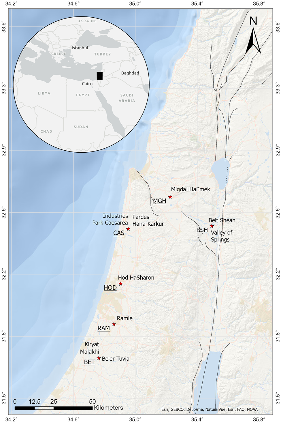
Location map with the main active faults of the area (faults modified after Hamiel et al., 2018; Hofstetter et al., 1996; Kagan et al., 2011; Sharon et al., 2020).

Figure 2.

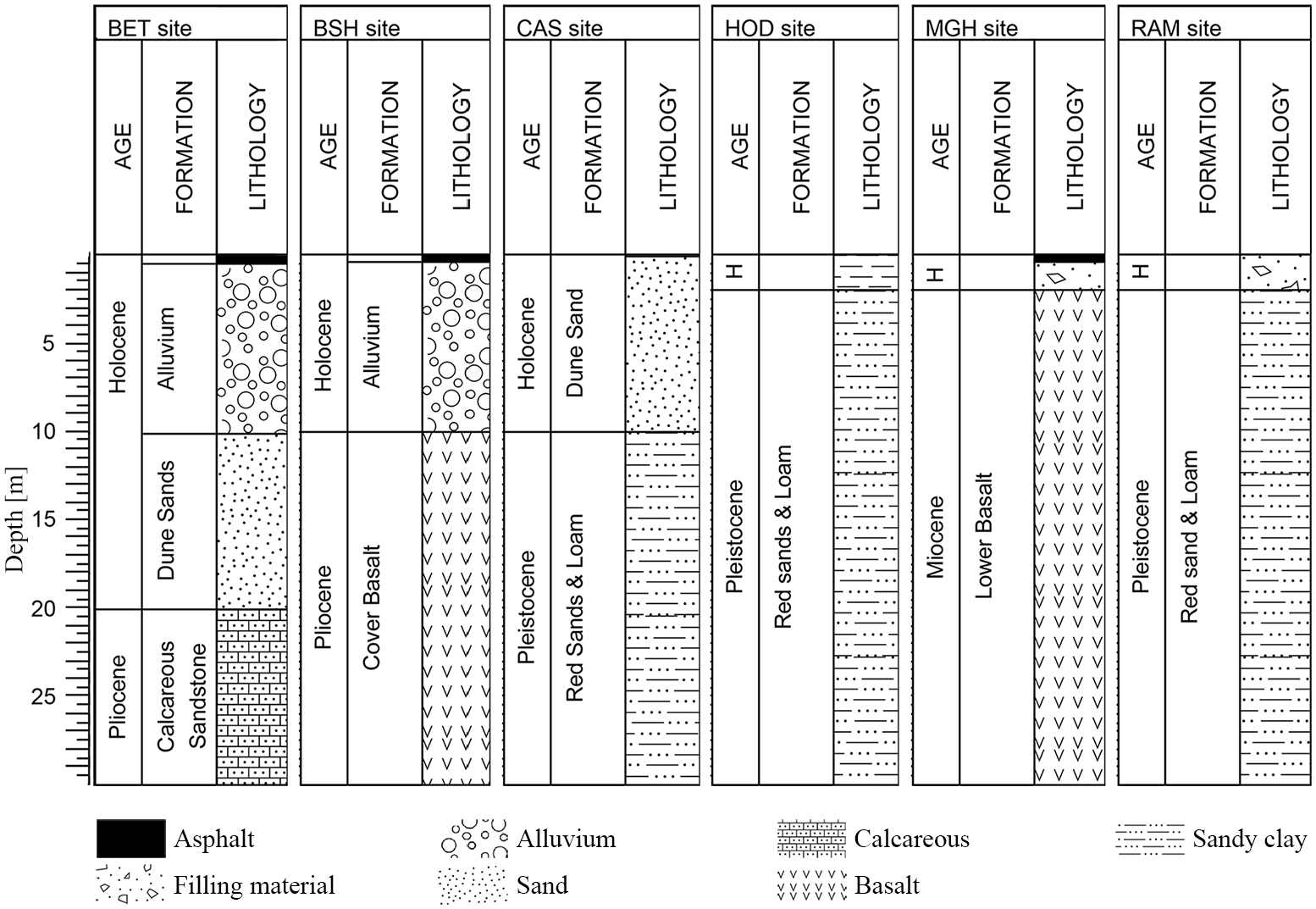
Schematic columnar section of the six sites (H for Holocene).

Site conditions and geological setting

The BET site is located near the town of Kiryat Malakhi inside the industrial area of Be’er Tuvia (Figure 1 and Supplemental Figure A1). The data were acquired near the Local Council of Be’er Tuvia, over a thin asphalt layer on top of Holocene alluvium. The Holocene Dune Sands and the Pliocene Calcareous Sandstone Units are assumed to comprise the upper tens of meters beneath the surface (Sneh and Rosensaft, 2004) (Figure 2). The BSH site is located near the city of Beit Shean within the Shan factories zone in the Valley of Springs (Figure 1 and Supplemental Figure A4). The data were acquired near a cooling facility where a thin asphalt layer overlies several tens of meters of the Holocene alluvium, underlain by the Pliocene Cover Basalt Unit (Hatzor, 2000) (Figure 2). The CAS site is located near the community of Pardes Hana-Karkur inside the Industries Park Caesarea (Figure 1 and Supplemental Figure A7). The data were acquired over the Holocene Dune Sand Unit underlain by the Pliocene Red Sands & Loam Unit (Sneh and Rosensaft, 2004) (Figure 2). The HOD site is located within the town of Hod Hasharon (Figure 1 and Supplemental Figure A10). The data were acquired near the community’s Local Council over rich clay soil. The Pleistocene Red Sand & Loam Unit is assumed to comprise the uppermost 10 m beneath the surface (Sneh and Rosensaft, 2008) (Figure 2). The MGH site is located near the town of Migdal HaEmek inside the industrial zone (Figure 1 and Supplemental Figure A13). The data were acquired inside the Sunfrost factory over a thin asphalt layer on top of up to a meter of artificial fill. Weathered basalt is exposed under the filling material (Figure 2). The RAM site is located in the western part of the city of Ramle, adjacent to a water reservoir belonging to Mekorot (Israel’s national water company) (Figure 1 and Supplemental Figure A16). The data were acquired near the reservoir over a thin layer of artificial gravel on top of the Pliocene Red Sand and Loam Unit (Sneh and Rosensaft, 2004) (Figure 2).

Seismic methods

Surface-wave propagation occurs at free boundaries, such as the surface of the earth. In a layered medium, surface-wave propagation is ruled by geometric dispersion, in which longer wavelengths penetrate to greater depths. Therefore, at each frequency, the phase velocity depends on the properties of the examined interval below the subsurface (Garofalo et al., 2016a). The wave equation has multiple solutions at given frequencies or wavenumbers, which explains the multi-modal character of surface wave dispersion. Therefore, in a layered medium, the surface-wave propagation can be a multi-modal phenomenon, where different modes can exist at the same frequency but with different propagation velocities (Foti, 2000). The phase velocity depends primarily on the shear-wave velocity and is relatively insensitive to realistic variations in density and compressional wave velocity with depth (Nolet, 1981). Therefore, the surface wave velocity is a reasonable indicator of V_S (Park et al., 1999).

Most surface-wave methods are based on three main steps: (1) acquisition of experimental data, (2) signal processing to obtain the experimental dispersion curve, and (3) one-dimensional (1D) inversion to estimate V_S (e.g. Dal Moro, 2014; Foti et al., 2014). It is worth emphasizing that the fundamental mode of surface waves is assumed to dominate the recorded wavefield, and higher modes can be ignored (Park et al., 1998). This assumption can be accepted in cases where the dispersive profile consists of velocity increasing with depth, with no strong impedance contrasts. However, in reality, higher modes are generated in most cases and can possess significant fractions of the energy (Gucunski and Woods, 1991; Stokoe et al., 1994). Therefore, failure to separate the different modes can lead to erroneous results.

In this research, I used MASW (Park et al., 1999) to acquire both the vertical and the radial components of Rayleigh waves and the transverse component of Love waves (by Dal Moro’s notation (2014): ZVF, RVF, and THF, respectively (Figure 3). To provide better estimations, I attempted to resolve the different modes. I also acquired data from the ESAC (Ohori et al., 2002) and the ReMi (Louie, 2001) methods. These surface-wave methods are commonly divided into two main groups (Table 1): active methods, where the source of the seismic waves can be a sledgehammer or an accelerated weight, versus passive methods in which the source is uncontrolled. Thus the waves are the result of spatially random sources.

Figure 3.

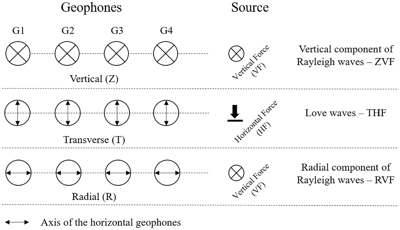
Schematic plan of sources and geophones orientation to obtain different surface-wave components (modified after Dal Moro, 2014).

Table 1.

Acquisition parameters

Method	Source andimpactdirection	Stacking	Samplinginterval (ms)	Recordlength	Number ofgeophones	Geophonesinterval (m)	Length of the line (m)
ZVF (MASW)	8 kg sledgehammerstriking vertically	3–5	0.125	0.5–2 (s)	12–24	3–5	33–92
RVF (MASW)	8 kg sledgehammerstriking vertically
THF (MASW)	8 kg sledgehammerstriking horizontally
ReMi	Ambient noise	−	2	25–30 (min)
ESAC	Ambient noise	−	2	25–30 (min)	24–48

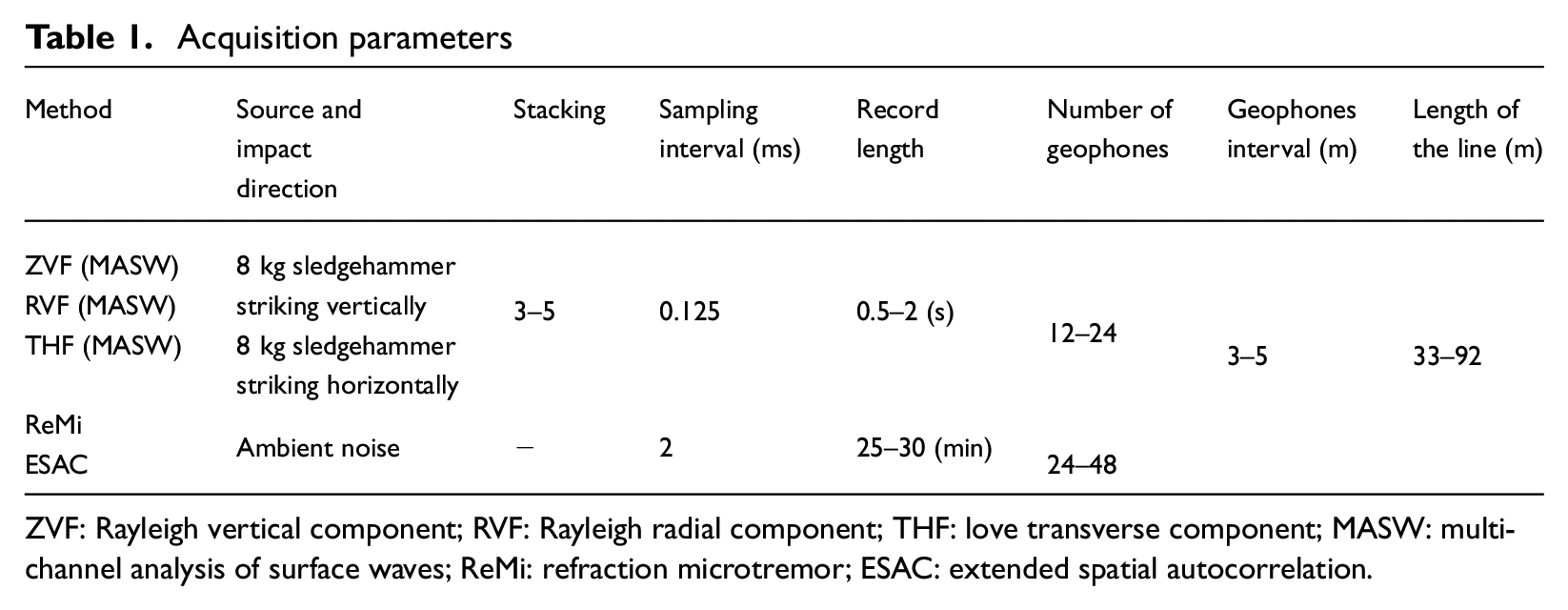
ZVF: Rayleigh vertical component; RVF: Rayleigh radial component; THF: love transverse component; MASW: multi-channel analysis of surface waves; ReMi: refraction microtremor; ESAC: extended spatial autocorrelation.

To calculate which frequencies bias each site, and if there are preferential directions to the noise in the wavefield, and how these noise properties vary with time, I used the HVSR. HVSR is based on measuring two horizontal and one vertical component at a single station. By comparing the Fourier spectrum of the average horizontal components to its vertical component, the fundamental frequency of the site can be defined. Over the last decades, methods using a single station to record environmental noise have provided promising results in estimating HVSR (e.g. Arai and Tokimatsu, 2004; Bard, 1998; Mucciarelli and Gallipoli, 2001).

By acquiring HVSR data, we can also produce: (1) a time-dependent spectrogram; (2) power spectral density curves, which are the signal’s power content versus frequency; and (3) HVSR directivity.

Acquisition

In this research, both active and passive surface wave data were collected by adopting an “L”-shaped array (Dal Moro, 2014) (Figure 4). This shape allows us to acquire five different types of data sets using vertical geophones: ZVF and ReMi for each array line segment (a total of four data sets) and ESAC from both line segments. By changing to horizontal geophones (identical cable layout) adequately oriented for RVF (and then reoriented for THF), I acquire four more data sets for both line segments. Ideally, this “L” array provides nine different types of data sets with minimum logistics. In practice, not all nine data sets were recorded due to limitations in time, logistics, and equipment. I used R.T. Clark’s 4.5 Hz horizontal and vertical geophones, and the data were recorded on a Geometrics Geode seismograph (Table 1). HVSR measurements were acquired for periods of 30–60 min by Gemini 2 Hz, three-component geophones.

Figure 4.

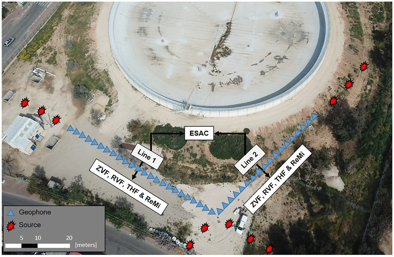
“L”-shaped array (the Ramle site).

Active survey

The active surveys were designed to acquire both Rayleigh (ZVF and RVF) and Love (THF) wave data. Measurements were collected by a linear array of geophones (Table 1), uniformly spaced according to the resolution required, and the desired depth of investigation (Socco and Strobbia, 2004). For a seismic source, I used an 8-kg sledgehammer which is commonly used and might contribute to uncertainties in an urban environment (due to the stiffness of the top layers and the urban seismic activity, the data is less clear at greater depths). For the collection of Rayleigh wave data, I used a linear array of alternating vertical and horizontal geophones. The vertical component of Rayleigh waves (ZVF) was recorded with the vertical geophones, and the radial component (RVF) with horizontal geophones oriented parallel to their linear segment. In both cases, the hammer struck vertically on a 20-cm² aluminum plate. The data logger is triggered by the closure of a circuit between the hammer and the plate. Then, the plate was moved to the next place of impact. Rotating each horizontal geophone by 90 degrees (to be oriented perpendicular to the trend of that survey line) and striking horizontally allows the acquisition of Love wave data (THF). The horizontal blows were produced by striking the end of a wooden beam, aligned perpendicular to each array, anchored by the weight of a field vehicle, or using the U.S Geological Survey’s shear-wave seismic source (Haines, 2007). For an acceptable signal-to-noise ratio, I used the so-called “vertical stacking” approach, which is a synchronized summation of multiple blows of the hammer (Table 1). I recorded the data for 0.5–2 s according to the site conditions. At each site, 3–6 offsets were selected for each data set. This gave the option of picking the dispersion curve over the clearest dispersion image.

Passive surveys

ReMi data sets were obtained passively, using the same linear array as was used for the vertical component of the Rayleigh wave (ZVF) (part of the active MASW method). ESAC data sets were simultaneously recorded on both arms of the “L”-shaped array, which included 24–48 vertical geophones. For both passive methods, field data were collected for much longer times (25–30 min) (Table 1).

Processing

The surface-wave analysis focuses on the interpretation of the experimental dispersion curve, which is used for the inversion process. The processing technique is based on the transformation of the experimental data from the time-space domain to the velocity-frequency domain. The different data sets were processed in the WinMASW® Academy software by Eliosoft by following these steps: (1) inputting the geometry of each data set (array origin coordinates, source offset, and receiver spacing). (2) For the active data sets, removing the non-relevant sections (first arrivals, coda—signals arriving after the surface waves, etc.). For the passive data sets, choosing a window length (typically 10 s). (3) For both active and passive data sets, calculating the dispersion image (Figure 5). (4) Inspecting the dispersion images from the various offsets, and picking the fundamental mode (and higher modes if they exist within the MASW data sets) at the maximum energy. In the ReMi technique (linear array), the dispersion curve is picked along the lower velocity bound (which is subjective), rather than at the maximum energy (Figure 5). (5) For each type of data set, constructed in shear wave velocity/layer thickness space, an initial model and search space is defined according to the dispersion curve. (6) Finding by the inversion process (described below), the mean V_S model and its standard deviation by means of a statistical approach based on the estimation of the marginal posterior probability density (MPPD) (Dal Moro et al., 2007).

Figure 5.

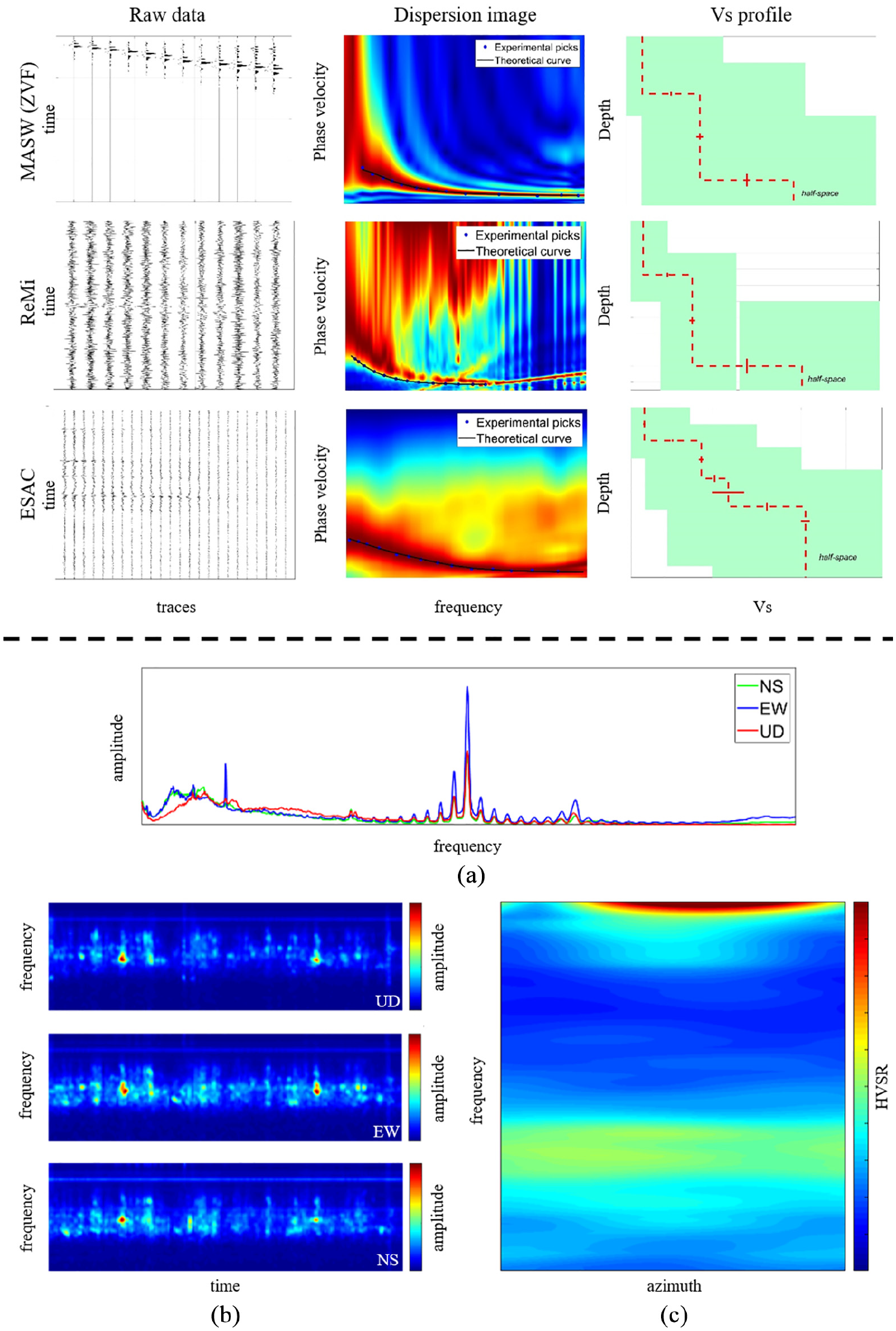
Example of data processing (results from Be’er Tuvia (BET)). In the upper section: the first column is the raw signal. The second column is the dispersion image after transformation from the time-distance domain. The third column is the marginal posterior probability density (MPPD) (Dal Moro et al., 2007), which is defined as the mean shear-wave profile. The green areas represent the model boundary. In the lower section is the “noise” analysis: A—amplitude spectrum, B—spectrograms for each component, and C—HVSR directivity.

“Noise” analysis was also processed by the WinMASW® Academy software. Amplitude spectra and spectrograms were calculated for each component (east-west, north-south, and up-down) (Figures 5A, 5B and in Supplemental material). The field experiment and the parameters of calculation of the azimuthal HVSR followed the recommendations of the site effects assessment using ambient excitations (SESAME) consortium (Bard et al., 2004) (Figure 5C and in Supplemental material).

Inversion

In the WinMASW® Academy software, the automatic inversion is conducted via genetic algorithms (Dal Moro et al., 2007). The parameterization of the model is based on the assumption of a 1D layered model consisting of a stack of homogeneous linear elastic layers over a half-space. Each layer is characterized by its thickness (except for the half-space), density, and two of the three following elastic properties: the shear-wave velocity, P-wave velocity, and Poisson’s ratio. The unknown model parameters of primary interest for our purpose are the thickness and V_S of each layer. Hence, we need to predefine either the P-wave velocity or Poisson’s ratio. Surface-wave dispersion depends strongly on the shear stiffness of the subsoil, less so on the bulk stiffness, and negligibly on the density (Garofalo et al., 2016a). Since prior information regarding saturated sediments within the depths of investigation was not available, I used realistic Poisson’s ratios for unsaturated sediments of 0.25–0.35 and realistic densities of 1.9–2.2 (g/cm³). Therefore, these parameters do not contribute significantly to the uncertainty. All V_S profiles were extracted with a minimum number of layers while keeping the misfit, that is, the discrepancy between the observed and the calculated values of the dispersion curves as low as possible.

Results

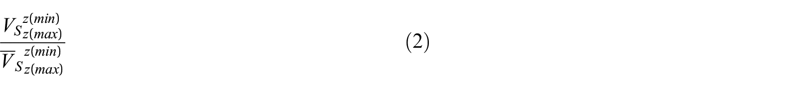
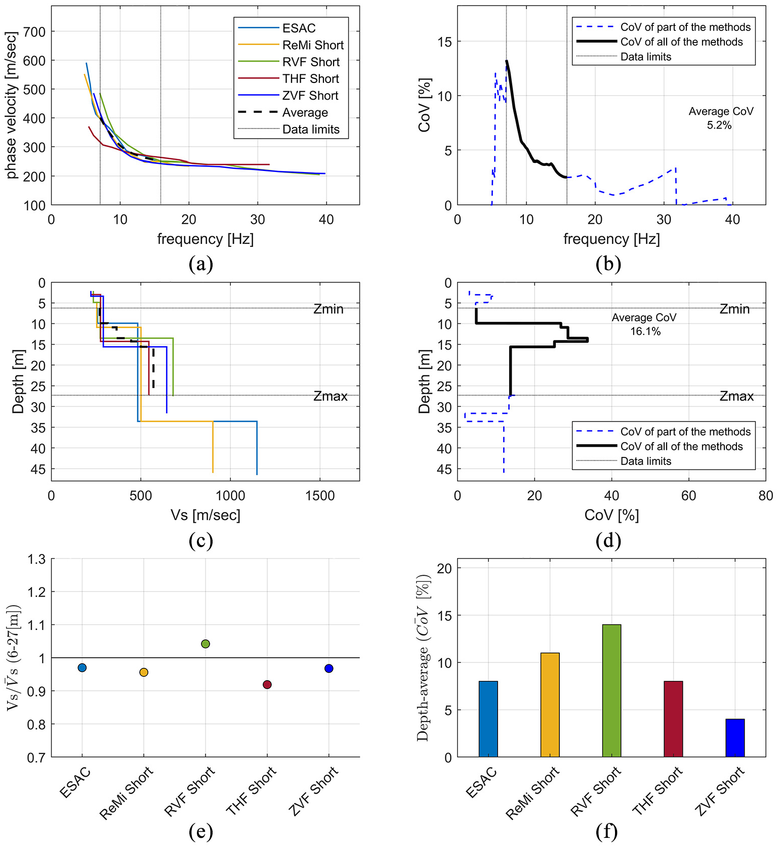
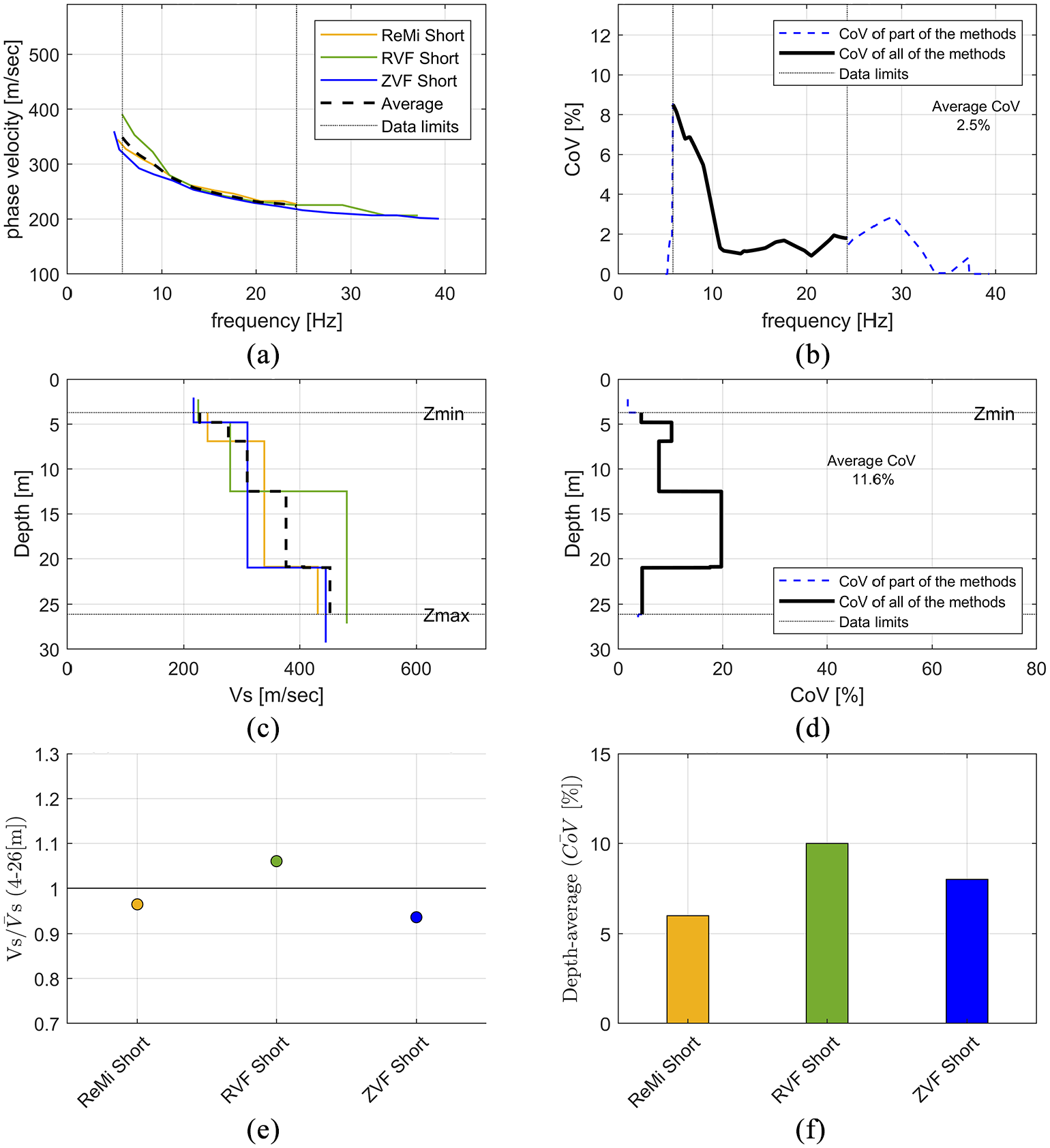
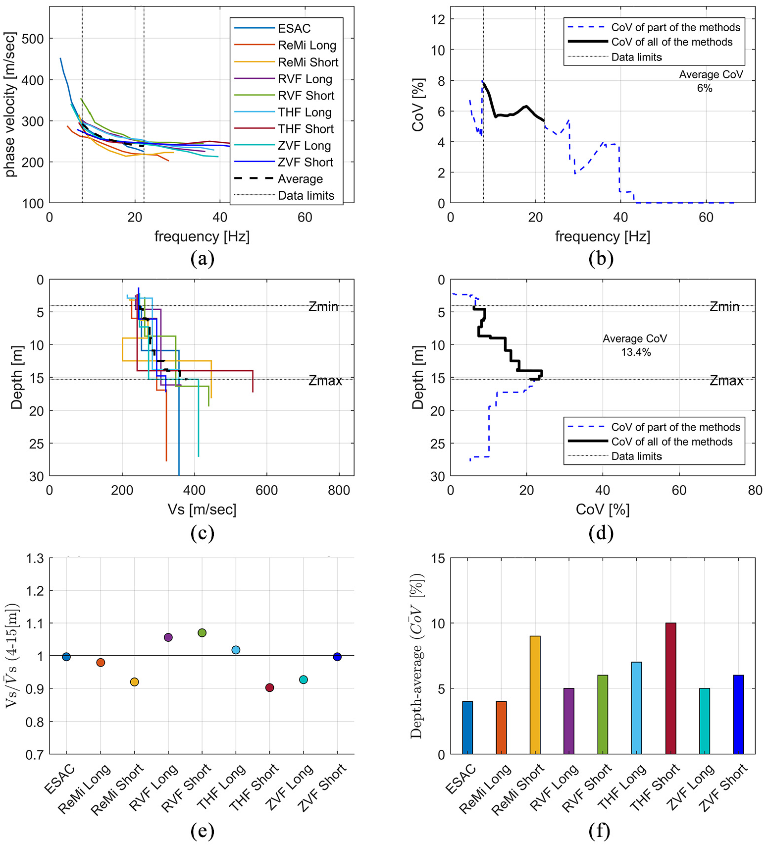
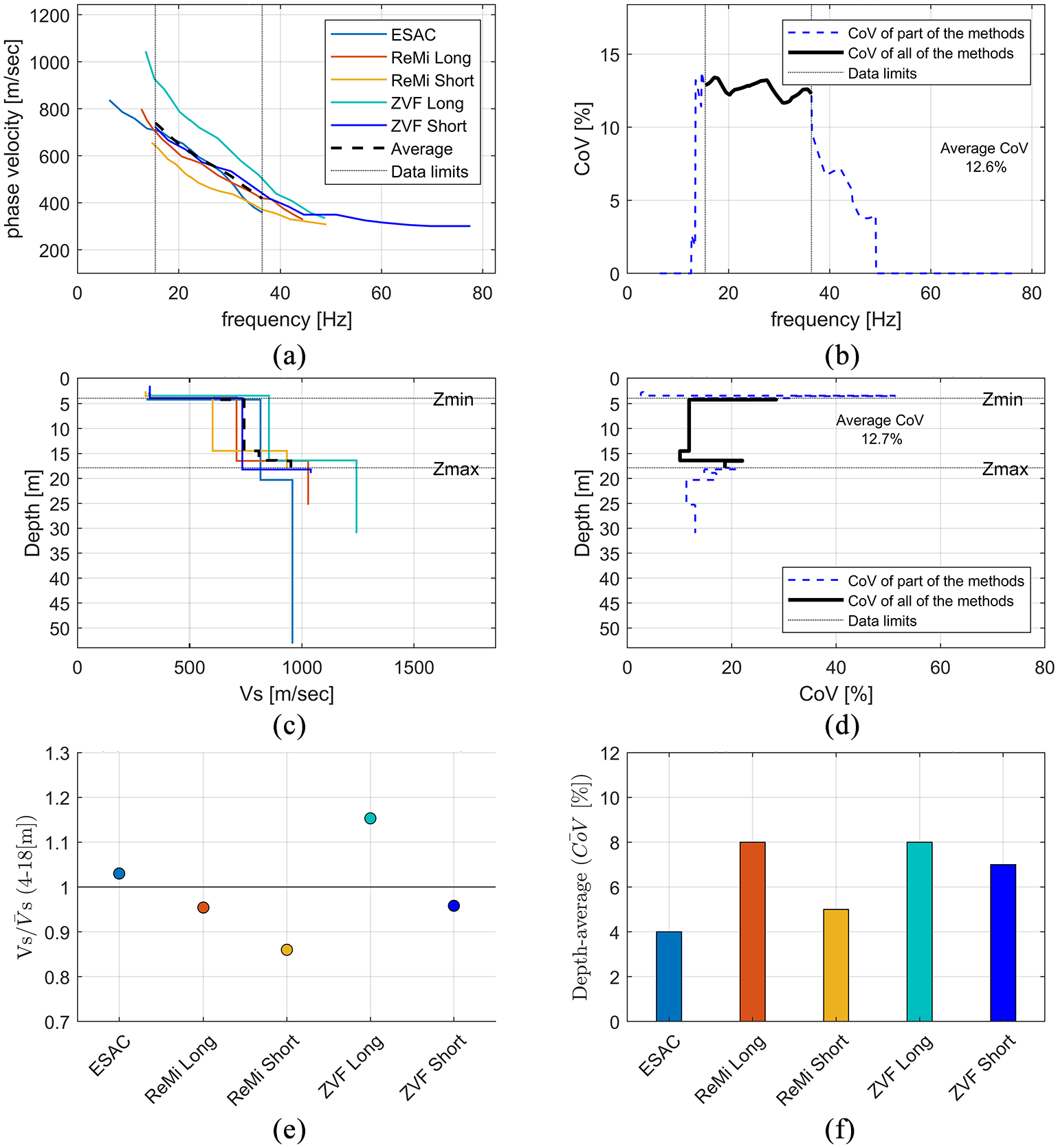
Figures 6 to 11 display the results for each site, where each figure is divided into six sections: (a) the family of dispersion curves picked from each of the different methods, the average dispersion curve, and the frequency boundaries for inter-method comparison (between methods). (b) The inter-method variability of the theoretical dispersion curves. The variability of the results is evaluated through a coefficient of variation (CoV) which defined as:

CoV = (σ / μ) \cdot 100 %

(1)

where $σ$ is the standard deviation and $μ$ is the mean value of the population of results. (c) and (d) are the same as (a) and (b) but refer to the shear-wave profiles instead of their dispersion curves. For both (b) and (d) panels, the black curves represent the CoV, which is calculated from all of the methods, while the blue dot curve is the CoV of part of the methods. (e) The normalized inter-method variability is defined as:

\frac{{V_{S}}_{z (\max)}^{z (\min)}}{{\bar{V}}_{S}_{z (\max)}^{z (\min)}}

(2)

Figure 6.

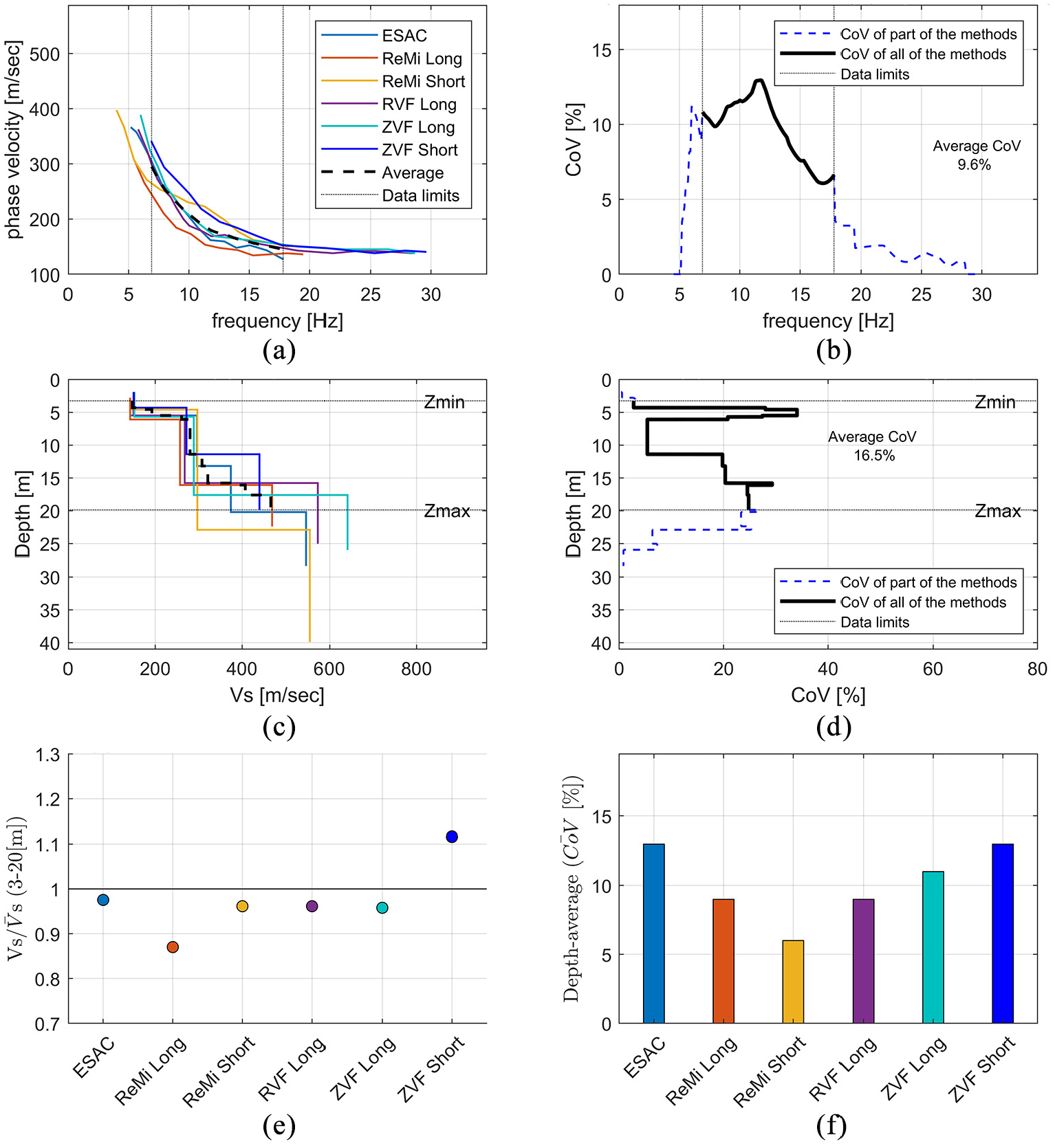
The BET site results (see text for more information): (a) dispersion curves, (b) inter-method variability (dispersion curves), (c) Vs profiles, (d) inter-method variability (Vs), (e) normalized inter-method variability, and (f) intra-method variability.

Figure 7.

The BSH site results (see text for more information): (a) dispersion curves, (b) inter-method variability (dispersion curves), (c) Vs profiles, (d) inter-method variability (Vs), (e) normalized inter-method variability, and (f) intra-method variability.

Figure 8.

The CAS site results (see text for more information): (a) dispersion curves, (b) inter-method variability (dispersion curves), (c) Vs profiles, (d) inter-method variability (Vs), (e) normalized inter-method variability, and (f) intra-method variability.

Figure 9.

The HOD site results (see text for more information): (a) dispersion curves, (b) inter-method variability (dispersion curves), (c) Vs profiles, (d) inter-method variability (Vs), (e) normalized inter-method variability, and (f) intra-method variability.

Figure 10.

The MGH site results (see text for more information): (a) dispersion curves, (b) inter-method variability (dispersion curves), (c) Vs profiles, (d) inter-method variability (Vs), (e) normalized inter-method variability, and (f) intra-method variability.

Figure 11.

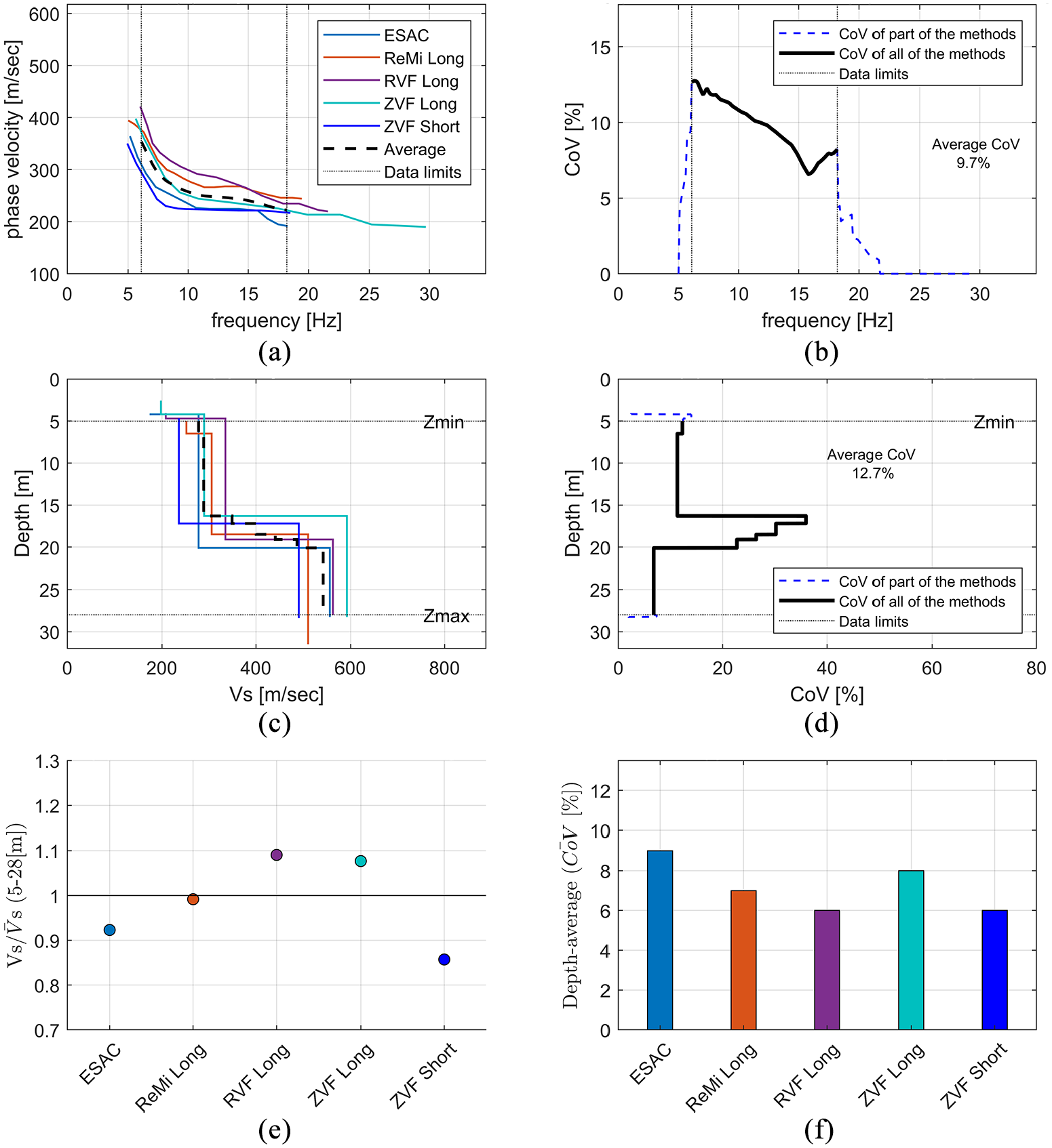
The RAM site results (see text for more information): (a) dispersion curves, (b) inter-method variability (dispersion curves), (c) Vs profiles, (d) inter-method variability (Vs), (e) normalized inter-method variability, and (f) intra-method variability.

The numerator is the time-averaged shear wave velocity for the investigation depth range. The denominator ${\bar{V}}_{S}_{z (\max)}^{z (\min)}$ is the average value of all ${V_{S}}_{z (\max)}^{z (\min)}$ measured at a specific site. The time-averaged shear wave velocity is calculated according to:

{V_{S}}_{z (\max)}^{z (\min)} = \frac{z (\max - \min)}{\sum_{i = z (min)}^{z (max)} \frac{H_{i}}{V_{s, i}}}

(3)

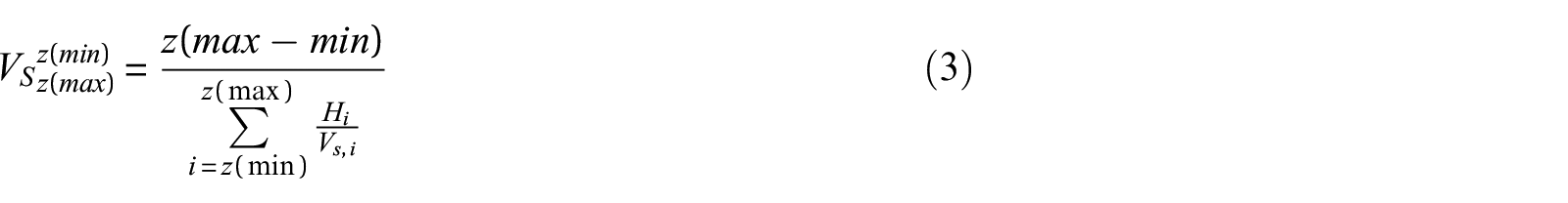
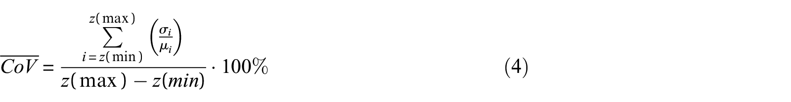
where H_i is the thickness and V_S,i is the shear wave velocity for each layer i. The maximum investigated depth, z(max), is assumed to be roughly between a third to a half of the maximum observed wavelength (Dal Moro, 2014; Foti et al., 2014). Hence, I limited the maximum investigated depth to be approximately 40% of the maximum retrieved wavelength. For shallow depths, z(min) is defined as 40% of the minimum retrieved wavelength. The V_S profile will never start at the surface, thus avoiding the part of the section that is under-sampled. (f) The intra-method variability (the variability within the method) for each method is defined as the depth-average of the CoV from the minimum to the maximum investigation depth, z(min) to z(max), respectively. It represents the uncertainties of the inversion process and defined as:

\bar{CoV} = \frac{\sum_{i = z (min)}^{z (max)} (\frac{σ_{i}}{μ_{i}})}{z (max) - z (\min)} \cdot 100 %

(4)

where $σ$ is the standard deviation and $μ$ is the mean value of the population of results.

Table 2 summarizes the results of the six sites. The table lists the number of tests, range of depths for which all measurements are available, maximum CoV, $\bar{CoV}$ , maximum normalized $({V_{S}}_{z (\max)}^{z (\min)})$ , and the intra-method variability.

Table 2.

Summary of the results

Site	# of tests	Zmin toZmax (m)	V_S Inter-method variability (%)			Dispersion curveinter-method variability (%)		Intra-methodvariability, $\bar{CoV}$ (%)
			MaximumCoV (%)	AverageCoV (%)	MaximumnormalizeV_S,Z(max-min)	MaximumCoV (%)	AverageCoV (%)
BET	6	3–20	35	16.5	0.88	12.5	9.6	6–13
BSH	5	6–27	35	16.1	0.92	13	5.2	4–14
CAS	3	4–26	20	11.6	1.06	8.3	2.5	6–10
HOD	9	4–15	25	13.4	0.9	8.0	6.0	4–10
MGH	5	4–18	28	12.7	1.15	13.5	12.6	4–8
RAM	5	5–28	35	12.7	0.86	12.5	9.7	6–9

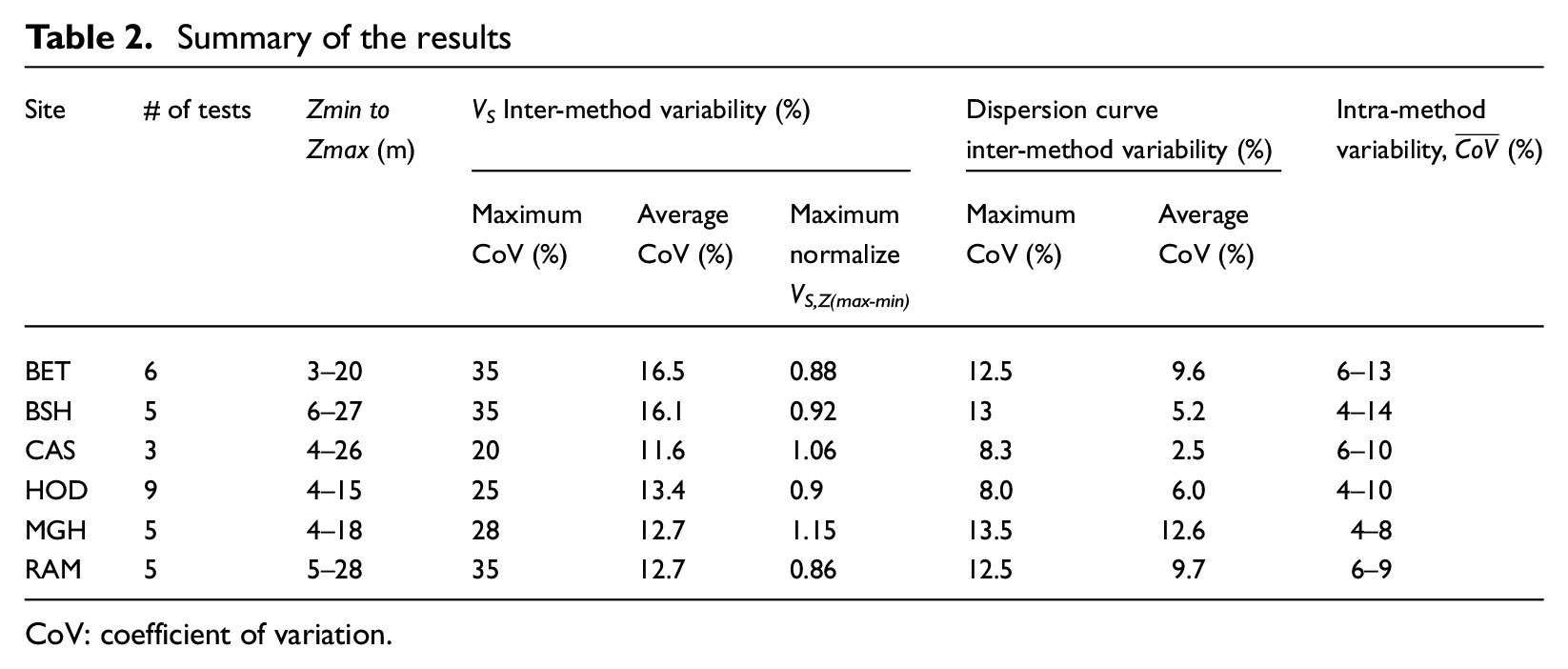
CoV: coefficient of variation.

Figure 12 displays the noise analysis of each site: the HVSR overtime in which each curve is calculated over a time window sample of 20–30 s. HVSR directivity shows the azimuth of the signals, and the amplitude spectra illustrate the spectrum of the site.

Figure 12.

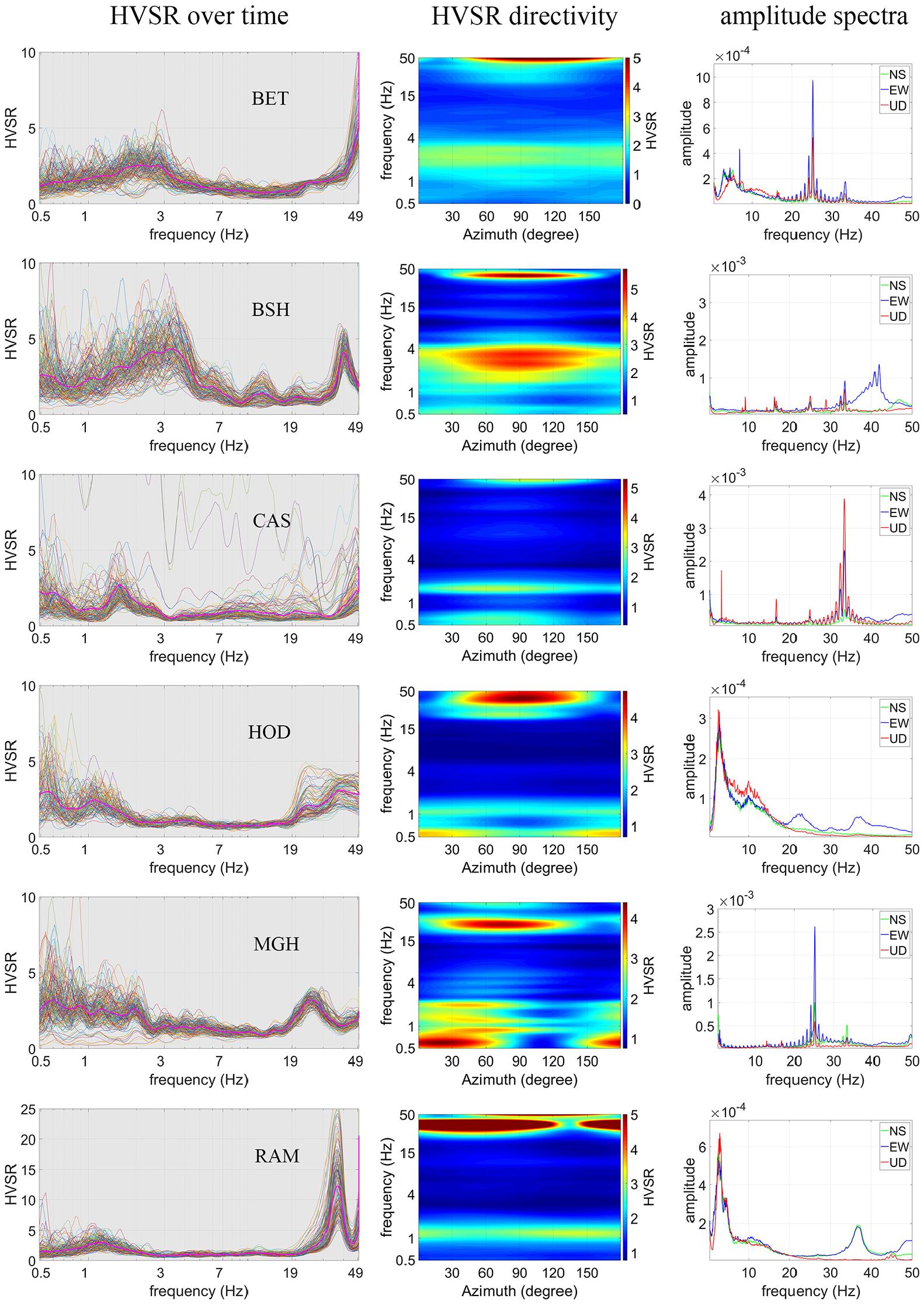
Background “Noise” analysis. Each row represents a site. The first column is the HVSR over time, in which each curve is a sample representing a window of 20–30 s. The second column is the HVSR directivity, and the third column is the amplitude spectra.

It is worth mentioning that RVF refers to the vertical component (SV) of the shear wave and THF refers to the horizontal component (SH). Hence, anisotropy may explain some of the small variations between the two components which were integrated together in the analysis, that is, no separation between SH and SV.

Discussion

Our results indicate well-defined uncertainties in the measurements at the six different industry sites. The discussion below focuses on what is expected and measured in industrial sites in terms of the induced bias from the noise wavefield. I will also focus on the inter-method and intra-method comparisons and the depth of penetration for the various methods.

Misinterpretation in the identification of the dispersion curve modes (fundamental mode vs higher modes) can bias the results and is not covered in this study. In addition, the inversion process attempts to converge the solution to the local minimum. Thus, the introduction of known information (e.g. stratigraphic logs and water table depth) can constrain the inversion results and would certainly reduce the variability of the V_S profile. Known information was not available in this study.

The influence of the industrial seismic noise

Seismic noise in cities, and particularly in industrial areas, is driven by numerous processes such as transportation, machinery, humans, and so on. It is expected that these areas will be characterized by an unnatural wavefield, which may include sharp spikes within the amplitude spectra, amplitude variation within the spectrograms, and also a preferential direction of the HVSR measurement. Unsurprisingly, these phenomena are viewed in our observations (Figure 12).

The HVSR curves over time (Figure 12) indicate a significant variation between the samples at each site. For example, in the BSH site at ∼12 Hz, the HVSR varies for different sampling windows from 0.5 to 3.5, while from 1 to 4 Hz, it also varies significantly from 0.5 to 9. Also, in most of the sites, the HVSR directivity represents a preferential direction of the signal. For example, the HVSR directivity at the MGH site indicates seismic signals from different directions and frequencies; 2 Hz in azimuth between 30 and 60 degrees and ∼27 Hz in an azimuth mainly between 60 and 90 degrees. The amplitude spectra of all six sites are characterized by several sharp spikes that are probably due to noisy local machines.

This observation of HVSR over time, HVSR directivity, and amplitude spectra (also spectrograms within the Supplementary) indicate that some of the frequencies are biased due to industrial sources. However, a closer look at the biased frequencies at the HVSR over time and HVSR directivity reveal that most of the sites have biased frequencies lower than 4 Hz or higher than 20 Hz. The meaning of this is that they are beyond the uncertainty comparisons. Besides, despite the sharp spikes which influence most of the spectra at most of the sites, the data quality and especially the dispersion images are not compromised, even if the industrial noised is not eliminated (Figure 13).

Figure 13.

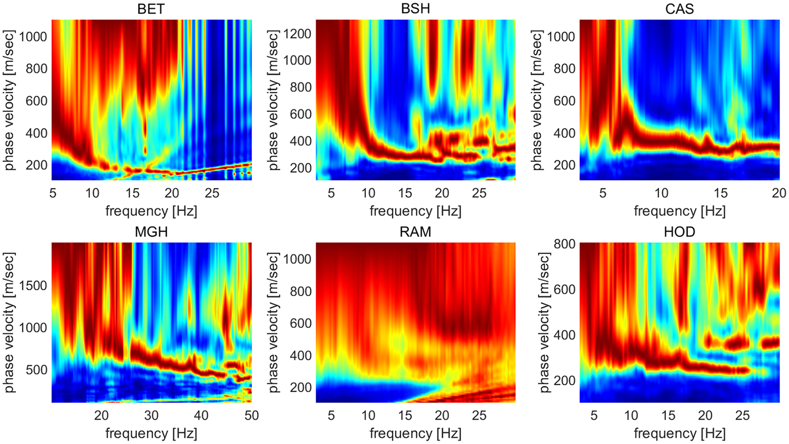
The ReMi dispersion images of all six sites.

Inter-method variability

The agreement between the experimental dispersion curves at each site is very satisfactory, with an average CoV that varies from 2.5% to 12.6% (panel b in Figures 6 to 11 and Table 2). This confirms the robustness of the estimate of the experimental dispersion curve by the different methods, an observation consistent with previous studies (Cornou et al., 2006; Cox et al., 2014). CoVs for the dispersion relations are lower than CoVs for the V_S profiles, where the last shows higher variability. The maximum CoV of the V_S profiles varies from 20% to 35% (Table 2). These relatively high CoV values are an outcome of the thickness uncertainties for each layer. For instance, at the RAM site, the CoV values of the V_S profile are about 26%–35% at depths from ∼16 to ∼20 m (Figure 11d). More specifically, for a thickness of less than a meter, at depths of ∼16 to ∼17 m, the CoV value is about 35%. This strong contrast is seen in most of our results and is due to the thickness uncertainties and might be less if common layering was used for the comparison.

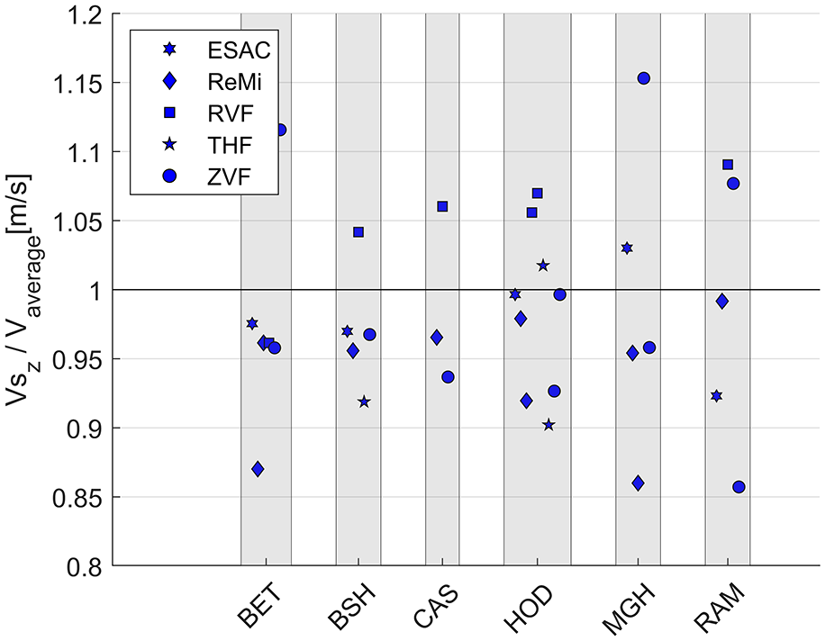
Compared to the maximum CoV values, those of the average shear-wave profiles $({\bar{V}}_{S}_{z (\max)}^{z (\min)})$ for all methods are no more than 16.5% (Table 2). Also, the maximum normalized values (Equation 1) vary between ∼0.85 and ∼1.15 at the MGH site (Figure 14). These results are slightly lower than another comparison analysis measured in Israel (Kamai et al., 2018). The variation of the normalized inter-method variability is low compared to the depth-dependent CoV. Therefore, the influence of anomalies within each V_S profile is lower. This indicates the robustness of the surface-wave methods for the computation of V_S,Z and for the global parameter, V_S,30.

Figure 14.

Inter-method variability—the normalized V_{S, Z} of each method at all sites.

It is expected that the CoV values would increase with depth due to lower resolution in deeper layers. However, since in all our sites, the V_S profile increases with depth, the CoV values should be smaller at depth (due to the linear calculation of CoV). In any case, in our six sites, there is no correlation between the CoV values and depth (Figures 6 to 11, panel d).

Intra-method variability

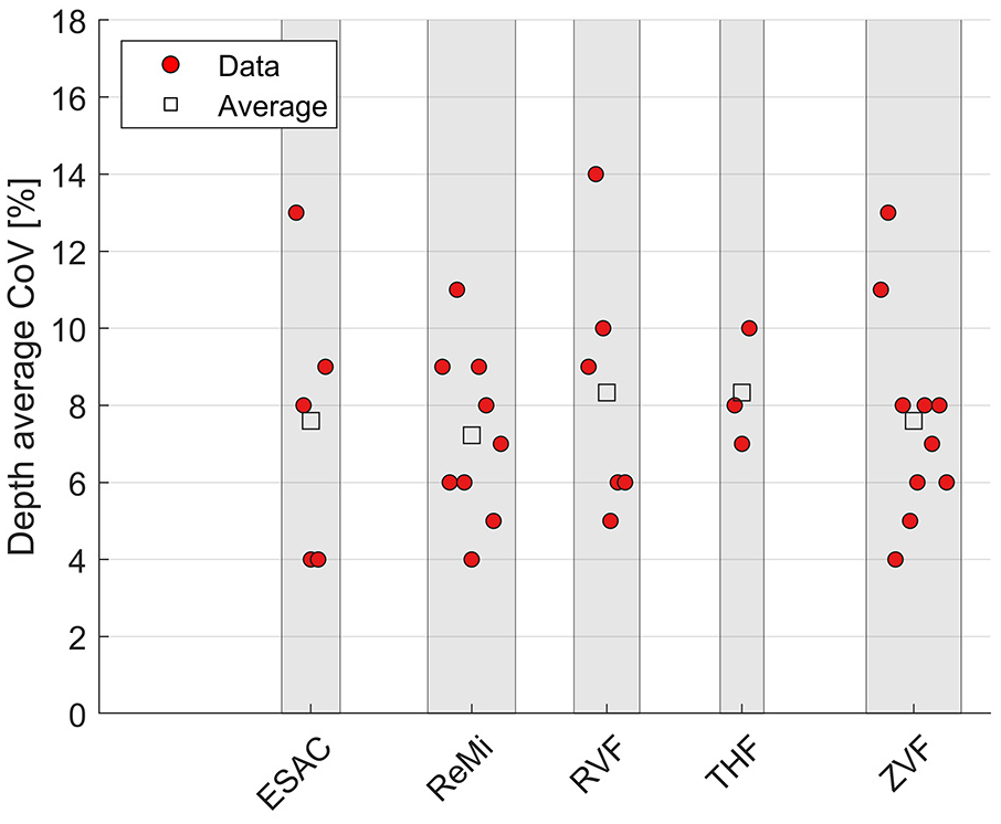
The calculated $\bar{CoV}$ for each method at each site varies from 4% to a maximum of 14%, with average values from 7.7% to 9.8% for the six different methods (Figure 15). This intra-method variability is relatively low in comparison to the inter-method variability and probably is insignificant in geotechnical engineering and GMPE terms. The cloud of scatter points (Figure 15) indicates that there is no correlation between the method and the CoV. The average black rectangles highlight this finding.

Figure 15.

Intra-method variability—the $\bar{CoV}$ of each method at all six sites which reflect only the inversion processing stage.

The low CoV values within the intra-method variability reflect only the inversion processing stage. This is because I compare data from the same deployments for each site. I also use the same sources for active methods, and I did not process the data differently. Hence, the inversion processing stage is the only stage presenting variation. The surface wave inverse problem is mathematically ill-posed, and it is affected by solution non-uniqueness (Luke et al., 2003). Therefore, several different shear-wave profiles can produce the same theoretical dispersion curve.

Depth of investigation

Besides the instrumental limits (sensor and source), two main factors will define the depth of investigation: the V_S structure and the lower frequencies that will be picked over the dispersion image. As the velocities are lower, the depth of investigation will probably be shallower. According to a practical rule of thumb, the maximum depth of investigation is a half to a third of the longest picked wavelength (velocity divided by the frequency). For example, a maximum of about 13–20 m depth of investigation applies to a site in which the velocity is 200 (m/s) at 5 Hz (the lower picked frequency). For comparison, if the velocity is 1000 (m/s) at the same frequency, the maximum depth of investigation is five times larger, 67–100 m. Usually, active methods provide higher frequencies than passive methods. Therefore, they are more suitable for the characterization of the very shallow layer, in comparison to passive techniques, which are better for deep characterization. This is primarily because the passive signals are of generally lower frequency than active sources (Garofalo et al., 2016a). Accordingly, I assume that deeper data will be available from passive rather than active measurements. Indeed, in our study, there is a correlation between the method and the maximum depth of investigation (Figure 16); the passive tests, particularly the ESAC method, provide information from a deeper range than the active ones.

Figure 16.

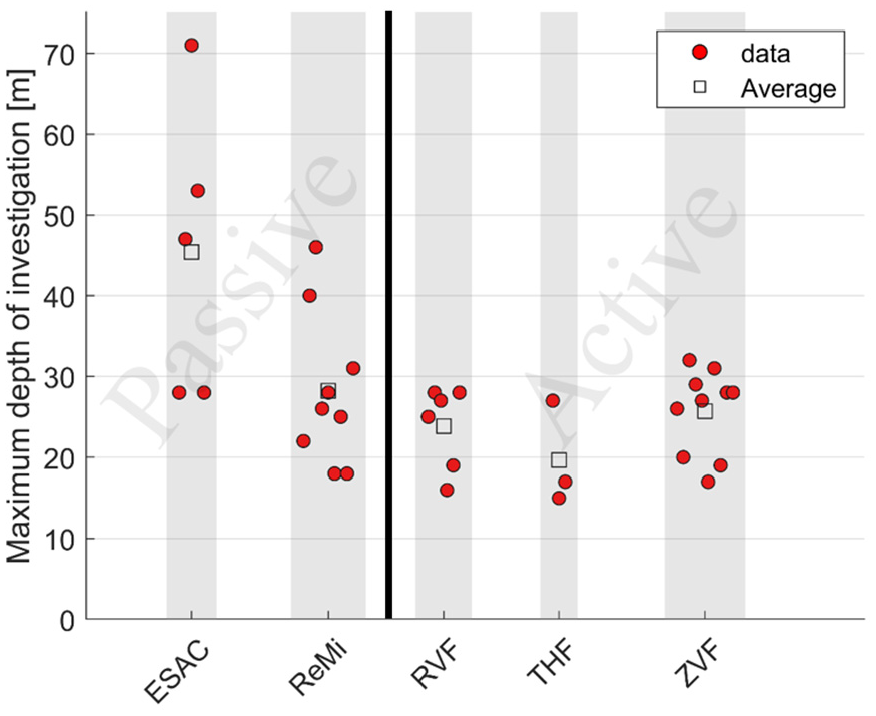
Maximum depth of investigation following the different methods.

Certainly, to provide a better constraint to the model, both in the shallow and the deep subsurface, a combination of the information from both active and passive data is essential (Garofalo et al., 2016b). However, this discussion is beyond the scope of this study.

Conclusion

In this study, I explored six different sites located in noisy environments. I acquired data by five different types of surface-wave methods and compared the results to estimate the inter-method and intra-method variabilities at each site. The purpose of the research was to apply common practice site characterization approaches while also evaluating approaches not commonly applied (RVF, THF). Our results indicate that, while the average CoV of the different dispersion curves is up to ∼13% at specific frequencies, the frequency-averaged CoV is about 8%. The same concept holds for the CoV of the V_S profile, which peaks at 35% for specific depths. However, for the various sites, the depth-averaged CoV ranges from ∼12% to ∼17%. This indicates that the uncertainty of the individual methods can lead to significant misinterpretation of the shallow subsurface.

On the contrary, the average index V_S,Z is less sensitive to these uncertainties and is therefore much more robust. This reaffirms its use (mainly V_S,30) in building codes and within GMPE. The uncertainty for each test, of the 33 acquired, varies from 4% up to 14%, and there is no correlation between the test type and the CoV. These findings imply that while there is no preferred method, it is still advisable to use several methods to collect data.

In our tests, the data available for deeper depths came from the passive tests, particularly from the ESAC method. These confirm the common wisdom that passive tests provide lower frequencies than active methods and therefore are more suitable for deeper seismic characterization.

It is possible that more robust survey design using best practices may result in much lower uncertainty. These may include longer arrays, larger energy sources for active source data acquisition, and use of passive arrays with better azimuthal averaging (T shape, fan shape, triangular, circular, etc.).

Although our study focuses on surface-wave measurements in noisy environments, it aligns with comparable shear-wave studies and falls within the acceptable uncertainties in the results. This suggests that such tests are also applicable in industrial zones where the signals processed may be affected by noise. This conclusion has practical implications for use in estimating seismic hazards in industrial zones.

Supplemental Material

sj-docx-1-eqs-10.1177_8755293020988029 – Supplemental material for Shear-wave velocity measurements and their uncertainties at six industrial sites

Supplemental material, sj-docx-1-eqs-10.1177_8755293020988029 for Shear-wave velocity measurements and their uncertainties at six industrial sites by Yaniv Darvasi in Earthquake Spectra

Footnotes

Acknowledgements

I thank HUJI’s Neev Center for Geoinfomatics for its equipment and computational facilities and the great contribution of labor and assistance from its students. I am especially grateful to Dr John K. Hall and Prof. Amotz Agnon, co-founders of the Center. I thank Amos Shiran and Hanan Alexander for advice and support. Finally, I especially thank Eli Ram for his field assistance.

Declaration of conflicting interests

The author(s) declared no potential conflicts of interest with respect to the research, authorship, and/or publication of this article.

Funding

The author(s) received no financial support for the research, authorship, and/or publication of this article.

ORCID iD

Yaniv Darvasi

Supplemental material

Supplemental material for this article is available online.

References

Abrahamson

Silva

(2008) Summary of the Abrahamson & Silva NGA ground-motion relations. Earthquake Spectra 24(1): 67–97.

Arai

Tokimatsu

(2004) S-wave velocity profiling by inversion of microtremor H/V spectrum. Bulletin of the Seismological Society of America 94(1): 53–63.

Bard

(1998) Microtremor measurement: A tool for site effect estimation? In: Irikura

Kudo

Okada

Sasatami

(eds) The Effects of Surface Geology on Seismic Motion. Balkema: Rotterdam, pp. 1251–1279.

Bard

Acerra

Alguacil

Anastasiadis

Atakan

Azzara

, et al. (2004) Guidelines for the implementation of the H/V spectral ratio technique on ambient vibrations measurements, processing and interpretation. Interpretation A Journal of Bible and Theology 169: 1–62.

Bazzurro

Cornell

(2004) Nonlinear soil-site effects in probabilistic seismic-hazard analysis. Bulletin of the Seismological Society of America 94(6): 2110–2123.

Boore

(2006) Determining subsurface shear-wave velocities: A review. In: Third international symposium on the effects of surface geology on seismic motion (eds Bard

P.-Y

Chaljub

Conrou

Cotton

Gueguen

), Grenoble, France, 30 August–1 September, pp. 1–21. Paris: Laboratoire Central des Ponts et Chauss\’ees.

Boore

Asten

(2008) Comparisons of shear-wave slowness in the Santa Clara Valley, California using blind interpretations of data from invasive and noninvasive methods. Bulletin of the Seismological Society of America 98(4): 1983–2003.

Building Seismic Safety Council (1997) NEHRP (National Earthquake Hazards Reduction Program) recommended provisions for seismic regulations for new buildings and other structures. FEMA 302: 303.

European Committee for Standardization (CEN) (2004) Design of structures for earthquake resistance. Eurocode 8: Part 1: General Rules, Seismic Actions and Rules for Buildings, European Standard EN 1998-1. Brussels.

10.

Cornou

Ohrnberger

Boore

, et al. (2006) Derivation of structural models from ambient vibration array recordings: Results from an international blind test. In: Third international symposium on the effects of surface geology on seismic motion, Grenoble, France, 30 August–1 September, pp. 1127–1219. Paris: Laboratoire Central des Ponts et Chauss\’ees.

11.

Cox

Wood

Teague

(2014) Synthesis of the UTexas1 surface wave dataset blind-analysis study: Inter-analyst dispersion and shear wave velocity uncertainty. In: Proceedings of geo-congress 2014 (ed Yu

), Atlanta, Georgia, 23-26 February 2014, pp.850859. Reston: American Society of Civil Engineers.

12.

Dal Moro

(2014) Surface Wave Analysis for Near Surface Applications. Amsterdam, The Netherlands: Elsevier.

13.

Dal Moro

Pipan

Gabrielli

(2007) Rayleigh wave dispersion curve inversion via genetic algorithms and Marginal Posterior Probability Density estimation. Journal of Applied Geophysics 61(1): 39–55.

14.

Foti

(2000) Multistation methods for geotechnical characterization using surface waves. Politecnico di Torino PhD Dissertation 42: 315–323.

15.

Foti

Lai

Rix

, et al. (2014) Surface Wave Methods for Near-Surface Site Characterization. Boca Raton, FL: CRC Press.

16.

Garofalo

Foti

Hollender

, et al. (2016a) InterPACIFIC project: Comparison of invasive and non-invasive methods for seismic site characterization. Part II: Inter-comparison between surface-wave and borehole methods. Soil Dynamics and Earthquake Engineering 82: 241–254.

17.

Garofalo

Foti

Hollender

, et al. (2016b) InterPACIFIC project: Comparison of invasive and non-invasive methods for seismic site characterization. Part I: Intra-comparison of surface wave methods. Soil Dynamics and Earthquake Engineering 82: 222–240.

18.

Gucunski

Woods

(1991) Instrumentation for SASW testing. In: Bhatia

Blaney

(eds) Recent Advances in Instrumentation, Data Acquisition and Testing in Soil Dynamics, Orlando: American Society of Civil Engineers. pp.1–16.

19.

Haines

(2007) A hammer-impact, aluminium, shear-wave seismic source. Open-File Report 2007–1406. Reston, VA: U.S. Geological Survey.

20.

Hamiel

Masson

Piatibratova

, et al. (2018) GPS measurements of crustal deformation across the southern Arava Valley section of the Dead Sea Fault and implications to regional seismic hazard assessment. Tectonophysics 724–725: 171–178.

21.

Hatzor

(2000) Geological Map of Israel 1: 50,000, Bet She’an. Jerusalem, Israel: Geological Survey of Israel.

22.

Hofstetter

Van Eck

Shapira

(1996) Seismic activity along fault branches of the Dead Sea-Jordan transform system: The Carmel-Tirtza fault system. Tectonophysics 267(1–4): 317–330.

23.

Horike

(1996) Geophysical exploration using microtremor measurements. In: Proceedings of the 11th world conference on earthquake engineering by International Association for Earthquake Engineering, Acapulco, Mexico, 23–28 June 1996.

24.

Kagan

Stein

Agnon

, et al. (2011) Intrabasin Paleoearthquake and quiescence correlation of the late Holocene Dead Sea. Journal of Geophysical Research: Solid Earth 116(B4): B04311.

25.

Kamai

Abrahamson

Silva

(2016) VS30 in the NGA GMPEs: Regional differences and suggested practice. Earthquake Spectra 32(4): 2083–2108.

26.

Kamai

Darvasi

Peleg

, et al. (2018) Measurement and interpretation uncertainty in site response of nine seismic network stations in Israel. Seismological Research Letters 89(5): 1796–1806.

27.

Louie

(2001) Faster, better: Shear-wave velocity to 100 meters depth from refraction microtremor arrays. Bulletin of the Seismological Society of America 91(2): 347–364.

28.

Luke

Calderón-Macías

Stone

, et al. (2003) Non-uniqueness in inversion of seismic surface-wave data. In: Proceedings of the 16th EEGS symposium on the application of geophysics to engineering and environmental problems: Environmental and Engineering Geophysical Society, Denver, USA, 6 April 2003, pp.1342-1347. SEG: Environment and Engineering Geophysical Society Environment and Engineering Geophysical Society.

29.

Moss

RES

(2008) Quantifying measurement uncertainty of thirty-meter shear-wave velocity. Bulletin of the Seismological Society of America 98(3): 1399–1411.

30.

Mucciarelli

Gallipoli

(2001) A critical review of 10 years of microtremor HVSR technique. Bollettino di Geofisica Teorica ed Applicata 42(3–4): 255–266.

31.

Nolet

(1981) Linearized inversion of (teleseismic) data. In: Cassinis

(ed.) The Solution of the Inverse Problem in Geophysical Interpretation. Boston, MA: Springer, pp. 9–37.

32.

Ohori

Nobata

Wakamatsu

(2002) A comparison of ESAC and FK methods of estimating phase velocity using arbitrarily shaped microtremor arrays. Bulletin of the Seismological Society of America 92(6): 2323–2332.

33.

Park

Miller

Xia

(1998) Imaging dispersion curves of surface waves on multi-channel record. In: 68th annual international SEG, New Orleans, 13–18 September 1998, pp.1377-1380. Technical Program Expanded Abstracts.

34.

Park

Miller

Xia

(1999) Multichannel analysis of surface waves. Geophysics 64(3): 800–808.

35.

Rathje

Kottke

Trent

(2010) Influence of input motion and site property variabilities on seismic site response analysis. Journal of Geotechnical and Geoenvironmental Engineering 136(4): 607–619.

36.

Sharon

Sagy

Kurzon

, et al. (2020) Assessment of seismic sources and capable faults through hierarchic tectonic criteria: Implications for seismic hazard in the Levant. Natural Hazards and Earth System Sciences 20(1): 125–148.

37.

Sneh

Rosensaft

(2004) Geological Map of Israel 1: 50,000, Rishon LeZion. Jerusalem, Israel: Geological Survey of Israel.

38.

Sneh

Rosensaft

(2008) Geological Map of Israel 1: 50,000, Tel Aviv. Jerusalem, Israel: Geological Survey of Israel.

39.

Socco

Strobbia

(2004) Surface-wave method for near-surface characterization: A tutorial. Near Surface Geophysics 2(4): 165–185.

40.

Stokoe

Wright

Bay

, et al. (1994) Characterization of geotechnical sites by SASW method. In: Woods

(ed) Geophysical Characterization of Sites. New Delhi: Oxford & IBH Publishers, pp.15–25.

41.

Xia

Miller

Park

, et al. (2002) Comparing shear-wave velocity profiles inverted from multichannel surface wave with borehole measurements. Soil Dynamics and Earthquake Engineering 22(3): 181–190.

Supplementary Material

Please find the following supplemental material available below.

For Open Access articles published under a Creative Commons License, all supplemental material carries the same license as the article it is associated with.

For non-Open Access articles published, all supplemental material carries a non-exclusive license, and permission requests for re-use of supplemental material or any part of supplemental material shall be sent directly to the copyright owner as specified in the copyright notice associated with the article.

0.00 MB

28.85 MB