Sage Journals: Discover world-class research

Abstract

The need for US Geological Survey (USGS) National Seismic Hazard Models (NSHMs) to report estimates of epistemic uncertainties in the hazard (e.g. fractile hazard curves) in all forthcoming releases is increasing. With fractile hazard curves as potential new outputs from the USGS 2023 NSHM, a simultaneous need is to help end-users better understand these epistemic uncertainties and clarify their potential uses. In this article, we address the latter need by (1) characterizing epistemic uncertainties in two updates of the USGS NSHM (2014 for California and 2021 for Hawaii), (2) illustrating a variety of downstream applications of fractile hazard curves in both hazard and risk contexts, and (3) discussing implications from the various types of uncertainties. We found that the epistemic uncertainty in hazard is generally larger for Hawaii than for California, the epistemic uncertainty in hazard can be reasonably approximated with a lognormal distribution for most of the cases considered, and the correlation between epistemic uncertainty in hazard at two different intensity measure levels generally varies with both location and type of intensity measure. Furthermore, we developed models for readily generating approximate fractile hazard curves in California and Hawaii. Finally, given the complexities involved in the hazard modeling process, we developed an open-source interactive tool to enable a broad range of users to independently examine and potentially start using such epistemic uncertainties for their respective applications.

Keywords

USGS 2023 National Seismic Hazard Model fractile epistemic uncertainty

Introduction

The US Geological Survey (USGS) National Seismic Hazard Models (NSHMs) have traditionally reported mean hazard curves but not “fractile” hazard curves¹ (Petersen et al., 2008, 2015, 2020). In essence, a single hazard curve at a given location quantifies the “aleatory variability” in ground shaking, whereas different hazard curves at the same location represent the “epistemic uncertainty” in the hazard (Abrahamson and Bommer, 2005; Ang and Tang, 2007; Musson, 2012). While the distinction between the two terms is not always obvious, the distinction is still useful in some contexts² (Der Kiureghian and Ditlevsen, 2009; McGuire et al., 2005). Epistemic uncertainty exists in the hazard because of limited data and knowledge in defining the (1) seismic source model (SSM) and (2) ground motion model (GMM) (Anderson, 2018; Budnitz et al., 1997; Cao et al., 2005; Cramer, 2001; McGuire, 1977; National Research Council (NRC), 1988). For example, several alternative models might be available to characterize earthquake occurrences in time, spatial geometry of earthquake sources, and exceedances of ground motion levels for different earthquake ruptures (Bradley, 2009; Working Group on California Earthquake Probabilities, 2003). One way to capture such alternatives and their scientific credibility is through explicit documentation using logic trees (Baker et al., 2021; Bommer et al., 2005; Kulkarni et al., 1984; McGuire, 2004).

As the USGS continues to update the NSHM, the need to report estimates of epistemic uncertainties in the hazard is increasing (e.g. National Academies of Sciences, Engineering, and Medicine (NASEM), 2019; NSHM Steering Committee, 2020). For example, “more complete calculation of uncertainties (fractiles) in the hazard models” was planned at the conclusion of the 2018 update (Petersen et al., 2020). For the first time, fractile-based uniform hazard ground motions (UHGMs) were recently reported for the 2021 update of the NSHM for Hawaii (Petersen et al., 2022). Reporting estimates of epistemic uncertainties in the hazard is important because a probabilistic seismic hazard analysis should (1) “account for uncertainties in a complete and transparent way,” and (2) “adopt decision methods that are insensitive to alternative valid interpretations” (McGuire et al., 2005).

At the same time, helping end-users of the NSHM better understand such epistemic uncertainties and their uses is important. For example, although logic trees have traditionally been already used to capture epistemic uncertainties when deriving mean hazard, past NSHMs have reported only the mean hazard (Altekruse and Powers, 2021; Frankel et al., 1996, 2002; Shumway et al., 2021). Consequently, misinterpretation and confusion are possible if epistemic uncertainties in the hazard were also to be reported in every forthcoming update (e.g. via fractile hazard curves at select locations), especially because the end-users of the NSHM are wide ranging (e.g. design engineers, risk modelers, and researchers). Moreover, how epistemic uncertainties in the hazard are used is highly context-specific (e.g. Hamburger et al., 2017; Lee et al., 2018).

Therefore, this article aims to help end-users of the NSHM better understand epistemic uncertainties in the hazard and their potential uses. To achieve this goal, this article focuses on various downstream applications of the epistemic uncertainties in hazard after they have already been quantified or reported. First, we use individual logic tree branch hazard curves from two updates of the USGS NSHM (2014 for California and 2021 for Hawaii) to explicitly illustrate fractile hazard curves and clarify key ideas. Then, we characterize the nature of such epistemic uncertainties in the hazard, resulting in models for readily generating approximate fractile hazard curves in California and Hawaii. Next, we provide specific example uses of fractile hazard curves, for both hazard and risk contexts. Finally, we develop an open-source interactive tool to enable users to independently examine and potentially start using such epistemic uncertainties for their respective applications.

Epistemic uncertainties in USGS NSHMs

2014 NSHM for California

Epistemic uncertainties in the USGS 2014 NSHM for California were recently examined by researchers from the perspective of prioritizing scientific efforts (Field et al., 2020). For this goal, the study used statewide average annual loss of buildings in California to quantify the value of removing logic tree branches to reduce epistemic uncertainties in the hazard. Using a total of 172,800 logic tree branches (see Figure 3 therein), the study found that the most influential source of epistemic uncertainty was the node corresponding to “GMM Added Uncertainty” (Rezaeian et al., 2014). This node documents additional epistemic uncertainty (i.e. beyond use of multiple GMMs) to account for close interaction between developers of GMMs and lack of knowledge from earthquakes that are poorly represented in the NGA-West2 database; details for this additional epistemic uncertainty are described elsewhere (Petersen et al., 2008).

In this article, we use a subset of the full 172,800 logic tree branches to study epistemic uncertainty in hazard more comparably across two updates of the USGS NSHM. Specifically, we assume earthquake occurrences follow a Poisson probability model because USGS NSHMs provide long-term forecasts of earthquake hazard. Furthermore, we assume site effects are given by the model due to Allen and Wald (2009) because hazard curves from USGS NSHMs are reported for fixed values of time-averaged shear-wave velocity in the upper 30 m of subsurface conditions, $V_{S 30}$ . These assumptions lead to the 21,600 logic tree branches as summarized in Table 1, with each row corresponding to a logic tree node, followed by the possible branches for the given node. By choosing a branch for every row in Table 1, the resulting set of choices from all rows gives one terminal logic tree branch that corresponds to a unique hazard curve for a given type of intensity measure (e.g. 5%-damped, 1-s spectral acceleration) at a given location.

Table 1.

Logic tree used herein for illustrating fractile hazard curves in California; each row shows the branches of one node and the branch weights follow colons. Please see Figure 1 by Field et al. (2020) for definitions of abbreviations

Fault model	FM 3.1: 0.5	FM 3.2: 0.5
Deformation model	ABM: 0.1	GEOL: 0.3	NEOK: 0.3	ZENG: 0.3
Scaling relationship	EllB: 0.2	EllBsqrtLen: 0.2	HB08: 0.2	Shaw09Mod: 0.2	ShConStrDrp: 0.2
Slip along rupture	Tapered: 0.5	Uniform: 0.5
Total $M \geq 5$ rate	Rate 6.5: 0.1	Rate 7.9: 0.6	Rate 9.6: 0.3
$M_{\max}$ off fault	M7.3: 0.1	M7.6: 0.8	M7.9: 0.1
Spatial seismicity	UCERF2: 0.5	UCERF3: 0.5
GMM	ASK2014: 0.22	BSSA2014: 0.22	CB2014: 0.22	CY2014: 0.22	I2014: 0.12
GMM added uncertainty	Lower: 0.185	None: 0.63	Upper: 0.185

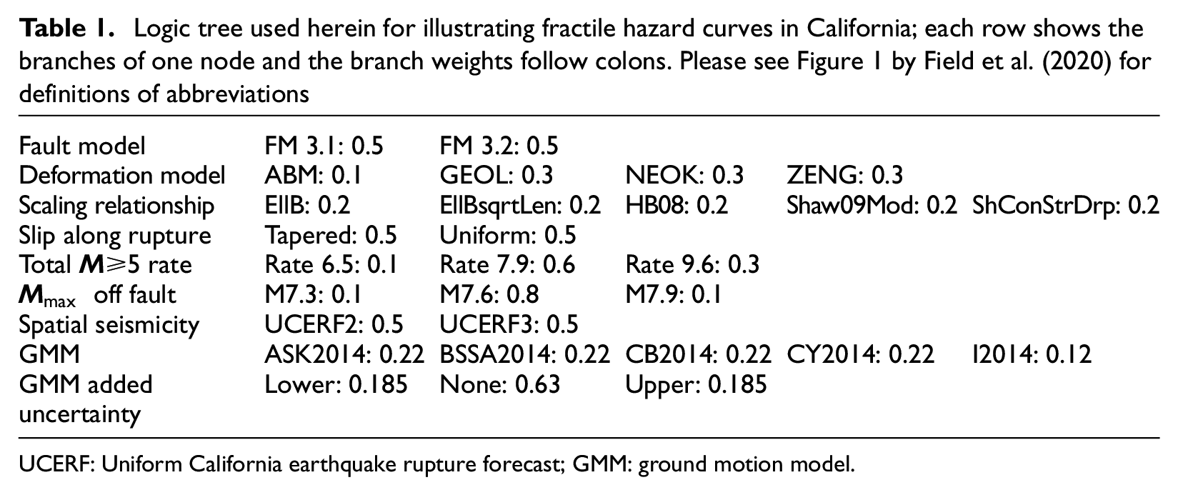
UCERF: Uniform California earthquake rupture forecast; GMM: ground motion model.

Similar to the study by Field et al. (2020), we assume the same logic tree applies to any location within California. Furthermore, we consider two types of intensity measures (0.2- and 1-s spectral accelerations, denoted respectively by SA(0.2) and SA(1.0)) and eight locations within California: (1) Los Angeles (34.1, −118.3), (2) Long Beach (33.8, −118.2), (3) Ventura (34.3, −119.3), (4) San Francisco (37.8, −122.4), (5) San Jose (37.4, −121.9), (6) Vallejo (38.1, −122.3), (7) Stockton (37.9, −121.25), and (8) Sacramento (38.52, −121.5). These intensity measure types were chosen to facilitate direct comparison with hazard from Hawaii and are important for the development of design spectra in building codes. Further, the selected locations include those considered in past USGS NSHMs (e.g. Petersen et al., 2020) as well as those considered in the study by Bradley (2009).

Unlike the study by Bradley (2009), however, we focus on annual frequencies of exceedance (AFEs) instead of 30-year probabilities of exceedance to discuss epistemic uncertainty in hazard more generally. Specifically, AFEs can be converted to probabilities using models of earthquake occurrence other than a Poisson model (e.g. Anagnos and Kiremidjian, 1988; Boyd, 2012). More precisely, we discuss AFEs in the context where earthquake occurrences and successive events are assumed to follow a homogeneous Poisson process with random selections³ (Baker et al., 2021; Der Kiureghian, 2005).

Figure 1 presents fractile hazard curves for Los Angeles and San Francisco for SA(0.2) and SA(1.0). For a given location and type of intensity measure, the shaded region illustrates the range of the individual $n_{branch} = 21, 600$ hazard curves. The mean hazard curve is shown in solid blue, which is determined from the following:

\bar{λ} (im) \equiv E [λ_{IM} (im)] = \sum_{k = 1}^{n_{branch}} w_{k} \cdot λ_{k} (im)

(1)

where im denotes a fixed level of the intensity measure, $λ_{k} (im)$ denotes the hazard curve for the $k$ th logic tree branch, $w_{k}$ denotes the corresponding logic tree branch weight, and $E [\cdot]$ denotes the mathematical expectation operator over the epistemic distribution. For a given intensity measure level, the epistemic cumulative distribution function (CDF) of AFE, $F_{λ}$ , may be determined from the following (Baker et al., 2021):

F_{λ} (l) = \sum_{k : λ_{k} \leq l} w_{k}

(2)

where $l$ denotes a fixed level of AFE, and $F_{λ}$ varies with $im$ because $λ_{k}$ varies with $im$ . Therefore, unlike the mean hazard, the $f$ th fractile hazard at a given intensity measure level, $λ_{IM, f}$ , is determined from the inverse of the epistemic CDF of AFE:

λ_{IM, f} (im) = F_{λ}^{- 1} (f)

(3)

Figure 1.

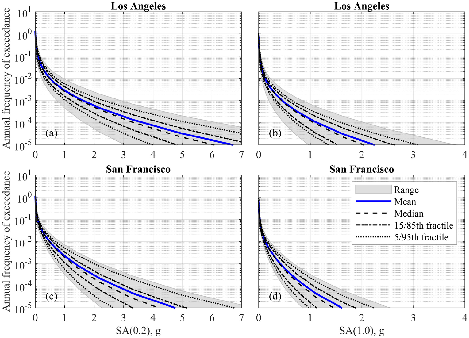
Mean and fractile hazard curves from USGS 2014 NSHM for example locations in California (21,600 branches): (a) SA(0.2) in Los Angeles, (b) SA(1.0) in Los Angeles, (c) SA(0.2) in San Francisco, and (d) SA(1.0) in San Francisco.

A few comments can be made from the results that were used to create Figure 1. First, the fractile hazard curves, which include the median hazard curve, are computed using the logic tree branch weights instead of determining quantiles from the individual 21,600 hazard curves. Therefore, none of the fractiles corresponds to a physically plausible hazard curve from a single logic tree branch.⁴ Second, the mean exceeds the median, which indicates $F_{λ}$ is positively skewed, and this difference increases for decreasing AFE (increasing return period). However, for AFEs larger than 1 × 10⁻² (return periods shorter than 100 years), the mean is about the same as the median, which indicates that $F_{λ}$ is symmetric in this range. Third, the epistemic uncertainty in AFE increases for decreasing AFE (increasing return period), which is evident from the widening of the range of hazard curves as AFE decreases. Fourth, distinct groups of individual branch AFEs (e.g. bimodal epistemic distribution) can sometimes be observed at very small AFEs (very long return periods), which indicates that $F_{λ}$ might be poorly approximated by a lognormal distribution at very large intensity measure levels. Finally, for the cases considered herein, the mean never exceeded the 85th fractile. Next, we compare these results for California against those for Hawaii.

2021 NSHM for Hawaii

Epistemic uncertainties in the USGS 2021 NSHM for Hawaii were also recently examined by researchers, but from the perspective of understanding which input logic tree branches are most influential to the mean hazard (Petersen et al., 2022). In general, eight distinct earthquake source types contribute to the hazard for any location within Hawaii (i.e. hazard from each source type is summed without applying any logic tree branch weights):⁵

Shallow-gridded seismicity (summit).

Shallow-gridded seismicity (non-summit, north).

Shallow-gridded seismicity (non-summit, south).

Deep-gridded seismicity (summit).

Deep-gridded seismicity (non-summit).

Caldera collapse.

South flank.

West flank.

In addition, these eight earthquake source types can be further grouped into five source groups: (1) shallow-gridded seismicity, (2) deep-gridded seismicity, (3) caldera collapse, (4) south flank faults, and (5) west flank faults.

The logic tree for each of these five source groups is given by Figures 4a, 4b, 5, 7a and 7b in the study by Petersen et al. (2022), respectively, leading to a total of 90, 54, 3, 15, and 30 possible branches per source group. In general, the decision for one source group can be independent of that for another source group (i.e. uncorrelated logic tree branches). For example, when adding hazard from both shallow-gridded seismicity and deep-gridded seismicity, the logic tree branch for the declustering algorithm for the former source group can differ from that for the latter source group. Alternatively, the same decision for the declustering algorithm could apply to both source groups (i.e. correlated logic tree branches). Therefore, assuming independent choices across source groups, the total number of possible hazard curves for any location within Hawaii is about 2.9 trillion hazard curves (90³· 54²· 3 · 15 · 30 = 2.87 × 10¹²). Although this number of hazard curves at a given location is very large, the range of hazard spanned by these different curves could potentially be even larger because several simplifying decisions were made in the 2021 NSHM (e.g. proceeding with the adaptive smoothing algorithm instead of creating separate branches for other smoothing algorithms). Therefore, all fractile hazard curves shown herein (from either correlated or uncorrelated branches) should be interpreted as lower bounds to the “true” epistemic uncertainty in hazard (Abrahamson, 2006).

Unlike California, direct determination of fractile hazard curves from all enumerated branches in the full logic tree for Hawaii is too onerous. One way to simplify the full logic tree at a given location is to identify a subset of the most important earthquake source types from disaggregation, which was done by Petersen et al. (2022). For example, disaggregation of the SA(0.2) hazard for Honolulu, at an exceedance probability of 2% in 50 years (AFE of 4.04 × 10⁻⁴ or return period of 2475 years), shows that 99% of the total hazard can be approximated by adding hazard from only two source types: (1) shallow-gridded seismicity (non-summit, north) and (2) deep-gridded seismicity (non-summit). With this subset of source types, the total number of logic tree branches becomes 4,860 (90 · 54 = 4,860). An additional simplification is to assume that the decisions about SSM for one source type also apply to the other source type (e.g. choice of declustering algorithm). Moreover, in the version of the nshmp-haz software that was used for the 2021 NSHM, individual hazard curves corresponding to different branches of $M_{\max}$ were inaccessible, and hence, individual branch hazard curves actually correspond to the collapsed mean branches for $M_{\max}$ (Powers et al., 2022). With these simplifications, the 4860 logic tree branches for Honolulu reduce to 90 branches (2 · 3 · 1 · 1 · 1 · 5 · 3 = 90):

Declustering algorithm for all gridded seismicity sources (2 branches).

Time period for subcatalog for all gridded seismicity sources (3 branches).

Earthquake smoothing algorithm for all gridded seismicity sources (1 branch).

Parameters for earthquake smoothing algorithm for all gridded seismicity sources (1 branch).

Maximum magnitude, M_max, for all gridded seismicity sources (1 branch).

GMMs for shallow-gridded seismicity (non-summit, north) sources (5 branches).

GMMs for deep-gridded seismicity (non-summit) sources (3 branches).

Although disaggregation could be conducted at each location in Hawaii to determine its own logic tree, results from disaggregation depend on the choices for both (1) type of intensity measure and (2) specified AFE (or return period). As an alternative to location-specific logic trees, we consider the same master logic tree for all locations in Hawaii by including hazard from the same eight source types for each location. Specifically, Table 2 summarizes this master logic tree, after the branches for $M_{\max}$ have been collapsed and other nodes with only one possibility have been omitted. By choosing a branch for every row in Table 2, the resulting set of choices gives one terminal logic tree branch that corresponds to eight unique hazard curves for each of the eight distinct source types; then, these eight hazard curves are summed (without multiplying with logic tree branch weights) to yield a single, total hazard curve for the given type of intensity measure at the given location. Assuming independent choices across each of the eight source types, Table 2 demonstrates that the total number of possible hazard curves for any location within Hawaii reduces from 2.9 trillion hazard curves to 3.3 billion hazard curves (30³· 18²· 1 · 15 · 25 = 3.28 × 10⁹), which is still onerous.

Table 2.

Logic trees for different earthquake source groups used herein for illustrating fractile hazard curves in Hawaii; each row shows the branches of one node and the branch weights follow colons. Please see Figures 4, 5, and 7 by Petersen et al. (2022) for definitions of abbreviations

Shallow-gridded seismicity sources (summit, non-summit north, and non-summit south)
Declustering	NN: 0.5	R85: 0.5
Subcatalog	1840-1899: 0.25	1900-1959: 0.25	1960-2019: 0.5
GMM	A10: 0.2	ASK2014: 0.2	BSSA2014: 0.2	CB2014: 0.2	CY2014: 0.2
Deep-gridded seismicity sources (summit and non-summit)
Declustering	NN: 0.5	R85: 0.5
Subcatalog	1840-1899: 0.25	1900-1959: 0.25	1960-2019: 0.5
GMM	A10: 0.4	BCHydro12: 0.4	W15: 0.2
Caldera collapse
SSM	CC: 1.0
GMM	A10_Caldera: 1.0
South flank faults
SSM	Merged: 0.333	Extended50: 0.3335	Extended150: 0.3335
GMM	A10: 0.2	ASK2014: 0.2	BSSA2014: 0.2	CB2014: 0.2	CY2014: 0.2
West flank faults
SSM	Segmented: 0.5	Merged1000: 0.125	Merged1500: 0.125	Extended1000: 0.125	Extended1500: 0.125
GMM	A10: 0.2	ASK2014: 0.2	BSSA2014: 0.2	CB2014: 0.2	CY2014: 0.2

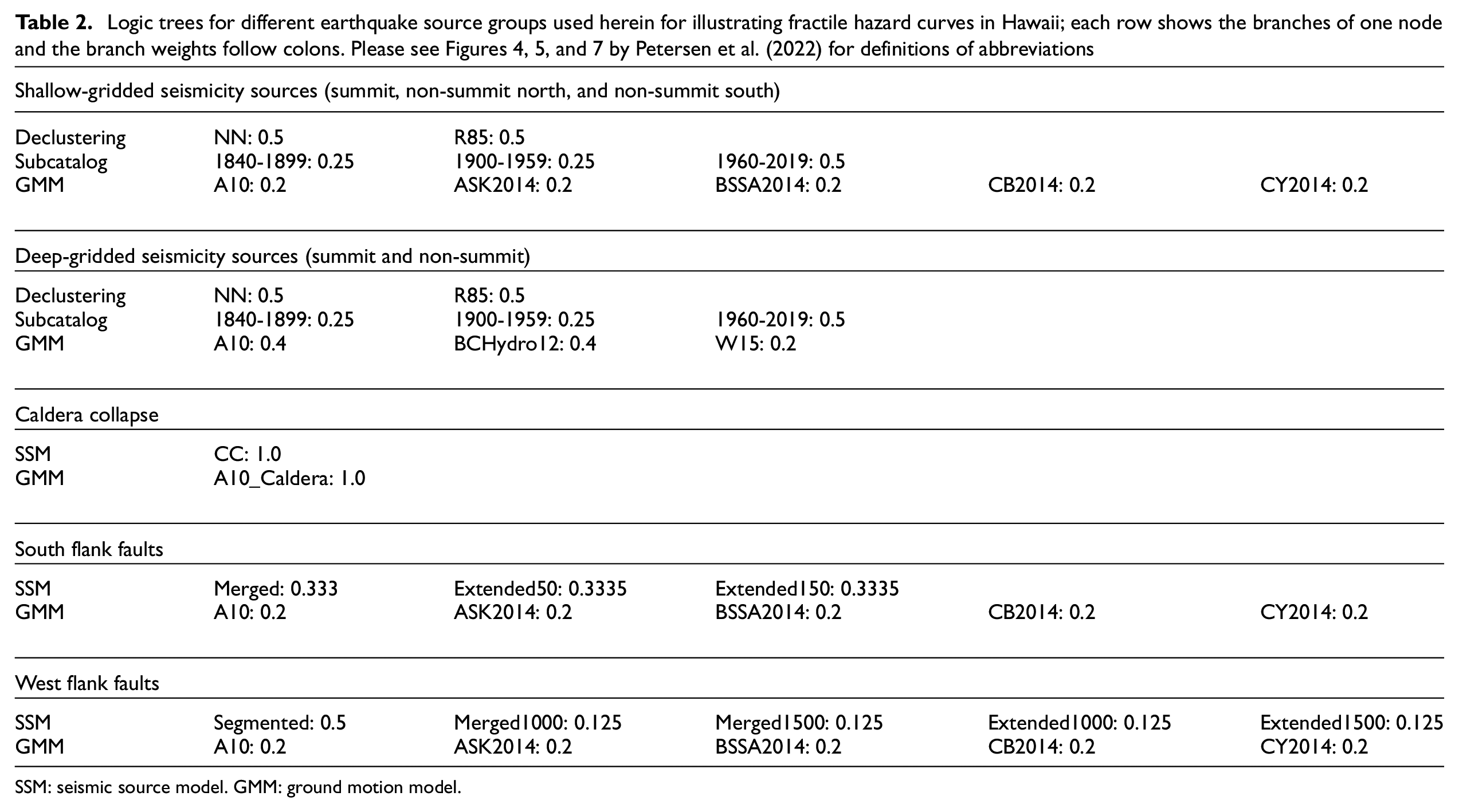
SSM: seismic source model. GMM: ground motion model.

To overcome such computational challenges when determining fractile hazard curves, we used Monte Carlo simulation instead. Specifically, we used the logic tree branch weights shown in Table 2 to independently simulate one realization of hazard curve from each of the eight source types. Then, the eight simulated hazard curves are added together to produce one corresponding realization of the total hazard curve. Repeating this process for a total of $n_{MC}$ simulations gives $n_{MC}$ realizations of total hazard curves for the given location and type of intensity measure. Because these simulated hazard curves were now generated from the underlying epistemic distributions shown in Table 2, the resulting fractile hazard curves may be determined by simply calculating the quantiles from the individual $n_{MC}$ hazard curves.

We explored different choices for $n_{MC}$ and found that for a specified level of precision, a greater number of simulations is required to estimate the 5th or 95th fractiles than the 15th or 85th fractiles. Similarly, a greater number of simulations is required to estimate the epistemic uncertainty in hazard at larger intensity measure levels than smaller intensity measure levels to the same level of precision. Based on exploration of stability of probabilistic ground motions with respect to choices of $n_{MC}$ , subsequent results shown are for $n_{MC} = 5 \times 10^{4}$ simulated hazard curves.

Figure 2 presents fractile hazard curves for Hilo and Honolulu and for SA(0.2) and SA(1.0). In total, we considered the same five locations in Hawaii that were studied by Petersen et al. (2022): (1) Hilo (19.7, −155.06), (2) Honolulu (21.3, −157.86), (3) Kahului (20.9, −156.5), (4) Kailua Kona (19.66, −156.0), and (5) Līhu‘e (21.96, −159.36). For a given location and type of intensity measure, the shaded region illustrates the range of the individual 50,000 simulated hazard curves.

Figure 2.

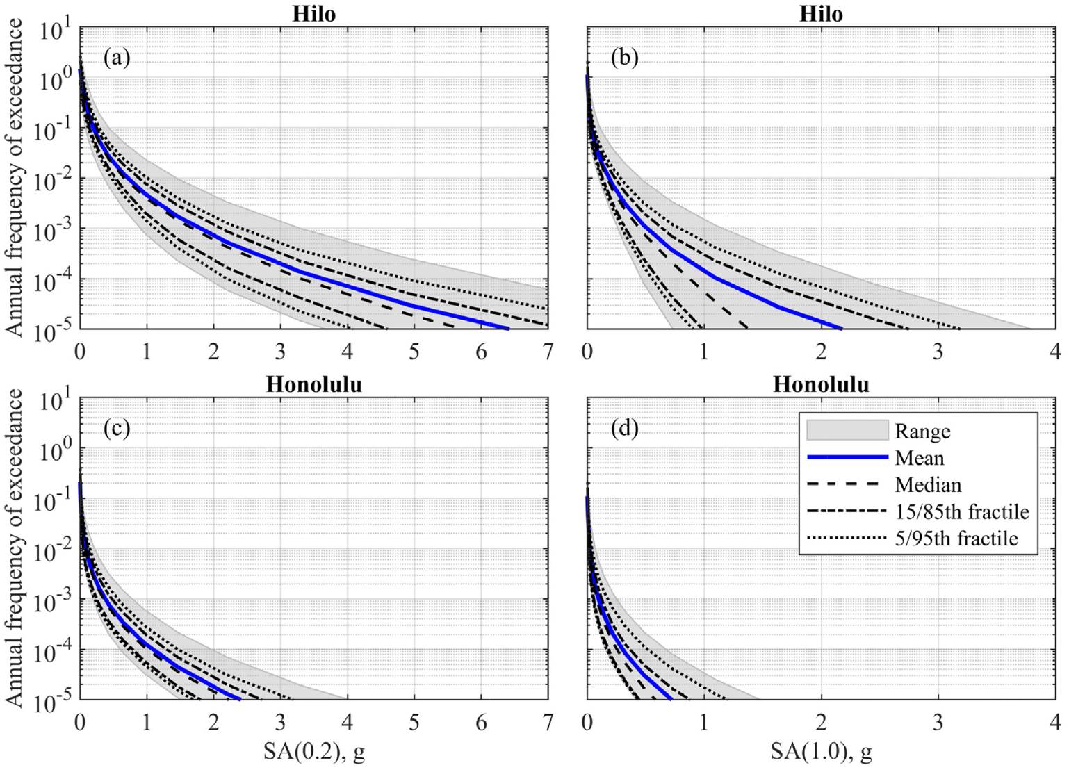
Mean and fractile hazard curves from USGS 2021 NSHM for example locations in Hawaii: (a) SA(0.2) in Hilo, (b) SA(1.0) in Hilo, (c) SA(0.2) in Honolulu, and (d) SA(1.0) in Honolulu.

A few comments can be made from the results that were used to create Figure 2. First, the fractile hazard curves, which include the median hazard curve, are determined by calculating the quantiles from the individual $n_{MC}$ hazard curves, instead of using Equations 1 –3 with the logic tree branch weights. Second, the mean exceeds the median for all AFEs, which indicates $F_{λ}$ is positively skewed; this differs from the previous results for California in which the positive skewness was observed only for low AFEs. Third, the epistemic uncertainty in AFE increases for decreasing AFE (increasing return period), which was also observed from the results for California. Fourth, distinct groups of individual branch AFEs can sometimes be observed at very small AFEs (very long return periods), which indicates that $F_{λ}$ might be poorly approximated by a lognormal distribution at very large intensity measure levels (e.g. SA(1.0) in Hilo at very small AFEs). Finally, similar to the results for California, the mean never exceeded the 85th fractile for the cases considered herein. In the next section, we synthesize lessons learned from both California and Hawaii to characterize the nature of epistemic uncertainty in the hazard and develop models for readily generating approximate fractile hazard curves.

Characterizing epistemic uncertainty in the hazard

The previous section illustrated two approaches for estimating fractile hazard curves; those in California were determined from Equations 1 –3, whereas those in Hawaii were determined from Monte Carlo simulation. For each state, the same master logic tree was used for all locations within the state (i.e. Table 1 for California and Table 2 for Hawaii). Because estimation of fractile hazard curves for one location required analyzing a relatively large number of individual branch hazard curves, reporting fractile hazard curves is fraught with computational challenges such as runtimes and memory storage. These observations indicate that it may be useful to develop a way to readily generate approximate fractile hazard curves.

Although the epistemic CDF of AFE at a fixed intensity measure level, $F_{λ}$ , might not follow a lognormal distribution strictly, the lognormal assumption has been used in past studies and has facilitated capturing of the center, body, and range of epistemic uncertainty (Atkinson et al., 2014; Bradley, 2009; Lee et al., 2018). In this article, we compared $F_{λ}$ against a lognormal approximation for all locations, intensity measure types, and intensity measure levels. We found that the epistemic distribution tends to be positively skewed and the mean tends to exceed the median. Furthermore, the lognormal approximation tends to be reasonable for most of the cases considered, with the approximation sometimes less reasonable at very small AFEs (very long return periods). Therefore, one way to explicitly quantify the epistemic uncertainty in AFE is to calculate the standard deviation of the (natural) logarithm of AFEs from individual hazard curves, $σ_{\ln λ} (im)$ .

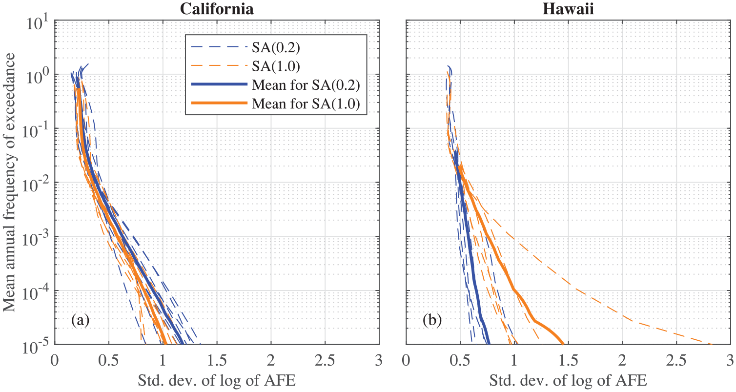
Figure 3 compares such epistemic logarithmic standard deviations against the corresponding mean AFEs, $\bar{λ} (im)$ . Specifically, Figure 3a presents eight curves of $\bar{λ}$ versus $σ_{\ln λ}$ that correspond to the eight locations in California; the curves for SA(0.2) are shown in blue, whereas those for SA(1.0) are shown in orange. For each intensity measure type, the solid line denotes the arithmetic mean of the standard deviations for a given value of mean AFE. Figure 3b presents similar $\bar{λ}$ versus $σ_{\ln λ}$ relations for the five locations in Hawaii; arithmetic means are computed only when data for all locations are available (e.g. the largest mean AFE at Līhu‘e is less than 1 × 10⁻¹).

Figure 3.

Mean annual frequency of exceedance (AFE) versus epistemic standard deviations of logarithm of AFE: (a) all eight sites in California and (b) all five sites in Hawaii.

A few observations can be made from the results shown in Figure 3. First, we observe that $σ_{\ln λ}$ tends to increase for decreasing mean AFEs (increasing return periods), which is consistent with observations from the literature. However, the precise relation between $\bar{λ}$ and $σ_{\ln λ}$ varies with the type of intensity measure, especially for Hawaii than for California. Second, we observe that unlike exceedance probabilities, the focus on AFEs enables quantification of epistemic uncertainty in hazard for very small intensity measure levels (i.e. epistemic uncertainty in earthquake occurrence). In fact, the $\bar{λ}$ versus $σ_{\ln λ}$ relation tends to approach a vertical line in the region of very large mean AFEs (i.e. constant $σ_{\ln λ}$ ). Therefore, the dependence on intensity measure type reduces for increasing mean AFE (decreasing return period) because epistemic uncertainty in earthquake occurrence is theoretically independent of the intensity measure type.

To better understand the trends, we directly compared the mean curves from each state against each other as shown in Figure 4. For SA(0.2), the epistemic uncertainty in AFE is larger for Hawaii than for California at mean AFEs larger than 2 × 10⁻³ (return periods shorter than 500 years) but then the trend reverses at smaller mean AFEs (Figure 4a). By contrast, for SA(1.0), the epistemic uncertainty in AFE is larger for Hawaii than for California across all mean AFEs (Figure 4b). The fact that the epistemic uncertainty in AFE is generally larger for Hawaii than for California at mean AFEs greater than 1 × 10⁻¹ makes sense because (1) this range of mean AFEs essentially corresponds to annual frequency of earthquake occurrence (e.g. Baker et al., 2021: 265) and (2) occurrence of earthquakes are less well studied in Hawaii than in California.

Figure 4.

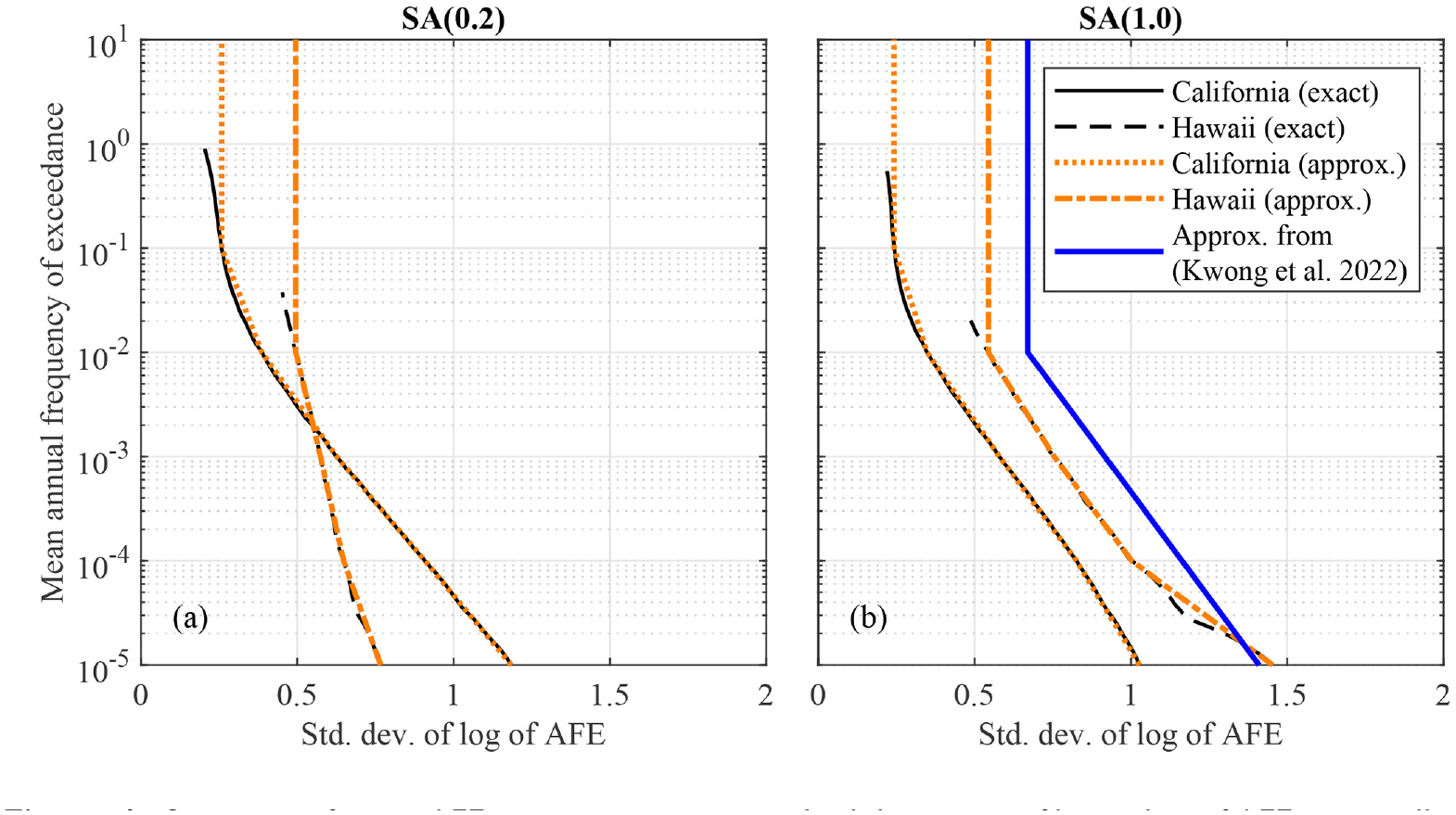
Summary of mean AFE versus epistemic standard deviations of logarithm of AFE across all sites: (a) SA(0.2) and (b) SA(1.0).

Based on the mean curves shown in Figure 4, we developed models for generating approximate fractile hazard curves. Such approximate fractile hazard curves are not a substitute for exact fractile hazard curves but would be useful for locations in which the latter are unavailable. First, we provide the numerical estimates of $σ_{\ln λ}$ at discrete values of mean AFE as shown in Table 3. For mean AFEs larger than 1 × 10⁻¹, the constant value of $σ_{\ln λ}$ at 1 × 10⁻¹ is used. In contrast, for mean AFEs smaller than 1 × 10⁻⁵, linear extrapolation in semi-log space is used. These approximations are shown as orange curves in Figure 4, along with the approximate relation for SA(1.0) in solid blue by Kwong et al. (2022).

Table 3.

Epistemic logarithmic standard deviations of AFE for generating approximate fractile hazard curves; for mean AFEs greater than 1 × 10⁻¹, the constant value at 1 × 10⁻¹ is used whereas for mean AFEs less than 1 × 10⁻⁵, linear interpolation in semi-log space is used (log of mean AFE versus standard deviation)

Mean AFE	Epistemic logarithmic standard deviation of AFE, $σ_{\ln λ}$
	California		Hawaii
	SA(0.2)	SA(1.0)	SA(0.2)	SA(1.0)
≥ 10⁻¹	0.26	0.24	0.50	0.54
10⁻²	0.39	0.35	0.50	0.54
10⁻³	0.63	0.58	0.57	0.75
10⁻⁴	0.91	0.83	0.65	1.00
10⁻⁵	1.18	1.03	0.77	1.45

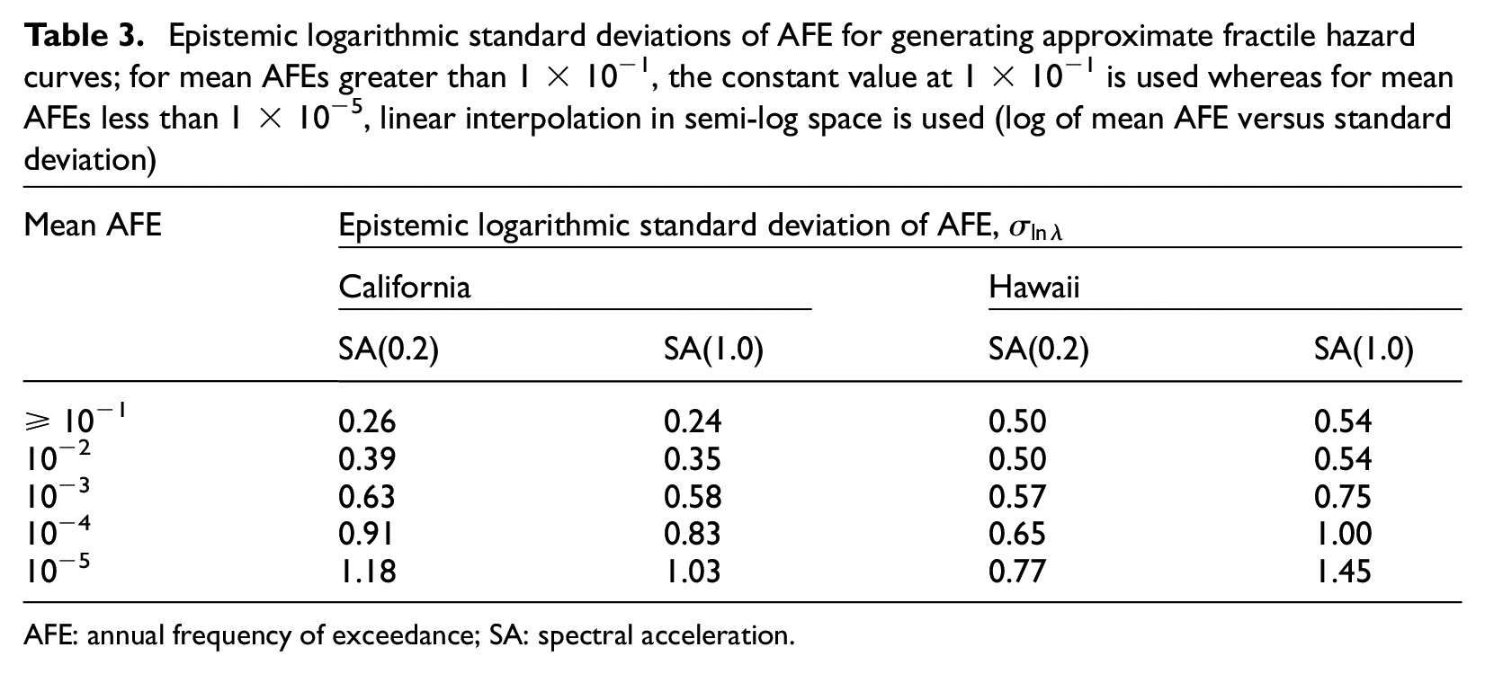
AFE: annual frequency of exceedance; SA: spectral acceleration.

In the study by Kwong et al. (2022), a relatively crude model for generating approximate fractile hazard curves was developed to understand the influence of various sources of uncertainty within a nationwide seismic risk assessment of gas transmission pipelines. Although that study had a different goal than this study, comparison of the approximate models in Figure 4b yields several observations. First, the trend of increasing $σ_{\ln λ}$ for decreasing mean AFE is again observed independently in this study. Furthermore, the relation between $\bar{λ}$ and $σ_{\ln λ}$ from Kwong et al. (2022) is closer to that of Hawaii than that of California. This observation makes sense because the model therein was intended for hazard curves at locations throughout the conterminous United States (CONUS) that are less well studied than those from California.

We propose to generate approximate fractile hazard curves using the simple approach from Kwong et al. (2022), but with estimates of standard deviations from Table 3 instead of those described therein. First, $F_{λ}$ is assumed to follow a lognormal distribution. Using an input mean hazard curve, $\bar{λ} (im)$ , Table 3 yields corresponding estimates of $σ_{\ln λ}$ that also vary with $im$ . Therefore, the $f$ th fractile can be readily approximated by multiplying the mean hazard curve as follows:

λ_{IM, f} (im) \approx \bar{λ} \cdot \exp [Φ^{- 1} (f) σ_{\ln λ} - 0.5 σ_{\ln λ}^{2}]

(4)

where $Φ^{- 1} (f)$ denotes the inverse of the standard normal CDF at the specified $f$ th fractile. Such approximate fractile hazard curves will be used in some of the subsequent examples.

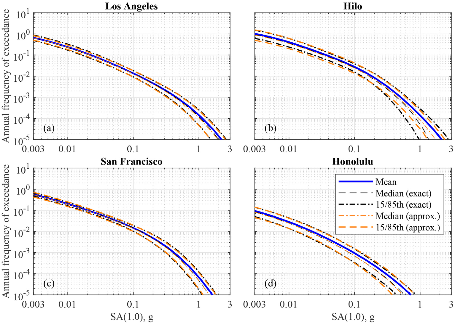
Figure 5 compares the approximate fractile hazard curves against the more exact fractile hazard curves for SA(1.0) at four locations. The agreement is excellent for a large range of AFEs, but the agreement can become poor at very small AFEs (e.g. smaller than 4.04 × 10⁻⁴ for SA(1.0) in Hilo). Such occasional poor agreement is due to $F_{λ}$ deviating from lognormality. For risk analyses in which small AFEs are of interest, more exact fractile hazard curves should be used, and if approximate fractile hazard curves are used instead, caution should be exercised when interpreting results from such risk analyses.

Figure 5.

Approximate versus more exact fractile hazard curves for SA(1.0) at: (a) Los Angeles, (b) Hilo, (c) San Francisco, and (d) Honolulu.

To further characterize the epistemic uncertainty in hazard, we examine the correlation between the logarithm of AFE at two different intensity measure levels. We denote the two different intensity measure levels using $i m_{i}$ and $i m_{j}$ ; we denote the correlation using $ρ$ . By comparing the correlations against the corresponding ratios of the two intensity measure levels (i.e. $ρ$ versus $(i m_{j} / i m_{i})$ ), correlation relations from different locations and intensity measure types can be directly compared against each other (Bradley, 2009). These correlation relations are plotted in Figure 6; each individual curve corresponds to one location and one intensity measure type. For each curve, correlation coefficients are estimated for many different pairs of intensity measure levels; then, these data are used to determine the arithmetic average correlation coefficient for a given ratio of intensity measure levels, resulting in a curve of $ρ$ versus $(i m_{j} / i m_{i})$ . For each state, the curves are colored based on intensity measure type; the arithmetic average (across both intensity measure types and all locations) is illustrated in solid black and for reference, the correlation model from Bradley (2009) is also illustrated in solid gray.

Figure 6.

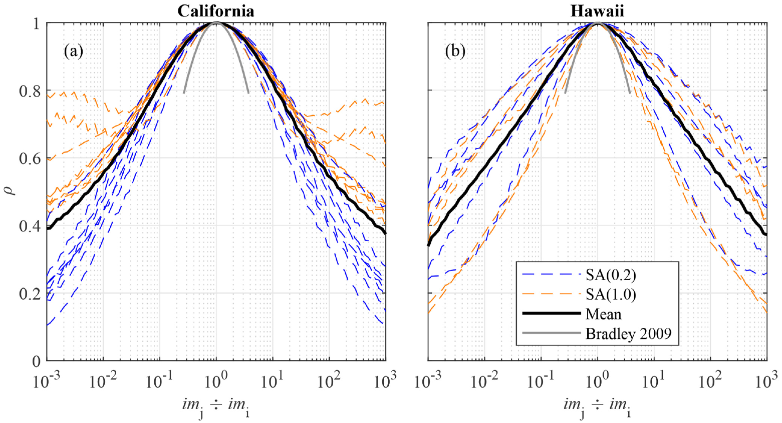
Correlation between logarithms of AFE at two different intensity measure levels as a function of the ratio between the two levels: (a) California and (b) Hawaii.

Figure 6a shows that in California, the correlation relation is relatively insensitive to both location and type of intensity measure when the two intensity measure levels are close to each other. For instance, when the two intensity measure levels are identical to each other, the correlation equals unity. By contrast, when the two intensity measure levels are very far apart from each other (e.g. ratio of 1 × 10³), the correlation relation depends strongly on the type of intensity measure and location; specifically, the correlation is stronger for SA(1.0) than SA(0.2).

Figure 6b shows that unlike California, the correlation relation for Hawaii differs in two major ways. First, when the two intensity measure levels are close to each other, the correlation relation is more sensitive to location in the case of Hawaii than in the case of California. Second, the correlation relation is relatively insensitive to the type of intensity measure, regardless of the ratio between the two intensity measure levels.⁶

Although the correlation relation generally varies with both location and type of intensity measure, it may still be useful to approximate such correlations for estimating the epistemic joint distribution (e.g. epistemic bivariate distribution of log of AFE at two different intensity measure levels) in the context of uncertainty propagation (Bradley, 2009; McGuire et al., 2005). For example, the correlation model by Bradley (2009) was used in the semiparametric Monte Carlo approach to propagate epistemic uncertainty when estimating the probability of collapse for a hypothetical structure. Although Figure 6 shows that this correlation model underestimates the actual correlations for nearly all the cases considered herein, it should be noted that the model was developed using older data (UCERF2) and for a smaller geographical region (San Francisco Bay Area); nevertheless, the new data herein do confirm that the correlations are indeed closer to unity than to zero (see Figure 7 in Bradley, 2009). Considering correlation relations from all locations and both types of intensity measures, we developed the following model to approximate the correlation between the logarithm of AFE at two different intensity levels:

ρ = 1.0 - 0.04 {[\ln (\frac{i m_{\max}}{i m_{\min}})]}^{2} + 0.004 {[| \ln (\frac{i m_{\max}}{i m_{\min}}) |]}^{3} \frac{i m_{\max}}{i m_{\min}} \leq 10^{3}

(5)

where $i m_{\max}$ ( $i m_{\min}$ ) refers to the larger (smaller) intensity measure level among the two. Correlations from Equation 5 can be combined with standard deviations from Table 3 to estimate epistemic covariance in the hazard for uncertainty propagation. However, this approach requires consideration of the semipositive definiteness of the resulting covariance matrix.

Figure 7.

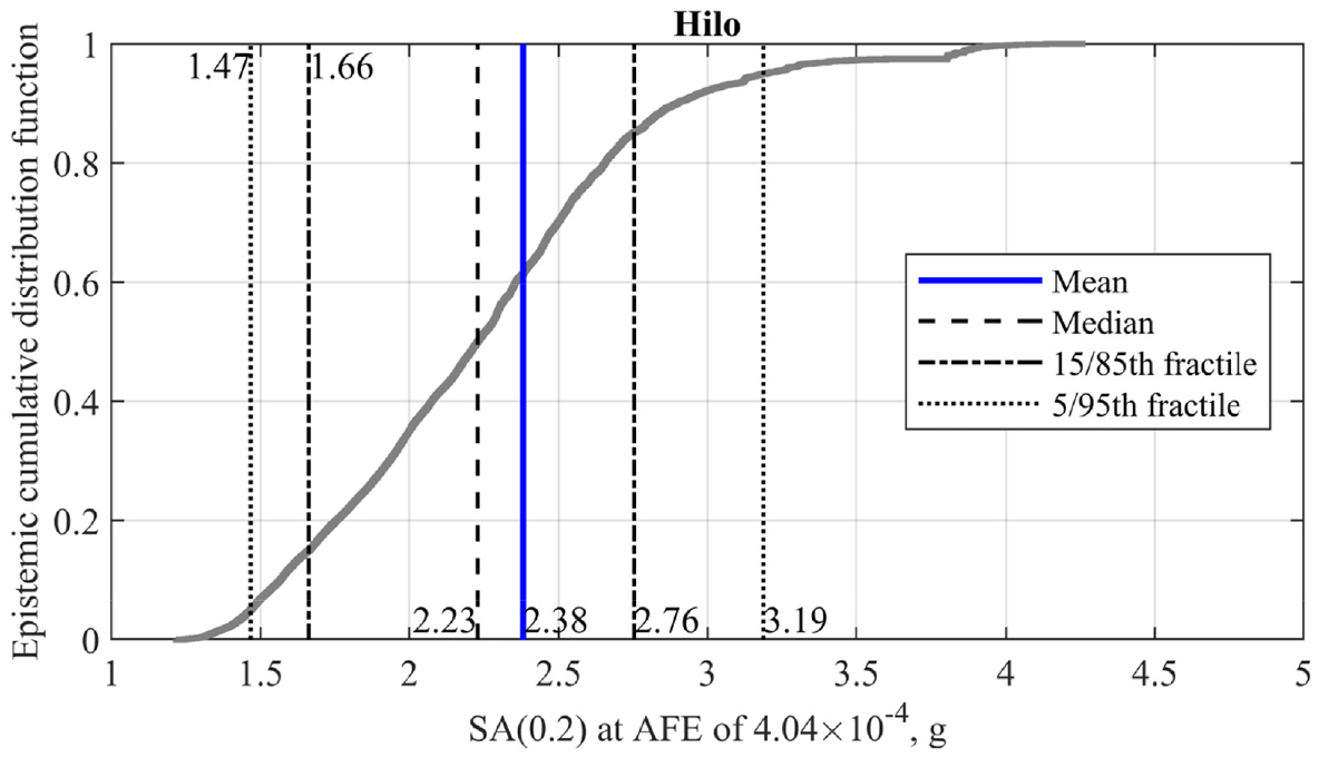
Example use of fractile hazard curves: determining confidence in UHGM for SA(0.2) in Hilo, at a specified AFE of $4.04 \times 10^{- 4}$ (return period of 2475 years).

Uses of fractile hazard curves

In this section, we used both approximate and more exact fractile hazard curves to illustrate a variety of potential downstream applications from reported epistemic uncertainties in the hazard. We intentionally kept the examples brief to showcase breadth rather than depth. To help readers more easily navigate this section, Table 4 summarizes the six examples.

Table 4.

Summary of examples for illustrating potential uses of fractile hazard curves

Ex. no.	Context	Description
1	Hazard	Determining confidence in UHGMs
2	Hazard	Visualizing epistemic uncertainty corresponding to UHGM maps
3	Hazard	Checking stability in mapped UHGMs over time across NSHM updates
4	Risk	Evaluating buildings that were designed from mean hazard
5	Risk	Propagating epistemic uncertainties in risk assessments of bridges
6	Risk	Comparing sources of uncertainties when assessing risks to pipelines

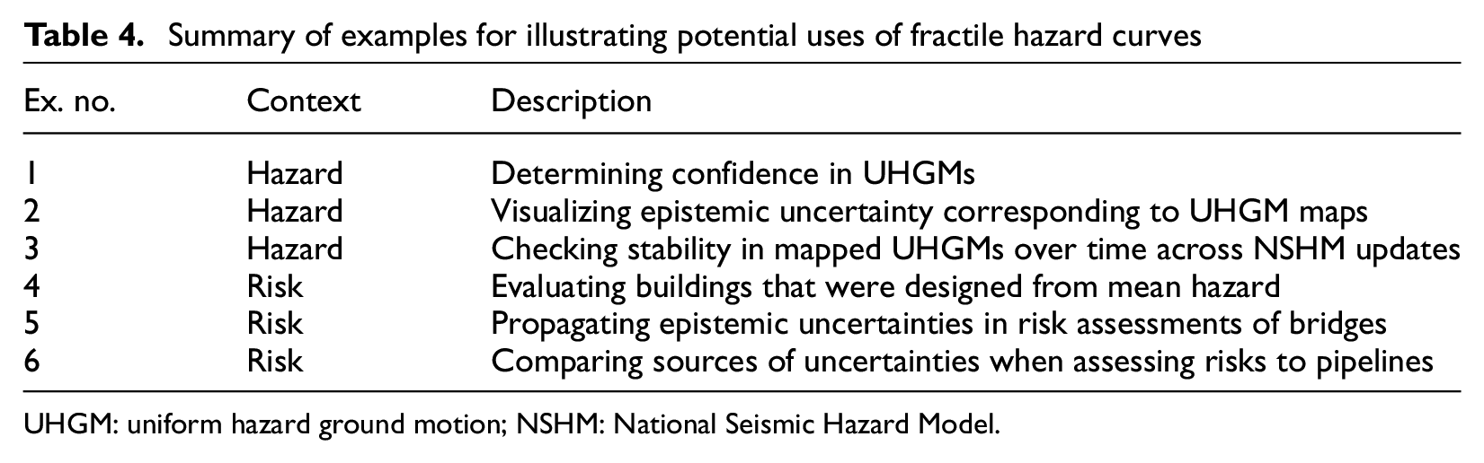
UHGM: uniform hazard ground motion; NSHM: National Seismic Hazard Model.

Hazard example 1

One use of fractile hazard curves is for determining confidence in the probabilistic ground motion or uniform hazard ground motion (UHGM) that was derived from mean hazard. For example, the blue vertical line in Figure 7 illustrates the UHGM for SA(0.2) in Hilo, at a specified AFE of 4.04 × 10⁻⁴ (return period of 2475 years). Put differently, this UHGM was determined from the mean hazard curve in Figure 2a, using an input AFE of 4.04 × 10⁻⁴ (i.e. the uniform hazard).

Although the choice of AFE or return period quantifies the desired “safety level” (i.e. vertical direction in Figure 2a), the choice of fractile quantifies the desired “confidence level” (i.e. horizontal direction in Figure 2a) (Abrahamson and Bommer, 2005). At an AFE of 4.04 × 10⁻⁴ (return period of 2475 years), the UHGMs corresponding to five fractiles are also illustrated in Figure 7 using different line styles in black color. Furthermore, the empirical CDF from all 5 × 10⁴ values of the UHGM is shown in solid gray; this quantifies the epistemic uncertainty in UHGM, not the epistemic uncertainty in hazard, $F_{λ}$ . These data enable the determination of a confidence interval for the UHGM. For example, the 15th and 85th fractiles indicate an approximate 70% confidence interval for the UHGM of about 1.66g−2.76g, whereas the 5th and 95th fractiles indicate an approximate 90% confidence interval of about 1.47g−3.19g; these intervals provide more context for interpreting the reported mean value of 2.38g (g is gravitational acceleration at the surface of the Earth, about 9.8 m/s²). In passing, we note that the mean and 85th fractile are the same as those shown in Figure 17d by Petersen et al. (2022), but the other fractiles differ slightly primarily because all eight earthquake source types were used herein to determine the fractiles, whereas disaggregation was used to identify a subset of earthquake source types by Petersen et al. (2022).

Hazard example 2

A second use of fractile hazard curves is for visualizing epistemic uncertainties that are inherent in maps of UHGMs. For example, Figure 8 illustrates the UGHM map for SA(1.0) in Hawaii, at a specified AFE of 4.04 × 10⁻⁴ (return period of 2475 years or 2% Poisson exceedance probability in 50 years). For each location in the map, the corresponding mean hazard curve was used to determine the resulting UHGM value; however, fractile hazard curves could also be used at each location.

Figure 8.

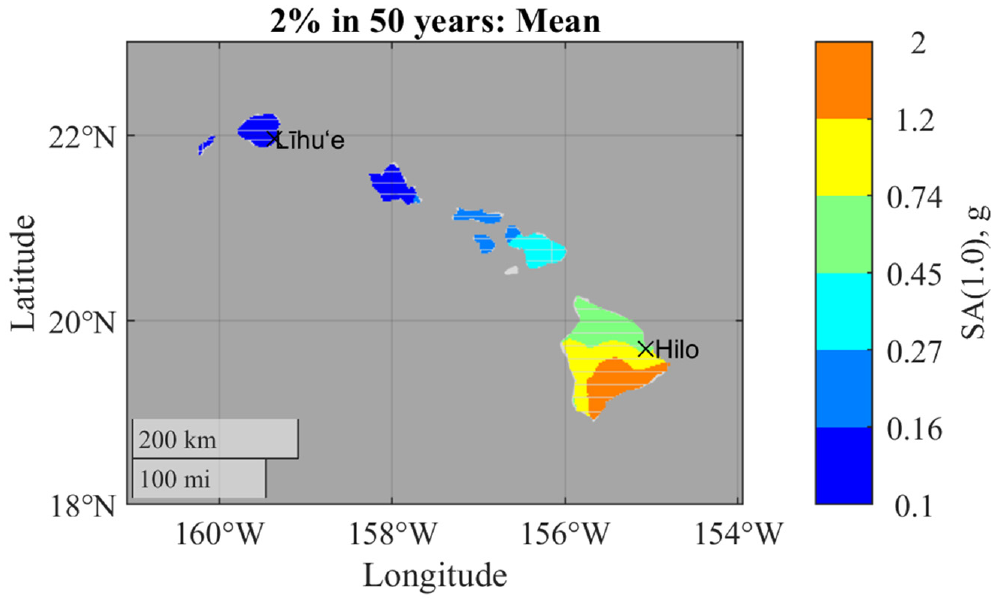
Mean-based UHGM map for 1.0-s spectral acceleration in Hawaii, at a specified AFE of 4.04 × 10⁻⁴ (return period of 2475 years).

Researchers have examined various ways to visualize uncertainties in a map (e.g. Schneider et al., 2022). For instance, one way is to plot the central estimates (e.g. means) directly adjacent to estimates of uncertainty (e.g. standard deviations). A second way is to illustrate the uncertainty through color transparency. In this alternative, the mean-based map is again shown, but regions with a color that is more transparent has larger epistemic uncertainty or less confidence (e.g. Retchless and Brewer, 2016).

A third way is to plot the lower bounds of a confidence interval directly adjacent to the upper bounds, using the same color scheme across the two plots (e.g. Nadav-Greenberg et al., 2008). For example, using the approximate fractile hazard curves that were described earlier, Figure 9a shows the map derived from the 15th fractile hazard curves at each location (i.e. lower bound), whereas Figure 9b shows the map derived from the 85th fractile hazard curves (i.e. upper bound). In this approach, similar colors across the two plots at a particular location indicate low epistemic uncertainty (e.g. high confidence of low hazard at Līhu‘e). By contrast, differing colors at a particular location indicate high epistemic uncertainty (e.g. lower confidence in the hazard at Hilo because of green color in Figure 9a versus yellow color in Figure 9b). In the context of aftershock forecast maps, Schneider et al. (2022) found that showing the lower/upper bounds was more effective than the other two approaches at communicating “potential surprise” locations (i.e. locations where high uncertainty could lead to worse outcomes than predicted). Like the mean-based UHGM map in Figure 8, the fractile-based UHGM maps in Figure 9 are not physically realizable because the ground motion value at one location is determined independently from that at another location. Therefore, although Figure 9 helps distinguish different degrees of confidence in the mapped values from Figure 8, all three maps should not be used in loss or risk assessments that require spatial correlation of ground motions (e.g. regional risk assessment of spatially distributed infrastructure).

Figure 9.

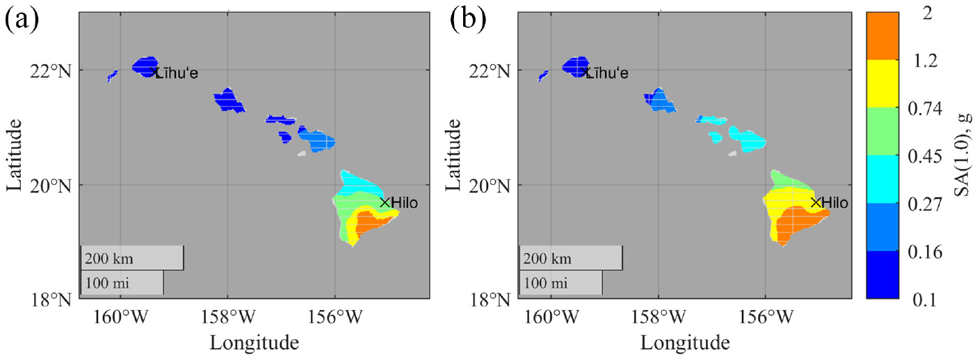
Example use of fractile hazard curves: visualizing epistemic uncertainty in UHGM map for SA(1.0) in Hawaii, at a specified AFE of 4.04 × 10⁻⁴ (return period of 2475 years): (a) 15th fractile and (b) 85th fractile.

Hazard example 3

A third use of fractile hazard curves is for checking stability in mapped UHGMs over time across NSHM updates. For example, the blue circles in Figure 10a illustrate UHGMs for SA(1.0) in Los Angeles from the three most recent updates of the USGS NSHM, at a specified AFE of 4.04 × 10⁻⁴ (return period of 2475 years). Similarly, the blue circles in Figure 10b illustrate UHGMs for SA(1.0) in Hilo from the two most recent updates of the USGS NSHM. These fluctuations over time could potentially convey a lack of stability in the mapped values (Hamburger et al., 2017); however, how “big” or “small” are such fluctuations?

Figure 10.

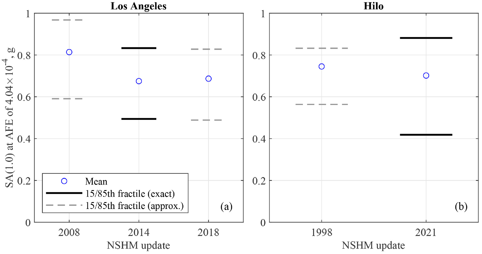
Example use of fractile hazard curves: checking stability in mapped UHGMs over time across USGS NSHM updates; SA(1.0) at a specified AFE of 4.04 × 10⁻⁴ (return period of 2475 years) in (a) Los Angeles and (b) Hilo.

The fractile hazard curves could be used to gain insight to this question. For example, the 15th and 85th fractile-based UHGMs that correspond to each mean value are also shown in Figure 10. For the 2014 and 2021 updates, the fractile-based UHGMs are illustrated using solid black lines, whereas those for the other updates are illustrated using dashed gray lines; this was done to convey that the latter were estimated from approximate fractile hazard curves (Equation 4). In contrast, the 2014 values for Los Angeles correspond to those shown in Figure 1b, while the 2021 values for Hilo correspond to those shown in Figure 2b.

Comparison of the confidence intervals between the 2018 and 2014 updates for Los Angeles indicates that the mapped values across the two updates appear to be stable, even though the latest mapped value increased by about 2%. This makes sense because the only major change for this location between these two updates was the addition of a basin model (Petersen et al., 2020). Similarly, comparison of the confidence intervals between the 2021 and 1998 updates for Hilo indicates that the mapped values across the two updates also appear to be stable, even though the latest mapped value decreased by about 6%. In contrast, the noticeable decrease in confidence interval for Los Angeles from the 2008 update to the 2014 update is consistent with the approximate 20% decrease in the mapped value, which may prompt investigation of the reasons behind such discrepancies. Further investigation reveals that a major difference for this location between these two updates was a major change in the hazard modeling process, from UCERF2 to UCERF3 (Field et al., 2014; Petersen et al., 2015). Finally, the confidence interval for each update could potentially be used as a basis for averaging mapped values from several updates in an effort to stabilize ground motion values for engineering design⁷ (Hamburger et al., 2017).

Risk example 1

In the context of risk, one example use of fractile hazard curves is for evaluating buildings that were designed from mean hazard. For example, Figure 11 illustrates the determination of risk-targeted ground motions (RTGMs) for designing a hypothetical building in Los Angeles (Luco et al., 2007). The solid black curve in Figure 11a shows the mean hazard curve for SA(1.0) in Los Angeles and a UHGM value of 0.68g, at a specified AFE of 4.04 × 10⁻⁴ (return period of 2475 years). On the contrary, the solid black curve in Figure 11b shows the corresponding risk-targeted fragility curve that was derived (see Appendix 1) from risk targets of (1) 1% probability of collapse in 50 years (i.e. AFE of 2.01 × 10⁻⁴ or return period of 4975 years) and (2) 10% conditional probability of collapse given the RTGM value (Haselton et al., 2017). Corresponding to the 15th, mean, and 85th fractile hazard curves, Figure 11a also shows the UHGMs and Figure 11b also shows the RTGMs. Unlike the UHGM value of 0.68g, the RTGM value of 0.61g incorporates the fragility of a building (i.e. consequences beyond hazard) and, hence, enables designs based on uniform risk rather than uniform hazard. However, the RTGM is about 10% smaller than the UHGM. Because both values of GM were derived from the mean hazard curve, they both contain epistemic uncertainty. Therefore, it may be cost-effective to intentionally design to a level higher than what is required by regulations to account for potential retrofit mandates caused by future revisions of seismic hazard estimates (e.g. revision of logic tree branches for new GMMs) (McGuire et al., 2005).

Figure 11.

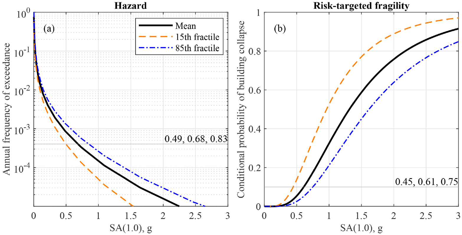
Example use of fractile hazard curves: evaluating a hypothetical building in Los Angeles that was designed from mean hazard: (a) hazard curves (with UHGMs shown) and (b) corresponding risk-targeted fragility curves (with RTGMs shown) from assuming an aleatory logarithmic standard deviation of $β_{R} = 0.6$ ; risk targets defined as 1% probability of building collapse in 50 years and 10% conditional probability of building collapse given the design GM.

One potential way to develop confidence in a mean-based design is to evaluate the design using a UHGM that was derived from a high fractile hazard curve. For example, the blue chained curve in Figure 11a shows the 85th fractile, with a corresponding UHGM value of 0.83g. The UHGM value of 0.83g might be used instead of the mean value of 0.68g to conduct disaggregation, perform nonlinear response history analyses, and check design acceptance criteria (Zimmerman et al., 2017). If the mean-based design remains satisfactory even under a more intense ground motion, one can be more confident that the design (1) achieves the objectives that were originally intended and (2) offers better functional performance (e.g. “immediate occupancy” instead of “life safety”; Moehle and Deierlein, 2004) than a design that is barely satisfactory at the mean hazard.

Another potential way to develop confidence in a mean-based design is to evaluate it using an RTGM that was derived from a high fractile hazard curve. For example, the blue chained curve in Figure 11b shows the risk-targeted fragility resulting from use of the 85th fractile hazard curve instead of the mean hazard curve (see Appendix 1). Although the risk targets remain the same as before, the resulting risk-targeted fragility median is now increased because the input hazard is now higher. Consequently, the 85th fractile-based RTGM value of 0.75g exceeds the mean-based RTGM value of 0.61g. As before, this higher RTGM value might be used to initiate evaluation of a mean-based design.

Although Figure 11 illustrates the potential of evaluating a design with a “high” fractile hazard curve, what constitutes as “high” depends on the specific problem under consideration. For example, designing nuclear facilities may require consideration of very low AFEs (e.g. 1 × 10⁻⁷ or lower), and hence, the mean might exceed the 85th fractile (Abrahamson and Bommer, 2005). However, we note that (1) it is not surprising for the mean to exceed a given fractile (e.g. the mean exceeded the median in earlier examples), and (2) a higher fractile that exceeds the mean can always be considered (e.g. 95th fractile).

Risk example 2

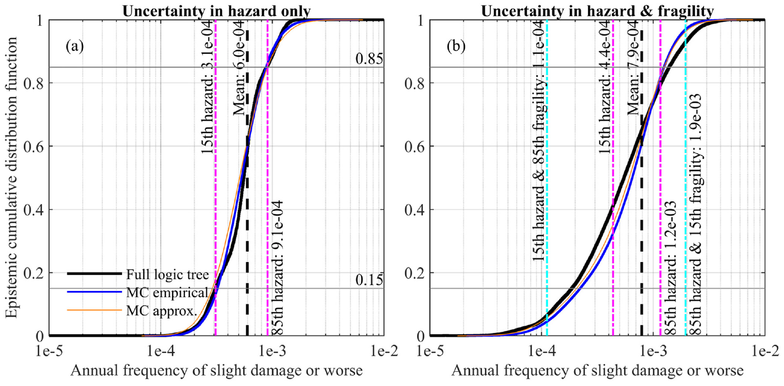
Fractile hazard curves can also be used for propagating epistemic uncertainties in site-specific seismic risk assessments. As an example, suppose that one is interested in estimating the annual frequency of exceeding slight damage, $λ_{slight}$ , for a hypothetical highway bridge in Los Angeles (Jaiswal et al., 2020). Using the mean hazard curve for SA(1.0) (Figure 1b) and the default fragility function for a Hazus highway bridge class of HWB28 (i.e. a generic, unclassified bridge; Federal Emergency Management Agency (FEMA), 2022), it can be readily shown (see Appendix 1) that the resulting annual frequency of exceeding slight damage is about $λ_{slight} = 6 \times 1 0^{- 4}$ . However, this risk estimate contains epistemic uncertainty because the input hazard curve, $λ_{IM} (im)$ , also contains epistemic uncertainty (Figure 1b).

Multiple approaches are available to propagate epistemic hazard uncertainties in site-specific risk assessments (e.g. Bradley, 2009), and we consider three approaches herein. In the first approach (“Full logic tree”), the risk calculation is repeated for each of the individual 21,600 hazard curves that correspond to the full logic tree, leading to an epistemic empirical CDF of $λ_{slight}$ . In the second approach (“MC empirical”), the preceding 21,600 hazard curves are replaced by $n_{MC}$ hazard curves from Monte Carlo simulation of the epistemic joint distribution of the hazard curve, $λ_{IM} (im)$ . Specifically, the hazard curve is assumed to follow a multivariate lognormal distribution, with median vector and covariance matrix estimated empirically from the original 21,600 hazard curves. The third approach (“MC approx.”) is identical to the second approach except for the parameters of the multivariate lognormal distribution; in this case, the median vector and covariance matrix are approximated by standard deviations from Table 3, median from Equation 4, and assuming perfect correlation $(ρ = 1)$ across the intensity measure levels. For each of these three approaches, we consider both exclusion of epistemic uncertainty in the fragility (i.e. uncertainty in hazard only) as well as inclusion of this uncertainty; specifically, we use a double-lognormal model with an epistemic logarithmic standard deviation of $β_{U} = 0.4$ (see Appendix 1).

Assuming no epistemic uncertainty in the fragility, Figure 12a compares the empirical CDF of $λ_{slight}$ from the preceding three approaches against the mean value of $λ_{slight}$ from combining the mean hazard curve with the unique fragility curve, which is shown by a black dashed vertical line. This mean value is almost identical to the mean values from all three approaches of propagating epistemic uncertainties, which highlights the “invariance” of using the mean hazard in decision-making (McGuire et al., 2005). However, the comparison of propagation approaches demonstrates that for this hypothetical bridge, the annual frequency of exceeding slight damage is not just 6 × 10⁻⁴, but likely somewhere between 1 × 10⁻⁴ and 2 × 10⁻³. Furthermore, the mean exceeds the medians from all three approaches, implying that the epistemic distribution of $λ_{slight}$ is positively skewed.

Figure 12.

Example use of fractile hazard curves: propagation of epistemic uncertainties in a site-specific seismic risk assessment of an unclassified highway bridge in Los Angeles: (a) no epistemic uncertainty in fragility and (b) fragility median assumed to follow a lognormal distribution with an epistemic logarithmic standard deviation of ${beta}_{U} = 0.4$ .

The agreement between the “MC empirical” and “Full logic tree” approaches is excellent, confirming the earlier assertion that the epistemic uncertainty in hazard can be reasonably approximated by a lognormal distribution for most of the cases considered. The “MC approx.” approach is simpler to implement than the “MC empirical” approach because the former requires only the mean hazard curve and standard deviations from Table 3, whereas the latter requires all 21,600 hazard curves from the full logic tree.

All three approaches yield roughly similar estimates of the 15th and 85th epistemic percentiles of $λ_{slight}$ , with “MC empirical” more accurate than “MC approx.” (Figure 12a). However, all three approaches required thousands of repeated risk calculations—one for each individual hazard curve. In contrast, simply repeating the risk calculation twice, once using the 15th fractile and a second time using the 85th fractile, gives excellent agreement to the confidence intervals from the other approaches (chained magenta lines in Figure 12a). However, when epistemic uncertainty in fragility is also included in the propagation, combining the fractile hazard curves with the mean fragility curve underestimates the actual epistemic uncertainty in $λ_{slight}$ (chained magenta lines in Figure 12b).

Figure 12b also illustrates several more effects from including epistemic uncertainty in the fragility. First, the epistemic uncertainty in risk increases (i.e. range increases from roughly [9 × 10⁻⁵, 2 × 10⁻³] in Figure 12a to roughly [1 × 10⁻⁵, 4 × 10⁻³] in Figure 12b). Second, the mean estimate also increases from about 6 × 10⁻⁴ to 8 × 10⁻⁴. Third, the mean from combining the mean hazard with mean fragility is the same as the mean from the “Full logic tree” approach, whereas the means from the Monte Carlo approaches are slightly smaller. Fourth, the new mean estimates of $λ_{slight}$ in Figure 12b remain larger than the corresponding medians and, hence, the new epistemic CDF of $λ_{slight}$ remains positively skewed. Finally, instead of combining the mean fragility curve with the 15th and 85th fractile hazard curves, combining the 15th and 85th hazard curves with the 85th and 15th fractile fragility curves,⁸ respectively, provides a conservative approximation of the 70% confidence interval for $λ_{slight}$ (chained cyan in Figure 12b).

Risk example 3

A final illustrative use of fractile hazard curves is for comparing epistemic uncertainties in hazard against other types of uncertainties within a seismic risk assessment. For example, a recent study on seismic risk of gas transmission pipelines in the CONUS integrated four key models when estimating average annual loss: (1) hazard (USGS 2018 NSHM), (2) exposure (locations and attributes of pipelines), (3) vulnerability (relation between rate of pipeline leaks or breaks and intensity measure), and (4) consequence (costs required to physically repair leaks or breaks) (Kwong et al., 2022). Besides epistemic uncertainties in the hazard, uncertainties also existed for the other three models. Based on the uncertainties approximated therein, the study found that the vulnerability model was the most influential source of uncertainty in the seismic risk assessment, whereas the hazard model was the third most influential source. However, this conclusion was based on fractile hazard curves that were crudely approximated using published information from Stepp et al. (2001). Therefore, different input epistemic uncertainties in the hazard could potentially change the rankings in the tornado diagrams.

Figure 13 presents results from repeating the sensitivity analyses that were described by Kwong et al. (2022) but with different input fractile hazard curves. Specifically, Figure 13a presents the tornado diagram resulting from replacing the input fractile hazard curves with those generated from standard deviations for California shown in Table 3. By contrast, Figure 13b presents the tornado diagram resulting from application of the standard deviations for Hawaii shown in Table 3 instead. In both cases, the vulnerability model remained the most influential source of uncertainty when estimating AAL within the CONUS. However, the hazard model was the least influential source of uncertainty in Figure 13a, whereas it is the third-most influential source of uncertainty in Figure 13b. Therefore, implications from a given downstream application of hazard information could strongly depend on the input fractile hazard curves, and hence, epistemic uncertainties in the hazard should be carefully estimated.

Figure 13.

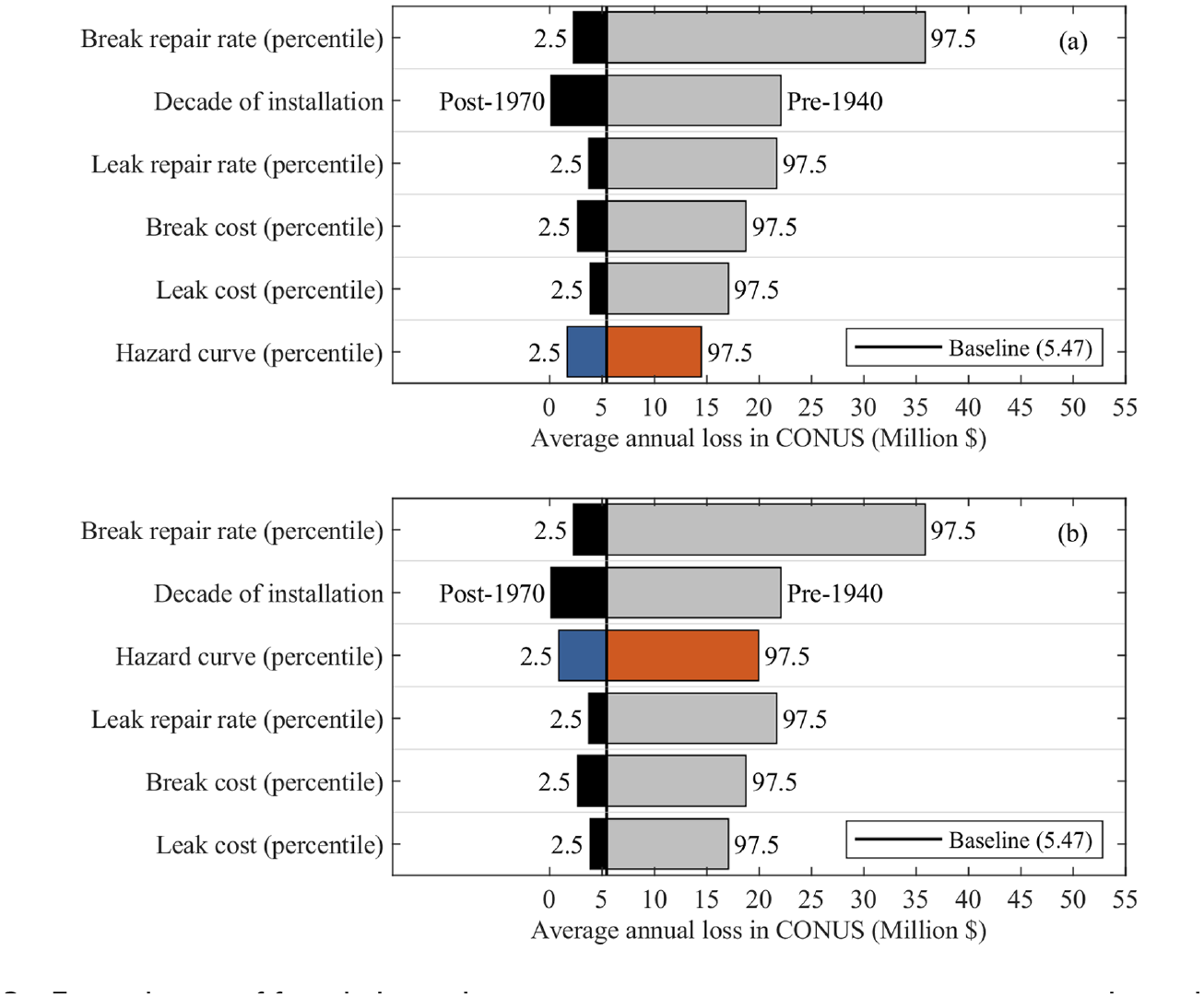
Example use of fractile hazard curves: comparing epistemic uncertainties in hazard against other types of uncertainties in a seismic risk assessment; tornado diagram for average annual loss of gas transmission pipelines in CONUS using (a) standard deviations for California from Table 3 and (b) standard deviations for Hawaii from Table 3.

Other potential uses of epistemic uncertainty in the hazard

The preceding six examples are intended to portray a variety of possible uses of fractile hazard curves and provide inspiration for other potential applications. Consequently, the uses are neither exhaustive nor comprehensive. For instance, Figure 7 illustrated the use of fractile hazard curves for determining confidence in the UHGM for SA(0.2) in Hilo, at a specified AFE of 4.04 × 10⁻⁴ (return period of 2475 years). However, yet another potential use of the epistemic uncertainties shown in Figure 7 is to quantify the epistemic uncertainty in the mean estimate of the UHGM. In this case, the mean estimate from Equation 1 would be viewed as a random variable with its own epistemic uncertainty. However, such quantification would require knowledge of not only the epistemic uncertainty in the AFE for a given logic tree branch (i.e. the variance of $λ_{k}$ ), but also the correlations between the hazard from various logic tree branches, which is a topic beyond the scope of this article.

In the context of risk, Figure 13 illustrated the use of fractile hazard curves for understanding the size of epistemic uncertainties in the hazard, relative to other sources of uncertainty. However, yet another potential use of such fractile hazard curves is to calibrate a set of earthquake rupture scenarios in the region so that spatial correlations of ground motions can be properly accounted for in regional seismic risk assessments of buildings and critical infrastructure systems (e.g. Lee et al., 2022; Miller and Baker, 2015; Soleimani et al., 2021). Furthermore, by more completely connecting all hazard uncertainties to various risk metrics, scientific efforts can be better prioritized with respect to reducing epistemic uncertainties (Field et al., 2020).

Given the wide variety of potential uses of epistemic uncertainties in hazard, we aimed to enable a broad range of users of USGS NSHMs to independently examine and potentially start using such epistemic uncertainties for their respective applications. To facilitate sensitivity analyses and encourage user engagement, we developed an open-source interactive tool that extends the second risk example described in this article, which can be accessed using Kwong and Jaiswal (2023). Specifically, we developed an accompanying Python-based Jupyter notebook that enables readers to try different input hazard curves when conducting a site-specific seismic risk assessment of a given hypothetical highway bridge (https://code.usgs.gov/ghsc/erp/bridge_risk_interactive_tool).

Figure 14 shows a screenshot of this tool, which is built upon the open-source HoloViews Python library (Stevens et al., 2015). For a given input hazard curve from a comma-separated value (CSV) file, the user can specify other inputs of the seismic risk assessment through widgets on the left (e.g. fractile, Hazus highway bridge class, damage state, epistemic logarithmic standard deviation of the fragility median). Examples of input hazard curves include, but are not limited to the following: (1) hazard curve for another location or for a different update cycle of the NSHM (Shumway et al., 2021), (2) hazard curve for a different estimate of $V_{S 30}$ , or (3) hazard curve corresponding to a specific logic tree branch. For each set of inputs, the tool automatically revises the resulting risk estimates (e.g. plots of input hazard curves and input fragility curves are automatically refreshed). Furthermore, the plots are interactive (e.g. can zoom or pan to determine precise numerical values) and dynamically linked (e.g. manipulation of the hazard plot automatically updates the fragility plot). To facilitate sensitivity analyses, risk estimates from user-specified inputs are automatically compared visually against baseline risk estimates; for a given input hazard curve, the corresponding baseline risk is estimated from the default inputs that are defined in the config.py file by Kwong and Jaiswal (2023). To readily visualize the epistemic uncertainty in risk, a lognormal CDF is used as an approximation in which the parameters are derived from assuming that the low and high estimates of risk correspond to the specified input fractiles.

Figure 14.

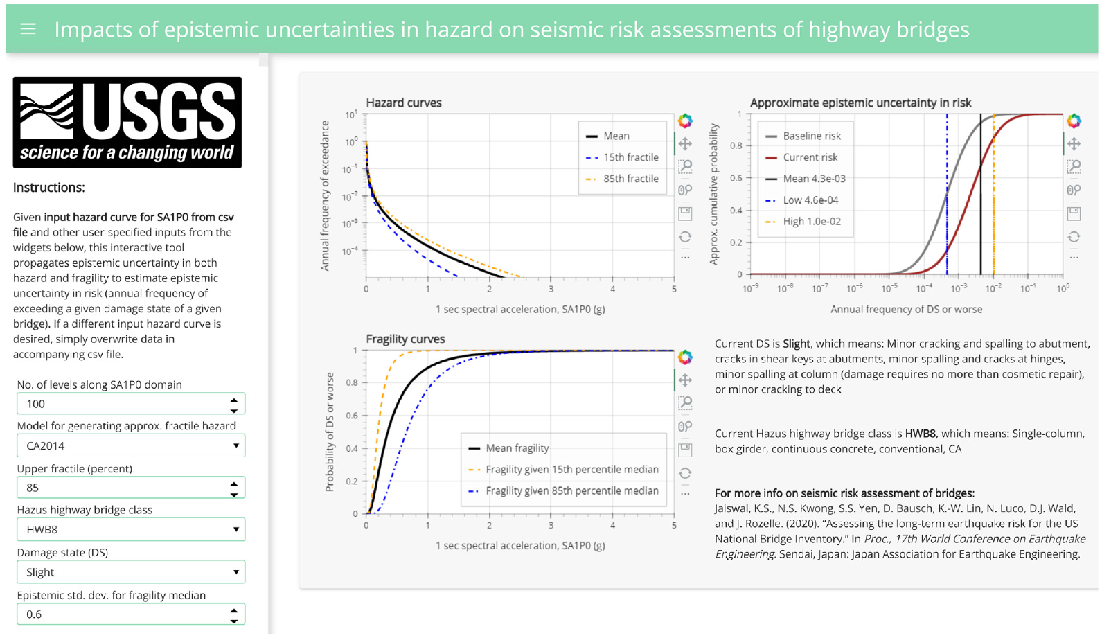
Screenshot of open-source interactive tool for better understanding impacts from epistemic uncertainties in hazard when assessing seismic risks to highway bridges (Kwong and Jaiswal, 2023).

Conclusion

This article aims to help end-users of USGS NSHMs better understand epistemic uncertainties associated with the forecasted earthquake hazard at any given location and shed some light on how such information can potentially be used for hazard and risk applications. Consequently, this article focused on various downstream applications of the epistemic uncertainties in hazard after they have already been quantified or reported. First, we used individual logic tree branch hazard curves from two updates of the USGS NSHM (2014 for California and 2021 for Hawaii) to explicitly illustrate fractile hazard curves and clarify key ideas. Then, we characterized the nature of such epistemic uncertainties in the hazard, resulting in models for readily generating approximate fractile hazard curves in California and Hawaii. Next, we provided specific example uses of fractile hazard curves, for both hazard and risk contexts. Finally, we developed an open-source interactive tool to enable a broad range of users to independently examine and potentially start using epistemic uncertainties for their respective applications.

This investigation led to the following conclusions:

The epistemic uncertainty in hazard is generally larger for Hawaii than for California, except for 0.2-s spectral accelerations at very small AFEs (very long return periods).

The epistemic uncertainty in hazard can be reasonably approximated with a lognormal distribution in most of the cases considered, with the approximation sometimes less reasonable for very small AFEs (very long return periods).

In general, the epistemic uncertainty in hazard is approximately constant at very small intensity levels and increases with increasing intensity level, but the precise relation varies with both location and type of intensity measure.

Approximate fractile hazard curves from the newly developed models agree reasonably well with the more exact fractile hazard curves for most of the cases considered, with poorer agreement for smaller AFEs.

In general, the correlation between epistemic uncertainty in hazard at two different intensity measure levels varies with both location and type of intensity measure.

Example uses of fractile hazard curves include but are not limited to the following:

(a) Determining confidence in UHGMs.

(b) Visualizing epistemic uncertainty in UHGM maps.

(d) Evaluating buildings that were designed from mean hazard.

(e) Propagating epistemic uncertainties in site-specific seismic risk assessments of bridges.

(f) Comparing epistemic uncertainties in hazard against other types of uncertainties in regional seismic risk assessments of pipelines.

Footnotes

Appendix 1

To make the risk-related examples in this article self-contained and maximally accessible to a variety of end-users of the USGS NSHMs, we summarize salient risk-related concepts in this Appendix 1.

The annual frequency of exceeding a given damage state (e.g. collapse of a building, slight damage of a bridge, leak of a pipeline), λ DS , can be computed from the following (e.g. Baker et al., 2021; McGuire, 2004):

(6)

λ DS = ∫ 0 ∞ P ( DS ≥ ds ∣ IM = im ) · | d λ IM ( im ) |

where P ( DS ≥ ds ∣ IM = im ) denotes the conditional probability of exceeding the damage state for a given intensity measure level (i.e. the fragility curve), and λ IM ( im ) denotes the hazard curve. In practice, the fragility curve is commonly modeled using a lognormal CDF with a median of θ DS and a logarithmic standard deviation of β DS ; although the logarithmic standard deviation is commonly assumed to be constant across multiple damage states (Federal Emergency Management Agency (FEMA), 2022), we retain the subscript DS herein for generality. Consequently, Equation 6 may be expressed alternatively as:

(7)

λ DS = ∫ 0 ∞ Φ ( ln [ im θ DS ] β DS ) · | d λ IM ( im ) | = ∫ 0 ∞ λ IM ( im ) · ϕ ( ln [ im θ DS ] β DS ) · d im

where the second line is readily derived from integration by parts, Φ ( · ) denotes the standard normal CDF, and ϕ ( · ) denotes the standard normal probability density function (PDF).

By specifying λ IM ( im ) , λ DS , and β DS in Equation 7 to be, respectively, λ IM * ( im ) , λ DS * , and β DS * , Equation 7 can be iteratively solved to determine the risk-targeted median, θ DS * . Moreover, by specifying P ( DS ≥ ds ∣ IM = im ) to be P * ( DS ≥ ds ∣ IM = im ) , the RTGM value can be determined by solving the following equation:

(8)

P * ( DS ≥ ds ∣ IM = im ) = Φ ( ln [ RTGM θ DS * ] β DS * )

Like the hazard curve, λ IM ( im ) , the fragility curve, P ( DS ≥ ds ∣ IM = im ) , also contains epistemic uncertainty. One common approach to modeling this epistemic uncertainty is to use the double-lognormal fragility model, in which the fragility curve still follows a lognormal CDF with a known aleatory logarithmic standard deviation, β R , but the fragility median now also follows its own lognormal distribution (Kennedy et al., 1980; Shinozuka et al., 2000). With this formulation, the epistemic mean fragility curve becomes the following (Baker et al., 2021):

(9)

E [ P ( DS ≥ ds ∣ IM = im ) ] = ∫ 0 ∞ Φ ( ln [ im s ] β R ) · f θ ( s ) · d s

where f θ ( s ) denotes the lognormal PDF of the fragility median, θ DS , with a median of s and a logarithmic standard deviation of β U . Furthermore, the previous notation of β DS in Equation 7 is now replaced by the notation β R in Equation 9 to explicitly distinguish this aleatory variability from the epistemic uncertainty β U . In practice, the formulation in Equation 9 implies that the mean fragility curve follows a lognormal CDF, with a median of θ DS and an inflated logarithmic standard deviation of β total = β R 2 + β U 2 .

Acknowledgements

The authors thank Kevin Milner for providing the individual branch hazard curves from OpenSHA that formed the basis of the fractile hazard curves in California. They thank Allison Shumway for providing the individual branch hazard curves from nshmp-haz that formed the basis of the fractile hazard curves in Hawaii. This research has benefited from guidance from members of the NSHM steering committee as well as discussions with the NSHM Project Team. They thank two anonymous reviewers, the journal Editor, Max Schneider, Brian Shiro, and Janet Carter for providing helpful comments that improved the manuscript. Finally, they also thank Heather Hunsinger and Jason Altekruse for providing feedback that improved the accompanying software release. Any use of trade, firm, or product names is for descriptive purposes only and does not imply endorsement by the US Government.

Declaration of conflicting interests

The author(s) declared no potential conflicts of interest with respect to the research, authorship, and/or publication of this article.

Funding

The author(s) received no financial support for the research, authorship, and/or publication of this article.

ORCID iD

N. Simon Kwong

Notes

References

Abrahamson

(2006) Seismic hazard assessment: Problems with current practice and future developments. In: Proceedings of the 1st European conference on earthquake engineering and seismology, Geneva: Swiss Society for Earthquake Engineering and Structural Dynamics (SGEB), 3–8 September, pp. 8590–8606.

Abrahamson

Bommer

(2005) Probability and uncertainty in seismic hazard analysis. Earthquake Spectra 21(2): 603–607.

Al Atik

Youngs

(2014) Epistemic uncertainty for NGA-West2 models. Earthquake Spectra 30(3): 1301–1318.

Allen

Wald

(2009) On the use of high-resolution topographic data as a proxy for seismic site conditions (V_S30). Bulletin of the Seismological Society of America 99(2A): 935–943.

Altekruse

Powers

(2021) Data Release for PGV Data for the 2018 National Seismic Hazard Model for the Conterminous United States (US Geological Survey (USGS) data release). Reston, VA: USGS.

Anagnos

Kiremidjian

(1988) A review of earthquake occurrence models for seismic hazard analysis. Probabilistic Engineering Mechanics 3(1): 3–11.

Anderson

(2018) Quantifying the epistemic uncertainty in the probabilistic seismic hazard from two major faults in western Nevada. Earthquake Spectra 34(2): 549–568.

Anderson

Brune

(1999) Probabilistic seismic hazard analysis without the ergodic assumption. Seismological Research Letters 70(1): 19–28.

Ang

AH-S

Tang

(2007) Probability Concepts in Engineering: Emphasis on Applications to Civil and Environmental Engineering. 2nd ed. Hoboken, NJ: Wiley, 432 pp.

10.

Atkinson

Bommer

Abrahamson

(2014) Alternative approaches to modeling epistemic uncertainty in ground motions in probabilistic seismic-hazard analysis. Seismological Research Letters 85(6): 1141–1144.

11.

Baker

Bradley

Stafford

(2021) Seismic Hazard and Risk Analysis. 1st ed. Cambridge: Cambridge University Press, 582 pp.

12.

Bommer

Scherbaum

Bungum

Cotton

Sabetta

Abrahamson

(2005) On the use of logic trees for ground-motion prediction equations in seismic-hazard analysis. Bulletin of the Seismological Society of America 95(2): 377–389.

13.

Boyd

(2012) Including foreshocks and aftershocks in time-independent probabilistic seismic-hazard analyses. Bulletin of the Seismological Society of America 102(3): 909–917.

14.

Bradley

(2009) Seismic hazard epistemic uncertainty in the San Francisco Bay Area and its role in performance-based assessment. Earthquake Spectra 25(4): 733–753.

15.

Budnitz

Apostolakis

Boore

Cluff

Coppersmith

Cornell

Morris

(1997) Recommendations for Probabilistic Seismic Hazard Analysis: Guidance on Uncertainty and Use of Experts (NUREG/CR-6372), vol. 1. Washington, DC: US Nuclear Regulatory Commission, 280 pp.

16.

Cao

Petersen

Frankel

(2005) Model uncertainties of the 2002 update of California seismic hazard maps. Bulletin of the Seismological Society of America 95(6): 2040–2057.

17.

Cramer

(2001) A seismic hazard uncertainty analysis for the New Madrid seismic zone. Engineering Geology 62(1–3): 251–266.

18.

Der Kiureghian

(2005) Non-ergodicity and PEER’s framework formula. Earthquake Engineering & Structural Dynamics 34(13): 1643–1652.

19.

Der Kiureghian

Ditlevsen

(2009) Aleatory or epistemic? Does it matter? Structural Safety 31(2): 105–112.

20.

Federal Emergency Management Agency (FEMA) (2022) Hazus Earthquake Model Technical Manual (Hazus 5.1). Washington, DC: FEMA, 467 pp.

21.

Field

Arrowsmith

Biasi

Bird

Dawson

Felzer

Jackson

Johnson

Jordan

Madden

Michael

Milner

Page

Parsons

Powers

Shaw

Thatcher

Weldon

II Zeng

(2014) Uniform California earthquake rupture forecast, version 3 (UCERF3)—The time-independent model. Bulletin of the Seismological Society of America 104(3): 1122–1180.

22.

Field

Milner

Porter

(2020) Assessing the value of removing earthquake-hazard-related epistemic uncertainties, exemplified using average annual loss in California. Earthquake Spectra 36(4): 1912–1929.

23.

Frankel

Mueller

Barnhard

Perkins

Leyendecker

Dickman

Hanson

Hopper

(1996) National seismic-hazard maps: Documentation June 1996. US Geological Survey (USGS) open-file report 96-532, June 1996, 110 pp. Reston, VA: USGS.

24.

Frankel

Petersen

Mueller

Haller

Wheeler

Leyendecker

Wesson

Harmsen

Cramer

Perkins

Rukstales

(2002) Documentation for the 2002 update of the National Seismic Hazard Maps. US Geological Survey (USGS) open-file report 02-420, 33 pp. Reston, VA: USGS.

25.

Hamburger

Bonneville

Crouse

Dolan

Enfield

Furr

Hanson

Harris

Heintz

Holmes

Hooper

Kircher

Luco

McCabe

Pekelnicky

Siu

Rezaeian

Schneider

Stewart

Sattar

Tong

Yuan

(2017) Development of the next generation of seismic design value maps for the 2020 NEHRP provisions. BSSC project 17 final report, National Institute of Building Sciences, Washington, DC, 30 September 2022, 143 pp. Available at: https://www.nibs.org/reports/bssc-project-17-final-report-development-next-generation-seismic-design-value-maps-2020

26.

Haselton

Baker

Stewart

Whittaker

Luco

Fry

Hamburger

Zimmerman

Hooper

Charney

Pekelnicky

(2017) Response history analysis for the design of new buildings in the NEHRP provisions and ASCE/SEI 7 standard: Part I—Overview and specification of ground motions. Earthquake Spectra 33(2): 373–395.

27.

Jaiswal

Kwong

Yen

Bausch

Lin

K-W

Luco

Wald

Rozelle

(2020) Assessing the long-term earthquake risk for the US National Bridge Inventory. In: Proceedings of the 17th world conference on earthquake engineering, Sendai, Japan: Japan Association for Earthquake Engineering, 13–18 September, 9 pp.

28.

Kennedy

Cornell

Campbell

Kaplan

Perla

(1980) Probabilistic seismic safety study of an existing nuclear power plant. Nuclear Engineering and Design 59(2): 315–338.

29.

Kulkarni

Youngs

Coppersmith

(1984) Assessment of confidence intervals for results of seismic hazard analysis. In: Proceedings of the 8th world conference on earthquake engineering, San Francisco, CA: Earthquake Engineering Research Institute (EERI), 21–28 July, pp. 263–270.

30.

Kwong

N.S.

Jaiswal

K.S.

(2023) brit: Bridge risk interactive tool for exploring impacts from epistemic uncertainties in USGS NSHMs. U.S. Geological Survey software release. DOI: 10.5066/P9N5QTIN.

31.

Kwong

Jaiswal

Baker

Luco

Ludwig

Stephens

(2022) Earthquake risk of gas pipelines in the conterminous United States and its sources of uncertainty. ASCE-ASME Journal of Risk and Uncertainty in Engineering Systems, Part A: Civil Engineering 8(1): 04021081.

32.

Lee

Graf

(2018) Characterizing the epistemic uncertainty in the USGS 2014 National Seismic Hazard Mapping Project (NSHMP). Bulletin of the Seismological Society of America 108(3A): 1465–1480.

33.

Lee

Graf

Thiel

Jr Hu

Ellis

(2022) Seismic risk assessments for real estate portfolios: Impact of engineering investigation on quality of seismic risk studies. Earthquake Spectra 38(1): 726–755.

34.

Luco

Ellingwood

Hamburger

Hooper

Kimball

Kircher

(2007) Risk-targeted versus current seismic design maps for the conterminous United States. In: Proceedings of the Structural Engineers Association of California (SEAOC) 2007 convention, Squaw Creek, CA, 26–29 September, 13 pp. Sacramento, CA: SEAOC.

35.

McGuire

(1977) Effects of uncertainty in seismicity on estimates of seismic hazard for the east coast of the United States. Bulletin of the Seismological Society of America 67(3): 827–848.

36.

McGuire

(2004) Seismic Hazard and Risk Analysis. Oakland, CA: Earthquake Engineering Research Institute (EERI), 240 pp.

37.

McGuire

Cornell

Toro

(2005) The case for using mean seismic hazard. Earthquake Spectra 21(3): 879–886.

38.

Miller

Baker

(2015) Ground-motion intensity and damage map selection for probabilistic infrastructure network risk assessment using optimization. Earthquake Engineering & Structural Dynamics 44(7): 1139–1156.

39.

Moehle

Deierlein

(2004) A framework methodology for performance-based earthquake engineering. In: Proceedings of the 13th world conference on earthquake engineering, Vancouver, BC, Canada: International Association for Earthquake Engineering, 1–6 August, 13 pp.

40.

Musson

(2012) On the nature of logic trees in probabilistic seismic hazard assessment. Earthquake Spectra 28(3): 1291–1296.

41.

Nadav-Greenberg

Joslyn

Taing

(2008) The effect of uncertainty visualizations on decision making in weather forecasting. Journal of Cognitive Engineering and Decision Making 2(1): 24–47.

42.

National Academies of Sciences, Engineering, and Medicine (NASEM) (2019) Reproducibility and Replicability in Science. Washington, DC: The National Academies Press, 234 pp.

43.

National Research Council (NRC) (1988) Probabilistic Seismic Hazard Analysis. Washington, DC: The National Academies Press, 111 pp.

44.

NSHM Steering Committee (2020) National Seismic Hazard Model project steering committee. Meeting report, US Geological Survey (USGS), Golden, CO, 16 January.

45.

Petersen

Frankel

Harmsen

Mueller

Haller

Wheeler

Wesson

Zeng

Boyd

Perkins

Luco

Field

Wills

Rukstales

(2008) Documentation for the 2008 update of the United States national seismic hazard maps. US Geological Survey (USGS) open-file report 2008-1128, May 2008 61 pp. Reston, VA: USGS.

46.

Petersen

Moschetti

Powers

Mueller

Haller

Frankel

Zeng

Rezaeian

Harmsen

Boyd

Field

Chen

Rukstales

Luco

Wheeler

Williams

Olsen

(2015) The 2014 United States national seismic hazard model. Earthquake Spectra 31(S1): S1–S30.

47.

Petersen

Shumway

Powers

Moschetti

Llenos

Michael

Mueller

Frankel

Rezaeian

Rukstales

McNamara

Okubo

Zeng

Jaiswal

Ahdi

Altekruse

Shiro

(2022) 2021 US National seismic hazard model for the State of Hawaii. Earthquake Spectra 38(2): 865–916.

48.

Petersen

Shumway

Powers

Mueller

Moschetti

Frankel

Rezaeian

McNamara

Luco

Boyd

Rukstales

Jaiswal

Thompson

Hoover

Clayton

Field

Zeng

(2020) The 2018 update of the US National Seismic Hazard Model: Overview of model and implications. Earthquake Spectra 36(1): 5–41.

49.

Powers

Clayton

Altekruse

(2022) nshmp-haz: National Seismic Hazard Model Project Hazard Applications and Web Services (US Geological Survey (USGS) software release). Reston, VA: USGS.

50.

Retchless

Brewer

(2016) Guidance for representing uncertainty on global temperature change maps. International Journal of Climatology 36(3): 1143–1159.

51.

Rezaeian

Petersen

Moschetti

Powers

Harmsen

Frankel

(2014) Implementation of NGA-West2 ground motion models in the 2014 US National Seismic Hazard Maps. Earthquake Spectra 30(3): 1319–1333.

52.

Schneider

McDowell

Guttorp

Steel

Fleischhut

(2022) Effective uncertainty visualization for aftershock forecast maps. Natural Hazards and Earth System Sciences 22(4): 1499–1518.

53.

Shinozuka

Feng

Lee

Naganuma

(2000) Statistical analysis of fragility curves. Journal of Engineering Mechanics: ASCE 126(12): 1224–1231.

54.

Shumway

Clayton

Rukstales

(2021) Data Release for Additional Period and Site Class Data for the 2018 National Seismic Hazard Model for the Conterminous United States (version 1.2, May; US Geological Survey (USGS) data release). Reston, VA: USGS.

55.

Soleimani

Davidson

Davis

O’Rourke

Nozick

(2021) Multihazard scenarios for regional seismic risk assessment of spatially distributed infrastructure. Journal of Infrastructure Systems 27(1): 4021001.

56.

Stepp

Wong

Whitney

Quittmeyer

Abrahamson

Toro

Young

Coppersmith

Savy

Sullivan

(2001) Probabilistic seismic hazard analyses for ground motions and fault displacement at Yucca Mountain, Nevada. Earthquake Spectra 17(1): 113–151.

57.

Stevens

J-LR

Rudiger

Bednar

(2015) HoloViews: Building complex visualizations easily for reproducible science. In: Proceedings of the 14th Python in science conference, Austin, TX: SciPy, 6–12 July, pp. 59–66.

58.

Working Group on California Earthquake Probabilities (2003) Earthquake probabilities in the San Francisco Bay region: 2002-2031. US Geological Survey (USGS) open-file report 2003-214, May 2003, 235 pp. Reston, VA: USGS.

59.

Zimmerman

Baker

Hooper

Bono

Haselton

Engel

Hamburger

Celikbas

Jalalian

(2017) Response history analysis for the design of new buildings in the NEHRP provisions and ASCE/SEI 7 standard: Part III —Example applications illustrating the recommended methodology. Earthquake Spectra 33(2): 419–447.

Uses of epistemic uncertainties in the USGS National Seismic Hazard Models

Abstract

Keywords

Introduction

Epistemic uncertainties in USGS NSHMs

2014 NSHM for California

2021 NSHM for Hawaii

Characterizing epistemic uncertainty in the hazard

Uses of fractile hazard curves

Hazard example 1

Hazard example 2

Hazard example 3

Risk example 1

Risk example 2

Risk example 3

Other potential uses of epistemic uncertainty in the hazard

Conclusion

Footnotes

Appendix 1

Acknowledgements

Declaration of conflicting interests

Funding

ORCID iD

Notes

References