Sage Journals: Discover world-class research

Abstract

The ability to think abstractly and reason by analogy is a prerequisite to rapidly adapt to new conditions, tackle newly encountered problems by decomposing them, and synthesize knowledge to solve problems comprehensively. We present TransCoder, a method for solving abstract problems based on neural program synthesis, and conduct a comprehensive analysis of decisions made by the generative module of the proposed architecture. At the core of TransCoder is a typed domain-specific language, designed to facilitate feature engineering and abstract reasoning. In training, we use the programs that failed to solve tasks to generate new tasks and gather them in a synthetic dataset. As each synthetic task created in this way has a known associated program (solution), the model is trained on them in supervised mode. Solutions are represented in a transparent programmatic form, which can be inspected and verified. We demonstrate TransCoder’s performance using the Abstract Reasoning Corpus dataset, for which our framework generates tens of thousands of synthetic problems with corresponding solutions and facilitates systematic progress in learning.

Keywords

neurosymbolic systems program synthesis abstract reasoning

1. Introduction

Abstract reasoning tasks have a long-standing history in artificial intelligence, as epitomized with Bongard’s problems (Bongard, 1967), Hofstadter’s analogies (Hofstadter, 1995), and more recently the Abstract Reasoning Corpus (ARC; Chollet, 2019; Figure 1). They reach beyond the input–output mapping tasks typical for contemporary machine learning (e.g., classification and regression) and thus pose several nontrivial challenges. The suits of such tasks tend to be very diverse, each engaging a different “conceptual apparatus” and thus requiring a bespoke solution strategy. This, in turn, implies the necessity of devising sophisticated features that are highly task-specific and need to be “invented on the spot,” such as the presence/absence of previously unseen objects in the visual input, or the number of tokens in a sequence, or a specific pattern thereof. Another challenge is the staged nature of reasoning, which often needs to comprise multiple steps of inference, thus requiring some notion of working memory for storing and manipulating diverse concepts.

Figure 1.

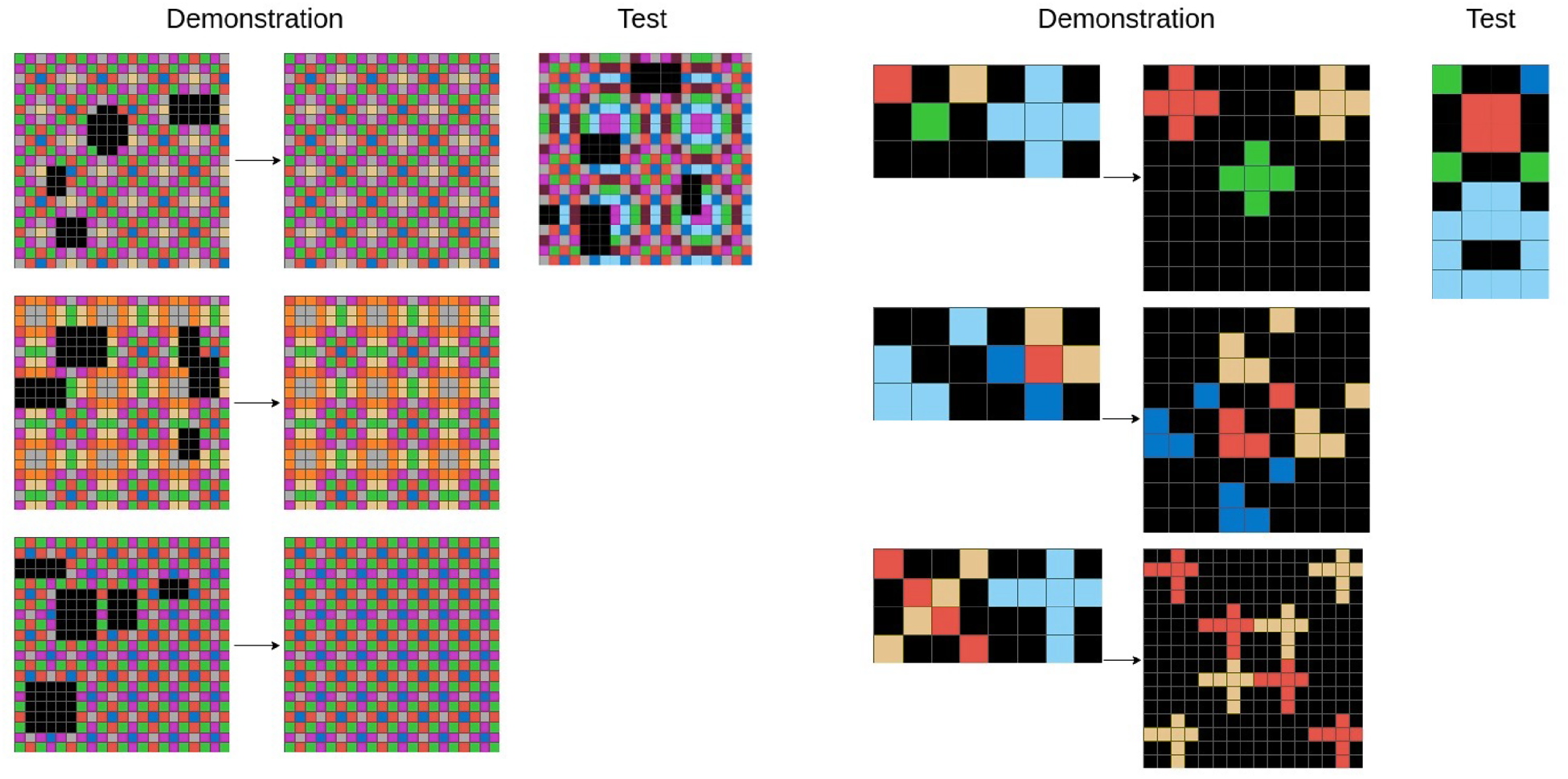
Examples from the Abstract Reasoning Corpus dataset.

These and other characteristics of abstract reasoning tasks become particularly challenging when one attempts to learn to solve them, rather than manually devising a complete architecture of a working solver. Given the diversity of the tasks to be faced, one cannot rely on predefined representations and concepts, and often not even on preset solving strategies, and it becomes essential to allow the learner to construct them on the fly and, in particular, to learn what to construct given the context of the given task.

In the past, abstract reasoning tasks have been most often approached with algorithms relying exclusively on symbolic representations, typically involving some form of principled logic-based inference. While this can be successful for problems posed “natively” in symbolic terms (e.g., Hofstadter, 1995), challenges start to mount up when a symbolic representation needs to be inferred from a low-level, for example, visual, representation (Bongard, 1967; Chollet, 2019). The recent advances in deep learning and increasing possibilities of their hybridization with symbolic reasoning (see Section 4) opened the door to architectures that combine “subsymbolic” processing required to perceive the task with sound symbolic inference.

Addressing the above challenges requires a flexible, expressive, structural, and compositional formalism that permits the learner to experiment with alternative representations and features of the task, combine and validate them, and so learn successful problem-solving strategies. While devising completely new mechanisms for this purpose is arguably possible, it is natural in our opinion to reach the realm of programming languages, and to pose the problem of solving abstract reasoning problems as a program synthesis task. In this formulation, the solver is an intelligent, reactive agent that perceives the task and attempts to synthesize a program in a bespoke domain-specific language (DSL) which, once executed, produces the solution to the task.

This study is based on these premises and introduces TransCoder, a neurosymbolic architecture that relies on both neural and symbolic perception of the problem and involves programmatic representations to detect and capture relevant patterns in low-level representations of the task, infer higher-order structures from them, and encode the transformations required to solve the task. TransCoder is designed to handle the tasks from the ARC (Chollet, 2019), a popular benchmark that epitomizes the above-mentioned challenges. Our main contributions include (i) the original neurosymbolic architecture that synthesizes programs that are syntactically correct by construction, (ii) the “learning from mistakes” paradigm for generating synthetic tasks of adequate difficulty to provide TransCoder with a learning gradient, (iii) an advanced perception mechanism to reason about small-size rasters of variable size, and (iv) an empirical assessment on the ARC suite. This paper extends the preliminary findings summarized in the conference paper (Bednarek & Krawiec, 2024) and uses an improved version of TransCoder architecture.

2. Abstract Reasoning Corpus (ARC)

ARC (Chollet, 2019) is a collection of 800 tasks of a visual nature, partitioned into 400 training tasks and 400 testing tasks.¹ Each task comprises a set of input–output pairs that exemplify a mapping/rule to be discovered. That set is divided into demonstrations and tests. The demonstration set consists of three to six such pairs, while the test set typically contains a single pair. The solver has full access only to demonstrations; for tests, it can observe only the input parts (Figure 1). The test set acts as an independent verification mechanism for evaluating the solutions generated by the solver. Essentially, the solver is challenged to extract the inherent problem definition from demonstrations and subsequently apply this learned knowledge to generate solutions for the inputs in tests. This distinction between the roles of the demonstrations and tests emphasizes the importance of generalization and the ability of the solver to extrapolate beyond the provided examples.

The inputs and outputs in a pair are raster images. Images are usually small (at most $30 \times 30$ pixels), and each pixel can assume one of 10 color values, represented as a categorical variable (there is no implicit ordering of colors).

For each ARC task, there exists at least one processing rule (unknown to the solver) that maps the input raster of each demonstration to the corresponding output raster. The solver is expected to infer² such a rule from the demonstrations and apply it to the test input rasters to produce the corresponding outputs. The output is then submitted to the oracle, which, based on the knowledge of the true/desired outputs, returns a binary response informing about the correctness/incorrectness of the solution.

The ARC collection is extremely heterogeneous in difficulty and nature, featuring tasks that range from simple pixel-wise image processing (e.g., re-coloring of objects), to mirroring of the parts of the image, to combinatorial aspects (e.g., counting objects), to intuitive physics (e.g., an input raster to be interpreted as a snapshot of moving objects and the corresponding output presenting the next state). In quite many tasks, the black color should be interpreted as the background on which objects are presented; however, there are also tasks with rasters filled with “mosaics” of pixels, with no clear foreground–background separation (see, e.g., the left example in Figure 1). Raster sizes can vary between demonstrations, and between the inputs and outputs; in some tasks, it is the size of the output raster that conveys the response to the input. Because of these and other characteristics, ARC is widely considered extremely hard: in the Kaggle contest accompanying the publication of this benchmark,³ which closed on May 28, 2020, the best contestant entry algorithm achieved an error rate of 0.794, that is, solved approximately 20% of the tasks from the (unpublished) evaluation set, and most entries relied on a computationally intensive search of possible input–output mappings. Section 4 reviews selected ARC solvers proposed to date.

3. The Proposed Approach

The broad scope of visual features, object properties, alternative interpretations of images, and inference mechanisms required to solve ARC tasks suggests that devising a successful solver requires at least some degree of symbolic processing. Among others, objects in ARC rasters tend to be small and “crisp,” so that even a single-pixel difference between them matters (not mentioning the fact that some tasks feature single-pixel objects). The conventional convolution-based perception typical for contemporary deep learning models is not sufficient to capture this level of detail, also because they are prepared to process categorical, unordered colors. Moreover, such precision is required not only in perception, but also when producing output rasters to match those in demonstrations or generate the response to the test image.

It is also clear that reasoning conducted by the solver needs to be compositional; for instance, in some tasks, objects must be first delineated from the background and then counted, while in others objects need to be first counted, and only then the foreground–background distinction becomes possible. It is thus essential to equip the solver with the capacity to rearrange the inference steps in an (almost) arbitrary fashion.

Following the motivations outlined in Section 1, the above observation is a strong argument for representing the candidate solutions as programs and forms our main motivation for founding TransCoder on program synthesis, where the solver can express a candidate solution to the task as a program in a DSL, a bespoke programming language designed to handle the relevant entities. Because (i) the candidate programs are to be generated in response to the content of the (highly visual) task, and (ii) it is desirable to make our architecture efficiently trainable with a gradient to the greatest degree possible, it becomes natural to control the synthesis using a neural model. TransCoder is thus a neurosymbolic system that comprises the following components (Figure 2):

Perception: encodes demonstration input–output pairs into latent representations $z_{i}$ of fixed dimensionality, capturing inter-example relationships, where $i$ points to the representation of the $i$ -th demonstration.

Solver: aggregates latent representations $z_{i}$ from the Perception module to a problem latent space $Z$ and samples a latent program representation $z \sim Z$ .

Program Generator (Generator for short): based on the latent program representation $z$ and additional information detailed in Section 3.3, constructs an Abstract Syntax Tree (AST) of the synthesized program $p$ .

Program Interpreter (Interpreter for short): executes $p$ on input rasters to produce the corresponding output rasters, which can then be compared with the expected output rasters.

In training, the Interpreter applies

p

independently to each of the input rasters of demonstrations and returns the predicted output rasters, which are then confronted with the true output rasters using a loss function. In testing,

p

is applied to the test raster, and the resulting raster is submitted to the oracle that determines its correctness.

Figure 2.

The overall architecture of TransCoder comprises Perception, Solver, and Program Generator. The former two are purely neural, while the Generator combines symbolic processing and information from the neural model. The Generator relies on symbolic working memory (Workspace), which maintains both entities specific to individual demonstrations (local) as well as those common for all demonstrations and predefined concepts (global).

We detail the components of TransCoder in the following sections. For technical details, see Appendix A.

3.1. The Perception Module

The Perception module comprises the raster encoder and the demonstration encoder.

As argued at the beginning of this section (and verified in our preliminary studies), typical convolutional layers are insufficient for capturing the information that is essential in ARC tasks. Therefore, we abandon purely convolutional processing in favor of encoding rasters as one-dimensional sequences of tokens that convey information about pixels. Prior to the sequential processing block, the data undergoes a preprocessing with two 2D convolutional layers. The layers preserve the spatial dimensions of the input tensor, ensuring that both height and width remain unchanged, which is essential due to extremely small rasters in the dataset. The information about the raster size itself, often crucial for solving the task, is also conveyed by the length of the sequence.

Our raster encoder is based on an attention module that allows processing rasters of different sizes, which is required when solving ARC tasks (see, e.g., the task shown in Figure 2). Each pixel resulting from the last convolutional layer gives rise to a separate token, tagged with the color and $(x, y)$ coordinates, the latter acting as input to a positional embedding layer, architecturally similar to those employed in transformer models Vaswani et al. (2017), but adapted for a 2D spatial context. This embedding strategy allows the model to explicitly incorporate spatial information into its representation of the input data. The resulting tokens are flattened into a one-dimensional sequence (see the left part of Figure 3), which is then processed by a series of eight self-attention blocks. Subsequently, a global average pooling operation reduces the final sequence to a single, fixed-size vector, yielding a compact representation of the raster. These raster representations are then passed to the demonstration encoder.

Figure 3.

The autoencoder architecture used to pre-train the raster encoder in perception. Left: the encoder (used in TransCoder after pre-training). Right: the decoder (used only in pre-training and then discarded).

The raster encoder can be trained alongside the other TransCoder components; however, this turned out to be computationally inefficient. More importantly, when training the entire architecture end-to-end, it is hard to determine the component that should be blamed for the failure to deliver the correct answer. For these reasons, we pre-train the raster encoder within an autoencoder architecture, where the encoder is combined with a compatible decoder that can reproduce varying-length sequences of pixels (and thus the input raster) from a fixed-dimensionality latent. The decoder is shown in the right part of Figure 3 and comprises a sequence of steps that attempt to recover the spatial and color information from the fixed-dimensional latent.

The objective of pre-training is to develop an encoder capable of effectively encapsulating the essential information from the input data in the latent representation. To achieve this, we train the autoencoder in the self-supervision mode, by confronting it with a “fill-in” task. The decoder is tasked with predicting the correct pixel value (pixel color) at a given location, conditioned on the latent representation of the input raster from the encoder. By providing the decoder with the complete set of target pixel positions, the requirement for the decoder to determine the output raster is relaxed (compared to an alternative scenario in which one could require the decoder to restore the entire sequence, i.e., both colors and coordinates). The decoder then concatenates the embeddings of target positions with the reduced raster representation to prevent the encoder from overspecializing on the “fill-in” tasks. As the “query” position representation contains partial raster representation, the encoder is forced to reason in terms of dependencies between pixels and their colors and coordinates, rather than overfitting to specific locations and colors of pixels. The decoder then processes the tokens with a stack of cross-attention blocks. Eventually, a fully connected layer produces per-pixel predictions, which are confronted with the actual pixels from the input sequence using pixel-wise categorical cross-entropy loss on the color variable.

The autoencoder is pre-trained until convergence, using all rasters (inputs, outputs, and tests) collected from the training part of the ARC collection. In this process, we intend to make feature extraction invariant to permutations of colors, while accounting for the black color serving the special role of the background in a large fraction of tasks. To this end, the rasters derived from the ARC are treated as dynamic templates, which are being randomly re-colored on the fly, while preserving the distinctions of colors. This enforces permutation-invariance in the space of colors and improves generalization. As a result of pre-training, the raster encoder used in the experimental part of this study achieves the per-pixel reconstruction accuracy of 99.99% and the per-raster accuracy of 96% on the testing part of the original ARC. The resulting encoder is thus guaranteed to pass on almost the entirety of the information available in the input rasters.

Upon completion of pre-training, the raster encoder is prepended to the demonstration encoder in TransCoder. For each demonstration pair, the demonstration encoder invokes the raster encoder twice, separately for the input and output raster, concatenates the resulting latent vectors, and passes them through a two-layer multilayer perceptron (MLP). This is repeated for all demonstrations, and the output vectors produced by the MLP are chained into a sequence, which is then subject to processing with four consecutive self-attention blocks. The final sequence $z_{i}$ is the representation of the demonstrations.

3.2. Solver

The sequential latent $z_{i}$ produced by the perception task forms a representation of demonstrations of the given ARC task. As the raster encoder has been almost perfectly pre-trained via auto-association (see previous section), we expect this sequence to convey the entirety of information about the content of the task.⁴ However, this does not imply the capacity of solving the task. Therefore, the role of the Solver is to map $z_{i}$ to a latent representation $z$ of the program to be synthesized in the DSL, which is meant to act on the task and solve it.

Technically, the Solver is implemented as a two-layer MLP preceded by averaging over the sequence of $z_{i}$ s. In principle, the resulting latent vector $z$ could be directly passed to the Program Generator (Section 3.5). However, as in most programming languages, in our DSL (detailed in Section 3.4), the relationship between the programs (their syntax) and their input–output behaviors (semantics) is many-to-one, that is, the same semantics can be implemented with more than one program. As a result, a given ARC task can be solved with more than one program, and this very program can be a solution to more than one ARC task.

To account for this many-to-many correspondence, we make the Solver stochastic by following the blueprint of the Variational Autoencoder Kingma and Welling (2022): the last layer of Solver’s MLP does not directly produce $z$ , but parameterizes the normal distribution $Z (z_{μ}, z_{σ})$ with two vectors $z_{μ}$ and $z_{σ}$ and then calculates $z = z_{μ} + z_{σ} N (0, 1)$ where $N (0, 1)$ comes from a random number generator. The resulting latent $z$ is subsequently passed to the Program Generator, accompanied by the additional information about the task harvested from the Workspace.

The variational layer allows the Solver to propose alternative solutions to the same ARC task. Ideally, one would hope $z_{μ}$ to represent the centroid of the set of programs that solve a given task (and thus share in this sense a common semantics), while $z_{σ}$ models the extent of that set in the latent space (i.e., the syntactic variations between those programs). Of course, such ideal convergence is not guaranteed, and the subsequent stages of processing do not rely on its emergence. However, as we found in preliminary experiments, the variational layer improves exploration in training.

The presence of sampling makes TransCoder non-deterministic and brings tangible benefits in training: as we found in preliminary experiments, it significantly improves exploration, helping the method to produce non-trivial programs, and is particularly important for generating synthetic tasks (Section 3.7. If desired, sampling can be disabled at test time, with $z_{μ}$ passed as $z$ , allowing for deterministic replication of TransCoder’s querying. Importantly, even though sampling may lead to different programs in response to the same ARC task, each of those programs has well-defined, deterministic semantics, and will always produce the same output when applied to a given input.

3.3. Workspace

The Workspace is the core symbolic module of TransCoder, which is meant to provide the Program Generator (Section 3.5) with additional information, alongside the latent $z$ resulting from the Solver. It supplies the Generator with two types of symbolic entities, that is, (i) the percepts representing parts of the rasters in demonstrations, and (ii) the elements of the DSL, that is, its instructions and constants. The access to both these types of elements is provided in a unified manner, by embedding them in the same space, which allows them to be retrieved on-demand by the Generator during program synthesis, composed in an arbitrary way (limited only by the syntax of the DSL), and ultimately “tried out” via program execution.

Concerning the access to percepts in the Workspace, we supplement the information provided by the Perception module with selected symbolic percepts inferred independently from the task via direct “symbolic parsing” of images. This supplementation is essential, as many ARC tasks involve qualitative and combinatorial concepts (e.g., counting of objects) that cannot be naturally conveyed by the neural nature of processing and representation provided by the Perception module. We provide two data structures for this purpose:

Workspace Template that holds the abstract placeholders for the entities that appear in all tasks’ demonstrations.

Workspaces that “instantiate” that template with concrete values derived from particular demonstrations.

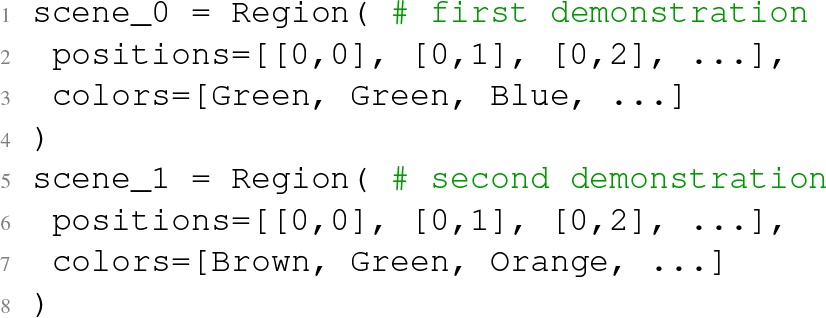
The relation between these two storages can be likened to a dictionary, with the entries in the Workspace Template acting as keys that index specific values (realizations) in the Workspace of a specific demonstration. For instance, the Scene key in the Workspace Template may have a different value in each Workspace. For the task shown in Figure 2, the Workspace Template contains the Scene key, and its values in the first two Workspaces are different, because they feature different sets of colors:

The list of Workspace keys is predefined and includes constants (universal keys shared between all ARC tasks, e.g., zero and one), local invariants (values that repeat within a given task, across all demonstrations, e.g., the set of used colors), and local keys (information specific to a single demonstration pair, e.g., an input Region). For a complete list of available keys, see the Appendix.

The Workspaces require appropriate “neural presentation” for the Generator of DSL programs. For a given task, all keys available in the Workspace Template are first embedded in a Cartesian space, using a learnable embedding similar to those used in conventional deep learning. This representation is context-free, that is, each key is processed independently, and the embedding has in total as many entries as there are unique keys defined in DSL.

Concerning the access to the elements of the DSL, they are also embedded in the same Cartesian space so that the Generator can choose from them, that is, from the DSL instructions and constants from Tables 8 and 7, respectively, alongside the symbolic percepts. In this way, the elements of the DSL are presented to the Generator (on the neural level) in the context of the given task, and, among others, constants (such as “Red”) may have a different embedding depending on the perception result. This is expected to facilitate alternative interpretations of the roles of particular percepts; for instance, while the black pixels should often be interpreted as the background, some tasks are exceptions to this rule.

3.4. The DSL

The DSL we devised for TransCoder is a typed, functional programming language, which allows conveniently representing programs as ASTs. The leaves of ASTs are responsible for fetching input data and constants, inner nodes are occupied by DSL instructions/functions, and the root of the tree produces the return value of the entire program. Each tree node has a well-defined type. The DSL features concrete data types (e.g., Int, Bool, and Region) and generic data types (e.g. List[T]). Tables 1 and 2 present the complete list of, respectively, types and instructions.

Table 1.
The List of Types Available in the Domain-Specific Language (DSL).

Name Description

Arithmetic An abstract type that implements basic arithmetic operations such as addition and subtraction

Bool Logical type

Color Refers to the categorical value of pixels. It can take one of 10 values

Comparable An abstract type that implements basic operations that allow objects to be compared with each other

Int Signed integer (32 bit)

Loc A location consisting of two integers

Connectivity The type of neighborhood used by the FloodFill operation; possible values are n4 and n8

Direction The type of direction used by the Rotate operation; possible values are clockwise (cw) and counterclockwise (cww)

Orientation The type of direction used by the Flip operation; possible values are vertical and horizontal

Region An object representing any list of pixels and their colors

List[T] A generic type representing a list of objects of a compatible type

Pair[T, L] A generic type representing a pair of objects of a compatible type

Name	Description
Arithmetic	An abstract type that implements basic arithmetic operations such as addition and subtraction
Bool	Logical type
Color	Refers to the categorical value of pixels. It can take one of 10 values
Comparable	An abstract type that implements basic operations that allow objects to be compared with each other
Int	Signed integer (32 bit)
Loc	A location consisting of two integers
Connectivity	The type of neighborhood used by the FloodFill operation; possible values are n4 and n8
Direction	The type of direction used by the Rotate operation; possible values are clockwise (cw) and counterclockwise (cww)
Orientation	The type of direction used by the Flip operation; possible values are vertical and horizontal
Region	An object representing any list of pixels and their colors
List[T]	A generic type representing a list of objects of a compatible type
Pair[T, L]	A generic type representing a pair of objects of a compatible type

Table 2.

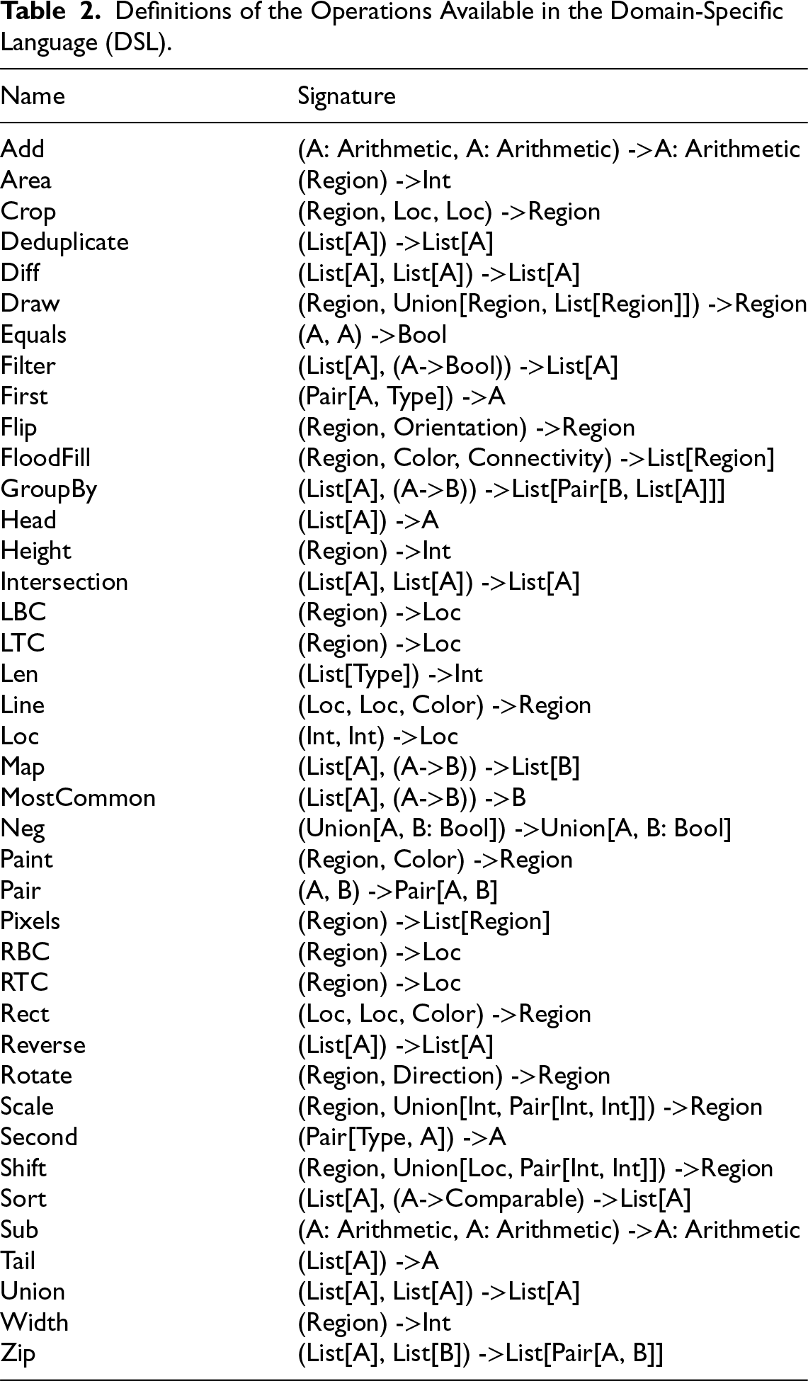
Definitions of the Operations Available in the Domain-Specific Language (DSL).

Name	Signature
Add	(A: Arithmetic, A: Arithmetic) ->A: Arithmetic
Area	(Region) ->Int
Crop	(Region, Loc, Loc) ->Region
Deduplicate	(List[A]) ->List[A]
Diff	(List[A], List[A]) ->List[A]
Draw	(Region, Union[Region, List[Region]]) ->Region
Equals	(A, A) ->Bool
Filter	(List[A], (A->Bool)) ->List[A]
First	(Pair[A, Type]) ->A
Flip	(Region, Orientation) ->Region
FloodFill	(Region, Color, Connectivity) ->List[Region]
GroupBy	(List[A], (A->B)) ->List[Pair[B, List[A]]]
Head	(List[A]) ->A
Height	(Region) ->Int
Intersection	(List[A], List[A]) ->List[A]
LBC	(Region) ->Loc
LTC	(Region) ->Loc
Len	(List[Type]) ->Int
Line	(Loc, Loc, Color) ->Region
Loc	(Int, Int) ->Loc
Map	(List[A], (A->B)) ->List[B]
MostCommon	(List[A], (A->B)) ->B
Neg	(Union[A, B: Bool]) ->Union[A, B: Bool]
Paint	(Region, Color) ->Region
Pair	(A, B) ->Pair[A, B]
Pixels	(Region) ->List[Region]
RBC	(Region) ->Loc
RTC	(Region) ->Loc
Rect	(Loc, Loc, Color) ->Region
Reverse	(List[A]) ->List[A]
Rotate	(Region, Direction) ->Region
Scale	(Region, Union[Int, Pair[Int, Int]]) ->Region
Second	(Pair[Type, A]) ->A
Shift	(Region, Union[Loc, Pair[Int, Int]]) ->Region
Sort	(List[A], (A->Comparable) ->List[A]
Sub	(A: Arithmetic, A: Arithmetic) ->A: Arithmetic
Tail	(List[A]) ->A
Union	(List[A], List[A]) ->List[A]
Width	(Region) ->Int
Zip	(List[A], List[B]) ->List[Pair[A, B]]

Table 3.

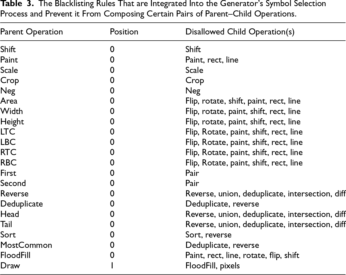
The Blacklisting Rules That are Integrated Into the Generator’s Symbol Selection Process and Prevent it From Composing Certain Pairs of Parent–Child Operations.

Parent Operation	Position	Disallowed Child Operation(s)
Shift	0	Shift
Paint	0	Paint, rect, line
Scale	0	Scale
Crop	0	Crop
Neg	0	Neg
Area	0	Flip, rotate, shift, paint, rect, line
Width	0	Flip, rotate, paint, shift, rect, line
Height	0	Flip, rotate, paint, shift, rect, line
LTC	0	Flip, Rotate, paint, shift, rect, line
LBC	0	Flip, Rotate, paint, shift, rect, line
RTC	0	Flip, Rotate, paint, shift, rect, line
RBC	0	Flip, Rotate, paint, shift, rect, line
First	0	Pair
Second	0	Pair
Reverse	0	Reverse, union, deduplicate, intersection, diff
Deduplicate	0	Deduplicate, reverse
Head	0	Reverse, union, deduplicate, intersection, diff
Tail	0	Reverse, union, deduplicate, intersection, diff
Sort	0	Sort, reverse
MostCommon	0	Deduplicate, reverse
FloodFill	0	Paint, rect, line, rotate, flip, shift
Draw	1	FloodFill, pixels

Within this DSL, a complete program defines a mapping from a set of input values to a corresponding output value of DSL types. Program execution is deterministic, that is, application of a given program to a given input will always produce the same output; however, the variational layer included in the solver (Section 3.2) enables TransCoder to respond with a different program in training and so provide exploration of the program space. Program execution leverages the Workspace for selective retrieval of necessary items using keys. When TransCoder is queried on an ARC problem, the same synthesized DSL program is executed independently for each test Workspace.

The DSL features 40 operations presented in Table 2 (and in Table 8 in more detail). These can be divided into:

data-composing operations (form a more complex data structure from constituents, e.g., Pair and Rect),

property-retrieving operations (fetch elements or extract simple characteristics from data structures, e.g., Width, Area, or Length),

data structure manipulations (e.g., Head of the list, First of a Pair, etc.), arithmetics (Add, Sub, etc.), and

region-specific operations (high-level transformations of drawable objects, e.g. Shift, Paint, and FloodFill).

Our DSL features also higher-order functions, among them Map and Filter, which apply a subprogram to the elements of a compound data structure such as a List. The complete definition of the DSL can be found in the Appendix.

The type system in Table 1 together with the operations in Table 8 implicitly define the grammar of the DSL. We do not present it formally, as the type-parametricity (the generics) makes it context-dependent and quite complex. Crucially, the Program Generator detailed in the subsequent Section 3.5 traverses the combined tree of types and function signatures, and so guarantees the resulting programs to be syntactically correct and thus executable. For similar reasons, we do not attempt to formalize the semantics of the DSL, other than via our implementation of the DSL interpreter, which translates each instruction of the DSL from Table 2 into a snippet of Python code. This implementation and the natural language description in Table 8 provide informal, yet quite precise, denotational semantics of our DSL.

There is a number of arguments in favor of using a bespoke DSL rather than relying on generic languages such as Prolog or/and related approaches such as Inductive Logic Programming (Muggleton & Watanabe, 2014). First, our DSL is already equipped with adequate types for coordinates, regions of connected pixels, and generics (e.g., Pair). This is accompanied by a number of bespoke functions that embody “natural” operations on these data types. These elements of the DSL greatly facilitate learning, especially in the difficult initial phase, which is critical for the successful formation of a model. Secondly, a fair share of ARC puzzles are “operational” in nature, that is, require the input panel to be somehow transformed into the answer panel. It is thus natural to express such transformations as executable sequences (or other control structures) of steps that transform the initial state (as observed in the input panel) into a resulting state, represented by the output panel. Examples include moving objects, connecting pixels with segments, mirroring fragments of the input image, counting objects in the input image, and “expressing” the obtained number in the output raster, and more. Expressing such staged operations in, for example, Prolog, which is declarative rather than imperative, while hypothetically possible, would be quite cumbersome.

Figure 4 shows an example program and the process of its application to an input raster, including the effects of intermediate execution steps.

Figure 4.

Execution process of an example program applied to an input raster (scene). For clarity, we mark the key subprograms with A and B. A adds a constant value of 1 to both coordinates of the upper left corner, that is, Loc(0,0), producing Loc(1,1); this operation exemplifies implicit value casting built-in in our domain-specific language (DSL; alike the “broadcasting” of arrays in Python). B uses the coordinates calculated by A to draw a yellow rectangle. Finally, the program renders the rectangle produced by B on the input raster and returns the so-modified image.

3.5. Program Generator

The Program Generator is a bespoke architecture based on the blueprint of the doubly recurrent neural network (DRNN); see Alvarez-Melis and Jaakkola (2017) for a simple variant of DRNN. The latent $z$ obtained from the Solver (Section 3.2) determines the initial state of this network, which then recursively iterates over the AST nodes of the program being generated.

Before the generation loop, an embedding of each key presented by the Workspace Template is enriched with the information in the latent $z_{j}$ produced by the Perception (Section 3.1) by applying two subsequent cross-attention blocks. This gives the Generator access to precise, symbolic information on demonstration representation, while enabling its “cross-linking” with the presumably less precise, but raster-wide (and thus in this sense global) representation provided by the neural Perception. The resulting vectors form the contextual embeddings $z_{s_{j}}$ of the symbols (values in the Workspace), which are accessed by the Generator in the program generation process described below.

In each iteration, the Generator receives the data on the context, including the current tree size (the number of already generated AST nodes), the depth of the node in the AST, the parent of the current node, and the return type of the node. For the root node, the return type is Region; for other nodes, it is determined recursively by the types of arguments required by DSL functions picked in previous iterations. The Generator is also supplied with the set of symbols available in the Workspaces (including the elements of the DSL), via their embeddings. From this set, the Generator selects only the symbols that meet the requirements regarding the type and the maximum depth of the tree. Then, it applies an attention mechanism to the embedded representations of the selected symbols. The outcome of attention is the symbol to be “plugged” into the AST at the current location. Figure 5 illustrates a few iterations of this process.

Figure 5.

When generating a program, TransCoder uses symbol embeddings available in the Workspace Template. At each step of the breadth-first order generation of a program tree (AST), it computes the probability distribution over all symbols and then selects the one with the highest score. As this process is compliant with DSL’s grammar, some operations may not be available at a given step (the model still calculates the probabilities for such operations, but is not allowed to select from them). The Generator works as long as there are any arguments missing (e.g., in step 1, from the definition of the Paint operation, it follows that two descendants should be generated). Note. AST= Abstract Syntax Tree; DSL=domain-specific language.

By chaining the calls of DSL instructions via type consistency, the generated programs are guaranteed to be syntactically correct. This is an essential advantage of TransCoder, compared to alternative mechanisms based on, for example, language models. In those approaches, programs are stochastically generated sequences of tokens, which need to be checked for syntactic correctness before execution. By providing syntactic correctness by design, the generation mechanism proposed here is more elegant and computationally efficient.

The Generator also determines the hidden state of the DRNN to be passed to each of the to-be-generated children subtrees. This is achieved by merging the current state with a learnable embedding indexed with children’s indices, so that generation in deeper layers of the AST tree is informed about the node’s position in the sequence of parents’ children.

The generation process iterates recursively until the current node requests no children, which terminates the current branch of the AST (but not the others). It is also possible to enforce termination by narrowing down the set of available symbols.

To efficiently utilize computational resources, we adopted the dynamic batching mechanism presented in Bednarek et al. (2018).

3.6. Training

TransCoder can be trained with reinforcement learning (RL) or supervised learning (SL). In RL, the program $p$ synthesized by the Generator is applied to the query raster and returns an output raster, which is then sent to the oracle. The oracle deems it correct or not, and that response determines the value of the reward, which is then used to update the Generator. The reward value is 1 when the oracle’s answer is true for all pairs of demonstration and test; otherwise, the value is 0. Unfortunately, the a priori odds for a generated program to solve the given task are minuscule. As a result, training TransCoder only with RL is usually ineffective and inefficient, especially in the early stages, when the generated programs are almost entirely random: most episodes lead to zero reward and, consequently, no parameter updates. Therefore, based on preliminary experimentation, we abandoned the idea of training TransCoder end-to-end with RL.

The ineffectiveness of RL motivates the SL mode, in which we use the program that solves the given task (target) to guide the Generator. We directly confront the actions of the Generator (i.e., the AST nodes it produces) with the target program node-by-node, and apply a loss function (categorical cross-entropy) that rewards choosing the right symbols at individual nodes and penalizes the incorrect choices. In SL, every prediction produces non-zero gradients, and thus non-zero updates for the model’s parameters (unless the target program has been perfectly generated). We employ the AdamW (Loshchilov & Hutter, 2017) optimizer with default parameter values provided in the TensorFlow (Abadi et al., 2016) library. Additionally, within each outer loop (consecutive training phases culminating in the transition to the exploration phase), the learning rate is adjusted according to the method introduced in Smith (2018) (with five warm-up and 25 decay inner cycles).

The prerequisite for SL is the availability of target programs; as those are not given in the ARC benchmark (in any form, not mentioning our DSL), we devise a method for producing them online during training, presented in Section 3.7. In general, the specific program used as the target will be one of many programs that map the input panels of the task’s demonstrations to the corresponding output panels (see Section 2). Deterministic models cannot realize one-to-many mappings, and the variational layer introduced in Section 3.2 is meant to address this limitation. Upon the ultimate perfect convergence of TransCoder’s training, we would expect the deterministic output of the Solver (corresponding to $z_{μ}$ ) to abstractly represent the common semantic of all programs that solve the presented task, and the variational layer to sample the latents that cause the Generator to produce concrete programs with that very semantics.

3.7. Learning From Mistakes

The programs produced by the Generator are syntactically correct by construction. Therefore, barring the occasional run-time errors (e.g., attempt to retrieve the head of an empty list), a generated program,⁵ applied to an input raster, will always produce some response output raster. By applying such a program $p$ to each of the input rasters $I$ of some task $T$ , we obtain the corresponding list of responses $O$ . We observe that the resulting raster pairs $(x, y) \in I \times O$ form another ARC task $T^{'}$ , to which $p$ is the solution (usually one of possible solutions, to be precise). The resulting pair $(T^{'}, p)$ forms thus a complete example that can be used to train TransCoder in SL mode, as explained in the previous section, where $T^{'}$ is the task to be solved and $p$ is the corresponding target program.

This observation allows us to learn from mistakes: whenever the Generator produces a program $p$ that fails the presented training task $T$ , we pair the inputs with the actual outputs generated by $p$ , add the synthetic task $(T^{'}, p)$ formed in this way to the working collection $S$ of solved tasks, and subsequently use them for SL. Crucially, we expect $T^{'}$ to be on average easier than $T$ , and thus provide the training process with a valuable “learning gradient.” By doing so, we intend to help the model make progress in the early stages of training, when its capabilities fall behind the difficulty of the original ARC tasks.

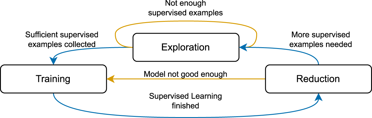
To model the many-to-many relation between tasks and programs, we implement $S$ as a relational database to facilitate the retrieval of all programs (known to date) that solve a given task, and vice versa—the retrieval of all tasks solved by a given program. We disallow duplicates in $S$ .

The top-level learning process starts with $S = \emptyset$ and the working training set $L$ filled with the original ARC tasks, and stages learning into cycles of Exploration, Training, and Reduction phases (Figure 6). As TransCoder spends most of its time iterating between Training and Reduction, this will be referred to as the inner loop of the method; Exploration happens more sparingly, and thus we consider it a part of the outer loop.

Exploration.
The purpose of this phase is to provide synthetic training examples needed in subsequent phases. A random task $T$ is drawn from $L$ , and the Generator is queried on it. If the generated program $p$ solves $T$ , the pair $(T, p)$ is added to $S$ . Otherwise, it is checked whether the response rasters produced by $p$ for $T$ ’s demonstrations meet basic criteria of nontriviality, that is, are non-empty and vary by demonstration. If $T^{'}$ passes this test, $(T^{'}, p)$ is added to the $S$ and $L$ . This continues until enough new tasks have been added to $S$ .
Training.
Training consists of applying SL to a random subset of tasks drawn from $S$ . The execution of this phase ends after iterating $m$ times through all training examples in the drawn subset.
Reduction.
Reduction starts with selecting from $S$ a subset of tasks with known target programs. Then, those tasks are grouped by programs; a group of tasks with the same program forms a category. Next, $n$ categories are drawn at random. Finally, $k$ tasks are drawn for each category. The tasks selected in this way form a working subset $L^{'} \subset L$ .

In the next step, TransCoder is evaluated on $L^{'}$ . For each task $T \in L^{'}$ , if the program produced by the Generator solves $T$ , it is marked as learned and removed from $S$ (if present in $S$ ). Otherwise, $T$ is marked as not learned and added to $S$ (if not present in $S$ ).⁶

Finally, the results for $L^{'}$ are grouped according to the category from which the tasks come, and the average percentage $β$ of solved tasks within each of them is calculated. If $β$ reaches the minimum threshold $β_{min}$ in $n_{s}$ consecutive iterations of the Training stage, we declare stagnation and switch to the Exploration phase, invoking a new iteration of the outer loop; otherwise, we move to the Training phase (i.e., continue iterating in the inner Training-Reduction loop in Figure 6).

Figure 6.
The state diagram of TransCoder’s training, including learning from mistakes.
4. Related Work

TransCoder engages programs, that is, a class of symbolic entities, to process and interpret the input data, and thus bears similarity to several past works on neurosymbolic systems, of which we review only the most prominent ones.

In synthesizing programs in response to input (here: task), TransCoder resembles the Neuro-Symbolic Concept Learner (NSCL; Mao et al., 2019). NSCL was designed to solve Visual Query Answering tasks (Johnson et al., 2016) using object-centric representation and learn to parameterize a semantic parser that translated a natural language query about scene content to a DSL program which, once executed, produced the answer to the question. The system was trained with RL, with a binary reward function that reflected the correctness of the answer provided to the query. Interestingly, NSCL’s DSL was implemented in a differentiable fashion, which allowed it to inform its perception subnetwork in training.

With respect to abstract reasoning, the key characteristic aspect of the ARC suite, a similar “object-centric” approach is taken by Assouel et al. (2022), which operates on a category of ARC tasks. The work relies on strong assumptions about the tasks from the considered category and provides a DSL for manipulating and transforming objects typical of rasters used in those tasks. This formalism allows the authors to generate new unseen tasks, which are subsequently used to train their model, in a fashion similar to TransCoder. However, the proposed approach does not involve program synthesis nor a DSL per se.

The most successful approaches in the ARC 2020 Kaggle challenge often relied on an assembly of various processing techniques, including brute-force search, handcrafting features, manual data labeling, and DSL-guided search. The results of the competition corroborated the awareness of the usefulness of the program synthesis approach with data-tailored DSLs, and resulted in approaches which engaged, among others, descriptive grids and the minimum-description length principle (Ferré, 2021), graph-based representations (Xu et al., 2022), or combining DreamCoder (Ellis et al., 2021) with a search graph (Alford et al., 2021). To a greater or lesser extent, many of those methods also engaged an exhaustive search, which is notably absent in TransCoder.

In using a program synthesizer to produce new tasks, rather than only to solve the presented tasks, TransCoder bears some similarity to the DreamCoder (Ellis et al., 2021). DreamCoder’s training proceeds in cycles comprising wake, dreaming, and abstraction phases, which realize, respectively, solving the original problems, training the model on “replays” of the original problems and on “fantasies” (synthetic problems), and refactorization of the body of synthesized programs. The last phase involves identification of the often-occurring and useful snippets of programs, followed by encapsulating them as new functions in the DSL, which is meant to facilitate “climbing the abstraction ladder.” The DreamCoder was shown to achieve impressive capabilities on a wide corpus of problems, ranging from typical program synthesis to symbolic regression to interpretation of visual scenes. For a thorough review of other systems of this type, the reader is referred to Chaudhuri et al. (2021).

Recent advancements in large language models (LLMs) have led researchers to explore their capabilities in abstract reasoning tasks, notably the ARC and RAVEN (Zhang et al., 2019) benchmarks. An extensive analysis of ARC was conducted in Moskvichev et al. (2023), resulting in a comparison of Kaggle 2020 competition winner methods, GPT 4, and human performances on ConceptARC, a categorized version of the ARC dataset proposed in that study. One of the main findings of this study was humans’ superior capability, compared to all considered algorithmic methods. Extensive research on LLMs applied to ARC tasks and other problems (Mirchandani et al., 2023) has demonstrated significant improvements through prompt engineering techniques in ARC solving, and pointed to the overall capacity of those models as sequence modelers and quite successful pattern extrapolators. These advances have enabled LLMs to surpass the accuracy of many DSL-based methods, achieving accuracy rates of approximately 10% without fine-tuning, and often via zero-shot learning via prompting.

The Perception module draws inspiration from the vision transformer architecture (Dosovitskiy et al., 2020), interleaving self-attention and cross-attention blocks (Vaswani et al., 2017) with reduction blocks (Lin et al., 2014).

5. Experimental Evaluation

In the following experiment, we examine TransCoder’s capacity to provide itself with a “reflexive learning gradient,” meant as a continuous supply of synthetic tasks at the level of difficulty that facilitates further improvement. Therefore, we focus on the dynamics of the learning process.

Setup. To ensure a sufficiently large pool of training examples, each Exploration phase lasts until the set of solved tasks $S$ contains at least 8,192 tasks and 32 unique solutions. During each Training phase, a random subset of 8,192 tasks is sampled without replacement from $S$ . The Training phase comprises $m = 4$ iterations over this sampled subset, with the order of tasks randomized in each iteration. For the Reduction phase, we set the number of categories to be drawn for $L^{'}$ to $n = 512$ , the number $k$ of tasks to be drawn from each category to 16, the solving threshold $β_{min}$ to 30%, and the number of stagnation iterations $n_{s} = 3$ . Additionally, if the model achieves $β \geq 80 %$ , the reduction phase stops, and another Training phase begins. The programs synthesized by the Generator are limited to 64 nodes, a maximum depth of 8, and at most two nestings of higher-order functions. Each invocation of a nested higher-order function is considered a separate program and is also required to meet the above constraints.

To enhance the efficiency and effectiveness of program synthesis, two mechanisms are introduced to constrain the search space and mitigate redundancy in generated programs. The first mechanism, termed blacklisting, employs a set of predefined rules that prohibit the Generator from composing specific operations. The complete list of these rules is shown in Table 3. For instance, the first rule in that table prevents the model from generating a program where a Shift parent operation (which translates a Region by a given offset vector) has another Shift operation as its child; this would imply the former being executed immediately after the latter, which is inefficient, as the same overall effect can be achieved by a single invocation of Shift with the combined translation vector as an argument. Technically, each rule applies to a specific position (index) in the parent’s list of children. Blacklisting eliminates semantically redundant program structures and works in pairs with neural-guided program generation.

The second mechanism, termed normalization, aims to shorten the generated programs by applying a set of predefined, semantics-preserving simplification rules. Given a synthesized program, the normalization process identifies applicable rules and iteratively applies them until no further simplification is possible, resulting in an irreducible normal form. This process eliminates redundant or inefficient code segments, leading to more concise and interpretable programs. The complete list of normalization rules is presented in Table 4. In contrast to blacklisting, normalization is applied after program generation, that is, to complete synthesized programs, and as such does not directly interfere with the training process.

Table 4.
Normalization Rules Applied to the Synthesized Programs.

Add(a, zero) $∣$ Add(zero, a) $\to$ a Intersection(a, a) $\to$ a

Add(a, Neg(b)) $\to$ Sub(a, b) Union(a, a) $\to$ a

Add(Neg(a), b) $\to$ Sub(b, a) Shift(a, zero) $\to$ a

Sub(a, zero) $\to$ a Shift(a, LTC(scene)) $\to$ a

Sub(zero, a) $\to$ Neg(a) Paint(Paint(a, c2), c1) $\to$ Paint(a, c1)

Sub(a, Neg(b)) $\to$ Add(a, b) Scale(a, one) $\to$ a

Neg(zero) $\to$ zero Flip(Flip(a, dir1), dir1) $\to$ a

Neg(Neg(a)) $\to$ a

Bold arguments state for predefined symbols (e.g., constant “zero”) from Workspace. For some rules, we also compare entire subprograms since the same subprograms always return the same values.

Normalization plays an important role in the preparation of a dataset for a training cycle by reducing multiple semantically equivalent programs to the same normal form.⁷ Thanks to this procedure, during SL, the Generator does not have to produce the inessential “dead code.” Moreover, normalization prevents the Generator from infinite nesting of redundant subprograms (which is particularly likely in the initial training stage).

Metrics. The primary metric is the percentage of tasks solved from the testing subset of the original ARC (ARCRate). However, because of the difficulty of this corpus, this metric is very coarse. To assess the progress in a more fine-grained way, we prepared a collection of 205,745 synthetic tasks by collecting them from several past runs of the method. This collection is fixed and contains tasks that are, on average, easier to solve than those from the ARC suite; the percentage of tasks solved from that collection will be referred to as SynthRate.

Results. We report two representative runs of TransCoder (Run 1 and Run 2) that used the same setting of hyperparameters but varied in the random initialization of the model’s weight. This difference, together with the “cumulative” nature of the search process, resulted in those runs taking significantly different courses, as shown in the following. Both runs lasted for five outer cycles of the method (Figure 6), that is, entered the Exploration phase four times (the last invocation of the Exploration phase only marks the moment at which the model is evaluated).

Figures 7(a) to 7(c) present the dynamics of the training process. We time the runs with the number of Training-Reduction cycles, as this is the part of the state graph from Figure 6 that the method iterates over the most. The number of those cycles is highly correlated with the incurred computational expense. The invocations of the Exploration phase, marked with vertical lines, happen much more sparingly, triggered by the conditions discussed at the end of Section 3.

Figure 7.

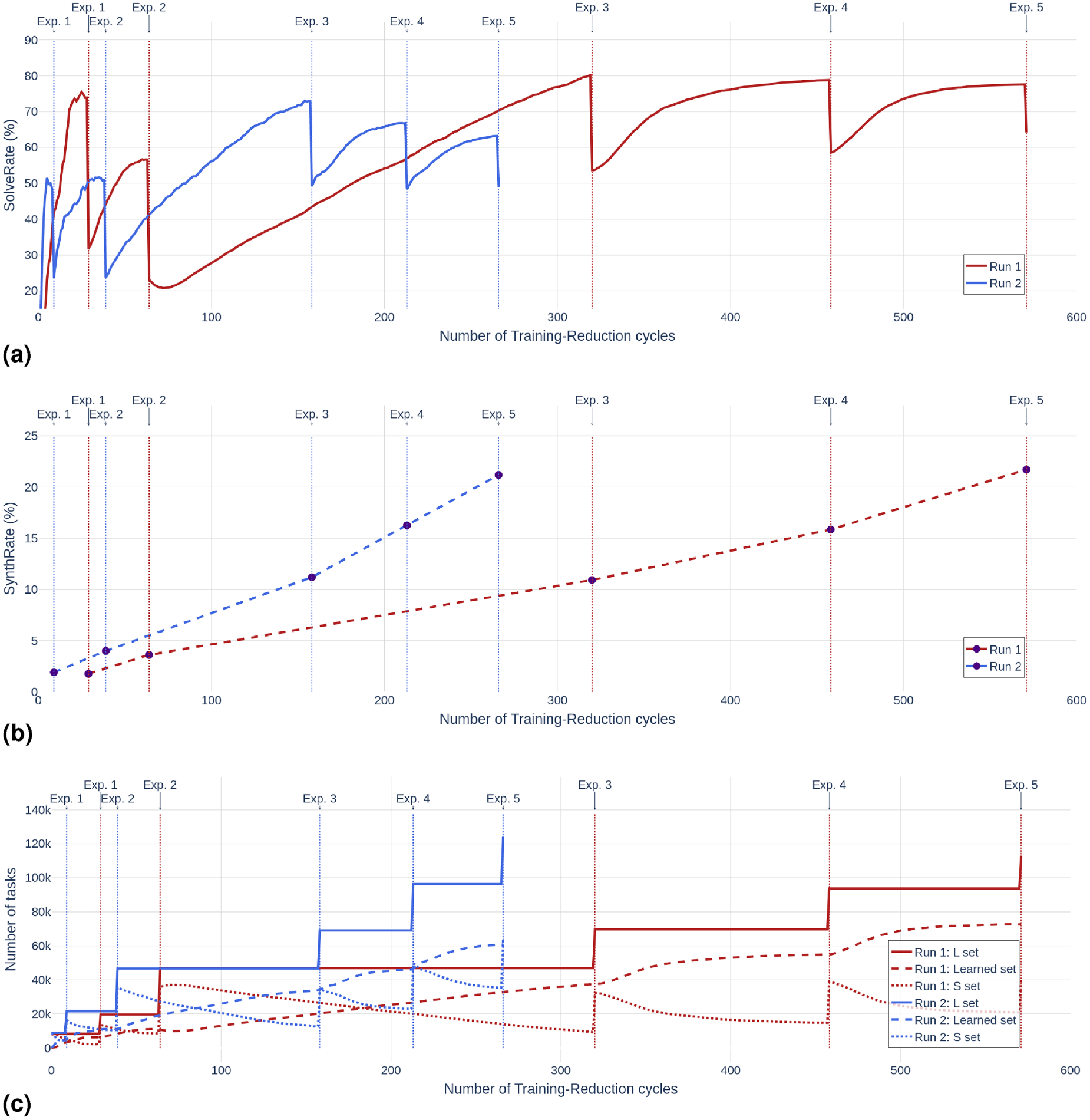
The dynamics of two runs of TransCoder that used different random initializations. Vertical lines indicate the activations of the Exploration phase. Run 1 and Run 2 lasted 4 and 2 days, respectively, on NVIDIA A100 GPUs. (a) SolveRate—the success rate on a set of tasks that dynamically changes during training; (b) SynthRate—the success rate on a precomputed, fixed set of 205,745 synthetic tasks. (c) The number of tasks in the working training set L, in the set of solved tasks S, and the number of learned tasks. Once a task has been solved, it is moved from S to the learned set, hence the total size of these both sets remains constant within a given outer cycle of the method.

The continuous lines in Figure 7(a) show SolveRate, the percentage of tasks solved, estimated from a random sample drawn from the current set $S$ . Because $S$ varies dynamically along training, this quantity is not objective, yet it illustrates the dynamics of training. The sudden drops in performance occur right after the completion of the Exploration phase, which augments $S$ with new tasks that the method cannot yet solve. Notice, however, that, at least for Run 1, the drops tend to be less prominent in consecutive cycles, which may signal that TransCoder gradually improves its skills of solving the newly generated synthetic tasks.

To provide a more objective assessment, the dashed lines in Figure 7(b) present SynthRate, the percentage of tasks solved from a precomputed suite of over 200k synthetic tasks. The curves of this metric exhibit fast and steady growth, demonstrating TransCoder’s capacity for continuous progress. Importantly, for both runs, these curves do not tend to saturate, suggesting the potential for additional increase upon further continuation of training.

Figure 7(c) presents the dynamics of the working sets of tasks manipulated in TransCoder, synced in time with Figures 7(a) and 7(b). Each invocation of the Exploration phase expands the working set of tasks $S$ (dotted line) and the $L$ set (solid line). In the Training-Reduction iterations that follow, TransCoder gradually learns to solve those tasks, which causes those solved ones to be removed from $S$ and added to the “learned” set (dashed lines).

The primary feature distinguishing Run 1 from Run 2 is that the latter tended to “consume” (i.e., successively learn to solve) the tasks from $S$ at a higher average rate than the former. This is particularly evident in the third cycle of both runs (after Exp. 2), which lasts over 350 Training-Reduction cycles for Run 1, while only slightly more than 100 cycles for Run 2. This tendency causes Run 2 to invoke the Exploration phase more often, and, as a result, expose TransCoder to new tasks earlier in the process. This, in turn, leads also to faster growth of the $L$ set for Run 2.

Another difference between Run 1 and Run 2 is that the former one tends to “exhaust” its working set $S$ almost entirely toward the end of each cycle, while for Run 2, each cycle ends with $S$ still holding a substantial number of tasks. It is tempting to hypothesize that this helped Run 2 to make faster progress and ultimately achieve almost the same value of SynthRate as Run 1 (almost 21.2% vs. $\sim$ 21.7%), yet at a much lower computational expense ( $\sim$ 260 cycles vs. almost 700 cycles). This claim needs, however, to be verified in a separate study.

Table 5 presents the metrics at the completion of consecutive training cycles of Run 1 (cf. Figure 6). The monotonous increase of SynthRate also positively impacts the ARCRate, which ultimately achieves the all-high value of 3% at the end of the run, suggesting that the skills learned from the synthetic, easier tasks translate into more effective solving of the harder original ARC tasks.

Table 5.

SynthRate and ARCRate Immediately Before the Commencement of Particular Training Cycles (i.e., Before Exploration Phases), for Run 1.

Cycle	1	2	3	4	5
SynthRate	1.77%	3.61%	10.93%	15.86%	21.72%
ARCRate	1.75%	2.00%	2.25%	2.75%	3.00%

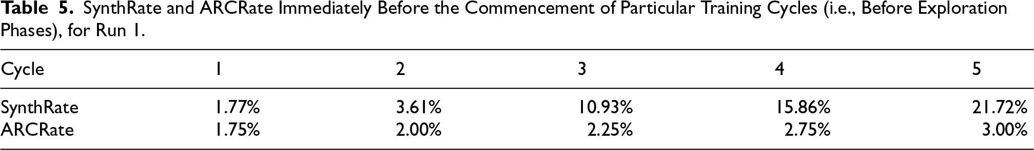
Table 6 presents the results in terms of historical progress, that is, how TransCoder fares in consecutive cycles on the synthetic tasks it generated in the previous cycles. This concept has been introduced in Miconi (2009) to assess the progress on coevolutionary algorithms in the absence of well-defined objective yardsticks. The table shows the rate of solved programs achieved by the snapshots of TransCoder trained for a given number of cycles (in rows) on the tasks from $S$ collected in particular cycles (in columns).⁸ Similarly to previous results, the table demonstrates overall consistent improvement of the model’s performance. The success rate on $S$ collected in the first cycle (first column) is noticeably high, which we attribute to the fact that in this initial cycle, the method produces the simplest, and thus the easiest, synthetic tasks. Compared to them, the rates in the second column tend to be lower, but then experience a monotonous increase until the diagonal of the table. This indicates that the knowledge acquired by TransCoder in previous cycles is not forgotten and helps it solve the “historical” tasks even if they are not part of its working training set anymore. The success rates right off the diagonal are much lower, which was expected, as they mark the performance on the synthetic tasks that TransCoder has not yet trained on.

Table 6.

Performance of the Snapshots of the Model From a Given Cycle (row) on the Synthetic Examples Collected in a Given Cycle (column), for Run 1.

	Synthetic Task Set $S$ From Cycle
TransCoder’s Snapshot From Cycle	1	2	3	4	5
1	41.12%	1.18%	0.16%	0.03%	0.02%
2	34.09%	40.42%	0.06%	0.04%	0.00%
3	40.62%	32.92%	55.33%	0.78%	0.38%
4	42.02%	23.57%	47.69%	56.31%	0.86%
5	36.66%	24.10%	44.00%	52.84%	58.47%

Note. For Instance, TransCoder From the First Cycle (the First row in the Table) Solves 41.12% of the Synthetic Tasks Created in the Same Cycle, 1.18% of the Tasks Created in the Second Cycle, 0.16% From the Third Cycle, 0.03% From the Fourth Cycle, and 0.02% From the Fifth Cycle.

Table 7.

The List of Predefined Symbol Keys Available in the Domain-Specific Language (DSL).

Name	Type	Description
Zero	Int	A constant “0”
One	Int	A constant “1”
Horizontal	Orientation	A categorical value used for the Flip operation
Vertical	Orientation	A categorical value used for the Flip operation
N4	Connectivity	A categorical value used for the FloodFill operation
N8	Connectivity	A categorical value used for the FloodFill operation
Cw	Direction	A categorical value used for the Rotate operation
Ccw	Direction	A categorical value used for the Rotate operation
Black	Color	A categorical value of color from ARC
Blue	Color	A categorical value of color from ARC
Red	Color	A categorical value of color from ARC
Green	Color	A categorical value of color from ARC
Yellow	Color	A categorical value of color from ARC
Grey	Color	A categorical value of color from ARC
Fuchsia	Color	A categorical value of color from ARC
Orange	Color	A categorical value of color from ARC
Teal	Color	A categorical value of color from ARC
Brown	Color	A categorical value of color from ARC
Scene	Region	A Region representing input raster from an input-output demonstration pair
Functional Input	–	A special key available only during execution/generation of functional operation subprogram

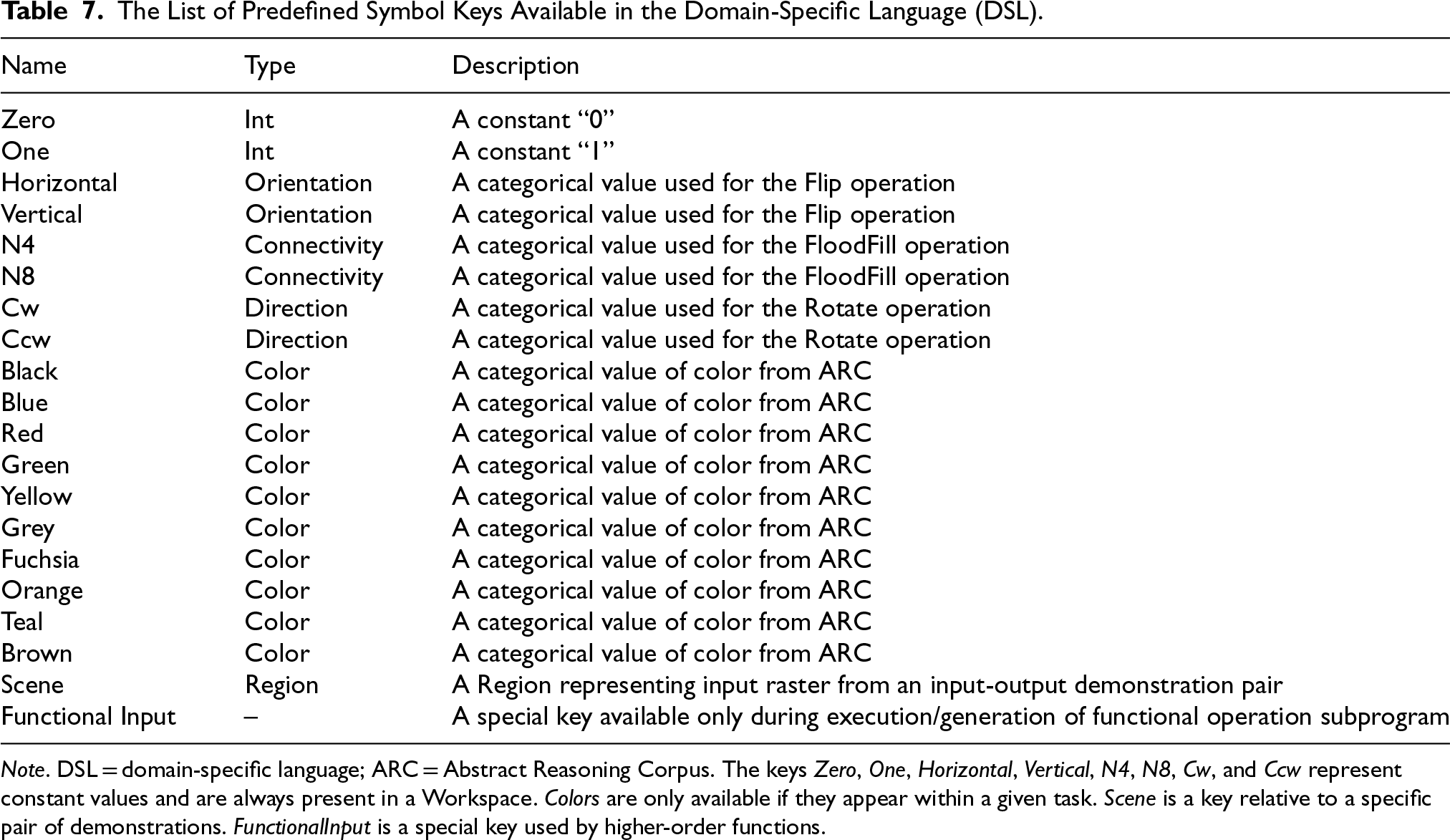
Note. DSL = domain-specific language; ARC = Abstract Reasoning Corpus. The keys Zero, One, Horizontal, Vertical, N4, N8, Cw, and Ccw represent constant values and are always present in a Workspace. Colors are only available if they appear within a given task. Scene is a key relative to a specific pair of demonstrations. FunctionalInput is a special key used by higher-order functions.

Table 8.

Definitions of the Operations Available in the Domain-Specific Language (DSL).

Name	Signature	Description
Add	(A: Arithmetic, A: Arithmetic) ->A: Arithmetic	Adds two objects of the same type inheriting from Arithmetic
Area	(Region) ->Int	Calculates the surface area of a region
Crop	(Region, Loc, Loc) ->Region	Cuts a subregion based on the top left and bottom right vertices
Deduplicate	(List[A]) ->List[A]	Removes duplicates from the list
Diff	(List[A], List[A]) ->List[A]	Performs a difference operation on two lists
Draw	(Region, Union[Region, List[Region]]) ->Region	Overlays a Region or list of Regions on the given input region
Equals	(A, A) ->Bool	Compares two objects of the same type
Filter	(List[A], (A->Bool)) ->List[A]	Filters the list of input objects based on the result of the subroutine run on each input element
First	(Pair[A, Type]) ->A	Gets the first element of the input pair
Flip	(Region, Orientation) ->Region	Performs a vertical or horizontal flip of the input region
FloodFill	(Region, Color, Connectivity) ->List[Region]	Performs segmentation of the input Region using the Flood Fill algorithm and the background color and neighborhood type (n4 or n8)
GroupBy	(List[A], (A->B)) ->List[Pair[B, List[A]]]	Groups objects from the input list based on the results of the subroutine
Head	(List[A]) ->A	Gets the first element of the input list
Height	(Region) ->Int	Returns the height of the region
Intersection	(List[A], List[A]) ->List[A]	Returns the intersection of two lists
LBC	(Region) ->Loc	Returns the location of the left bottom corner
LTC	(Region) ->Loc	Returns the location of the left top corner
Len	(List[Type]) ->Int	Returns the length of the input list
Line	(Loc, Loc, Color) ->Region	Creates a single-color Region that represents a line between two points
Loc	(Int, Int) ->Loc	Location object constructor
Map	(List[A], (A->B)) ->List[B]	Performs the transformation operation of each element of the input list using a subroutine
MostCommon	(List[A], (A->B)) ->B	Returns the most frequently occurring object from the input list based on the value returned by the subroutine applied to the list elements
Neg	(Union[A, B: Bool]) ->Union[A, B: Bool]	Performs a negation operation on the input object
Paint	(Region, Color) ->Region	Colors the input region a solid color
Pair	(A, B) ->Pair[A, B]	The constructor of an object of type Pair
Pixels	(Region) ->List[Region]	Returns a list of pixels of the input region
RBC	(Region) ->Loc	Returns the location of the right bottom corner
RTC	(Region) ->Loc	Returns the location of the right top corner
Rect	(Loc, Loc, Color) ->Region	Creates a single-color Region representing a rectangle bounded by the input locations
Reverse	(List[A]) ->List[A]	Reverses the input list
Rotate	(Region, Direction) ->Region	Rotates the Input Region clockwise or counterclockwise
Scale	(Region, Union[Int, Pair[Int, Int]]) ->Region	Scales the input Region according to the integer argument
Second	(Pair[Type, A]) ->A	Returns the second element of the input pair
Shift	(Region, Union[Loc, Pair[Int, Int]]) ->Region	Shifts the input Region by an integer argument
Sort	(List[A], (A->Comparable) ->List[A]	Sorts the input list based on the result of the subroutine applied to the list
Sub	(A: Arithmetic, A: Arithmetic) ->A: Arithmetic	Subtracts two objects of the same type inheriting from Arithmetic
Tail	(List[A]) ->A	Gets the last element of the input list
Union	(List[A], List[A]) ->List[A]	Returns the sum of two input lists
Width	(Region) ->Int	Returns the width of the region
Zip	(List[A], List[B]) ->List[Pair[A, B]]	Creates a list of pairs of corresponding elements in the input lists

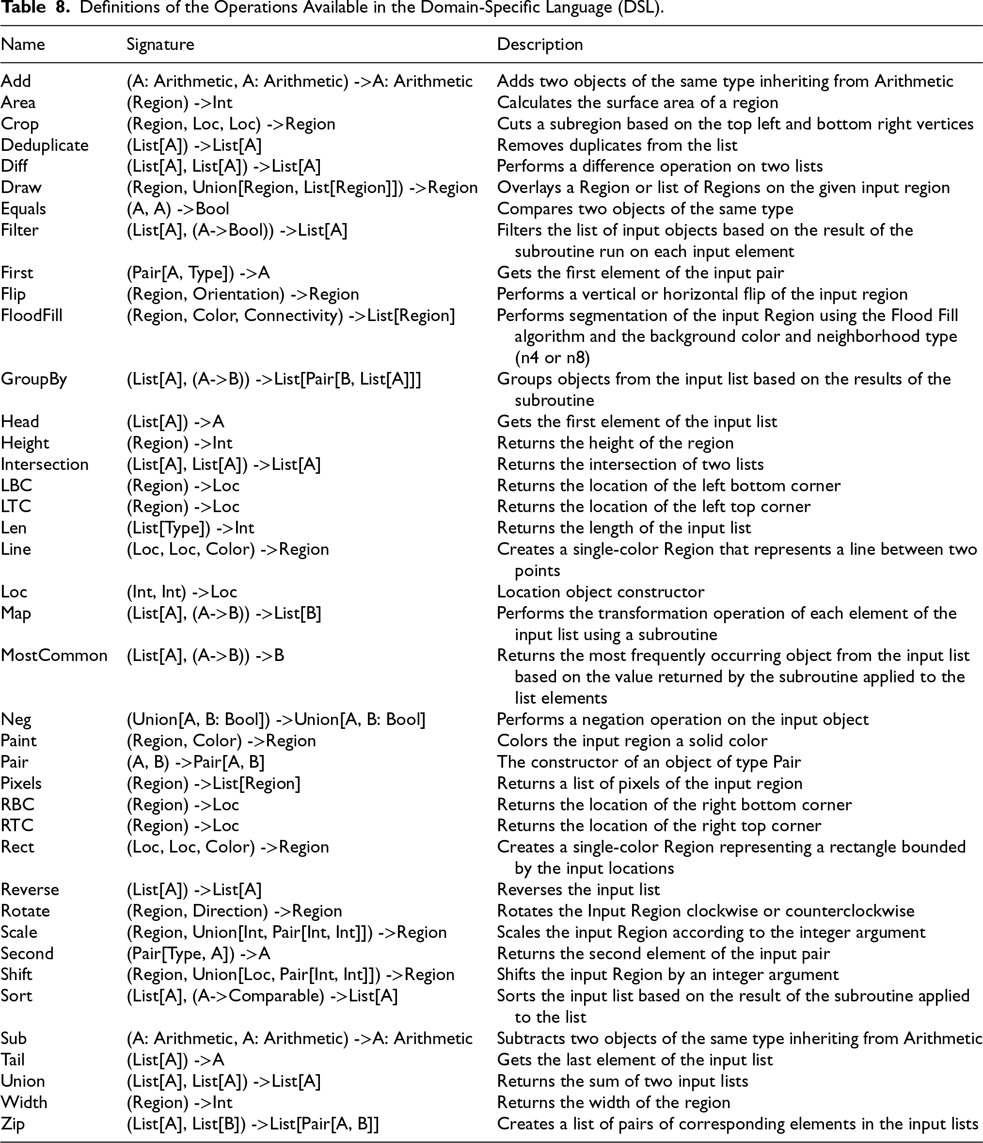
Figure 8 shows examples of generated tasks with solutions, that is, the $(T, p)$ pairs added to $S$ during training. The left-hand program first fills the scene (which initially has the same dimensions as the input raster) with the red color. Then, it “measures” the height of the input raster by locating its left bottom corner (the LBC function), which will in general have coordinates $(0, y_{max)}$ (the coordinates are 0-based). Finally, it crops the scene to the rectangle that spans from this point/corner to $(1, 1)$ . The resulting output raster will thus be a rectangle that is always two pixels wide, while its height is smaller by one than the input raster. The program synthesized for the right-hand task shown in Figure 8 also involves cropping of the input raster, but the extent of the cropping rectangle is determined in a more complex fashion, by flood-filling the input raster and locating the first pixel of the resulting region. Examples of programs that create new synthetic problems from subsequent Exploration phases are presented in Table 9.

Figure 8.

Examples of (task, program) pairs synthesized by the model.

Table 9.

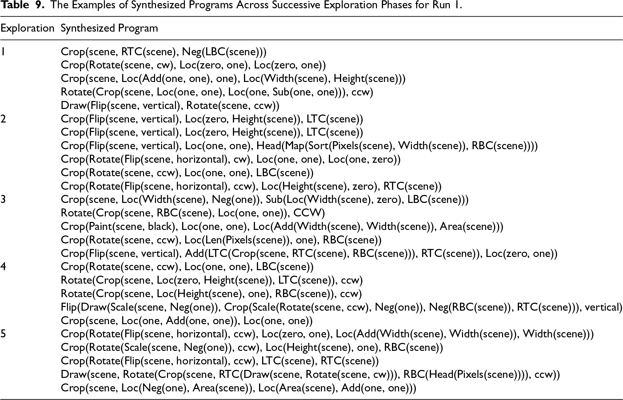
The Examples of Synthesized Programs Across Successive Exploration Phases for Run 1.

Exploration	Synthesized Program
1	Crop(scene, RTC(scene), Neg(LBC(scene)))
	Crop(Rotate(scene, cw), Loc(zero, one), Loc(zero, one))
	Crop(scene, Loc(Add(one, one), one), Loc(Width(scene), Height(scene)))
	Rotate(Crop(scene, Loc(one, one), Loc(one, Sub(one, one))), ccw)
	Draw(Flip(scene, vertical), Rotate(scene, ccw))
2	Crop(Flip(scene, vertical), Loc(zero, Height(scene)), LTC(scene))
	Crop(Flip(scene, vertical), Loc(zero, Height(scene)), LTC(scene))
	Crop(Flip(scene, vertical), Loc(one, one), Head(Map(Sort(Pixels(scene), Width(scene)), RBC(scene))))
	Crop(Rotate(Flip(scene, horizontal), cw), Loc(one, one), Loc(one, zero))
	Crop(Rotate(scene, ccw), Loc(one, one), LBC(scene))
	Crop(Rotate(Flip(scene, horizontal), ccw), Loc(Height(scene), zero), RTC(scene))
3	Crop(scene, Loc(Width(scene), Neg(one)), Sub(Loc(Width(scene), zero), LBC(scene)))
	Rotate(Crop(scene, RBC(scene), Loc(one, one)), CCW)
	Crop(Paint(scene, black), Loc(one, one), Loc(Add(Width(scene), Width(scene)), Area(scene)))
	Crop(Rotate(scene, ccw), Loc(Len(Pixels(scene)), one), RBC(scene))
	Crop(Flip(scene, vertical), Add(LTC(Crop(scene, RTC(scene), RBC(scene))), RTC(scene)), Loc(zero, one))
4	Crop(Rotate(scene, ccw), Loc(one, one), LBC(scene))
	Rotate(Crop(scene, Loc(zero, Height(scene)), LTC(scene)), ccw)
	Rotate(Crop(scene, Loc(Height(scene), one), RBC(scene)), ccw)
	Flip(Draw(Scale(scene, Neg(one)), Crop(Scale(Rotate(scene, ccw), Neg(one)), Neg(RBC(scene)), RTC(scene))), vertical)
	Crop(scene, Loc(one, Add(one, one)), Loc(one, one))
5	Crop(Rotate(Flip(scene, horizontal), ccw), Loc(zero, one), Loc(Add(Width(scene), Width(scene)), Width(scene)))
	Crop(Rotate(Scale(scene, Neg(one)), ccw), Loc(Height(scene), one), RBC(scene))
	Crop(Rotate(Flip(scene, horizontal), ccw), LTC(scene), RTC(scene))
	Draw(scene, Rotate(Crop(scene, RTC(Draw(scene, Rotate(scene, cw))), RBC(Head(Pixels(scene)))), ccw))
	Crop(scene, Loc(Neg(one), Area(scene)), Loc(Area(scene), Add(one, one)))

6. Conclusions and Future Work

This study corroborated our preliminary findings from Bednarek and Krawiec (2024) and confirmed TransCoder’s capacity to provide itself with a learning gradient by generating synthetic tasks of moderate difficulty, which close the “skill gap” existing between the capabilities of an initial untrained and inexperienced solver and the difficulty of ARC tasks. Crucially, the generative aspect of this architecture, combined with expressing candidate solutions in a DSL, allows the method to obtain concrete DSL programs, use them as concrete targets for the synthesis process (Generator), and so gradually transform an unsupervised learning problem into a supervised one. As evidenced by the experiment, SL facilitated in this way provides informative learning guidance, unparalleled when compared to RL we engaged in preliminary experiments.

In a sense, this research is venturing into the domain of relational learning and, by employing deep learning components to this aim, explores the area of relational deep learning (see, e.g., Fey et al., 2024). In the current architecture of TransCoder, this is achieved with the quite rudimentary means of a variational layer, which allows us to relate, in a many-to-many, bi-directional fashion, the ARC tasks to the DSL programs that solve them. Prospectively, it would be interesting to engage other mechanisms for this purpose, perhaps such that allow discarding the, not necessarily desirable, stochasticity of the variational mapping.

The modularity of the proposed architecture allows TransCoder to be adapted to other types of data than those considered in our DSL and, more generally, than those specific to the realm of ARC tasks. In particular, the Solver and Generator modules are independent of the input data type, while the only type-specific module is Perception. This ensures relatively loose coupling between the method and the DSL, and facilitates introducing changes in the latter, or even replacing it entirely. Future work will include applying the approach to other benchmarks in different domains, developing alternative DSLs, transferring abstraction and reasoning knowledge between datasets, and prioritizing the search in the solution space to solve the original ARC tasks.

Footnotes

Funding

The authors disclosed receipt of the following financial support for the research, authorship, and/or publication of this article: The performance of the snapshots of the model was derived from TAILOR, a project funded by EU Horizon 2020 research and innovation program under GA No. 952215, by the statutory funds of Poznan University of Technology and the Polish Ministry of Education and Science grant no. 0311/SBAD/0770.

Declaration of Conflicting Interests

The authors declared no potential conflicts of interest with respect to the research, authorship, and/or publication of this article.

ORCID iDs

Jakub Bednarek

Krzysztof Krawiec

Notes

Appendix

References

Abadi

Barham

Chen

Davis

Dean

Devin

Ghemawat

Irving

Isard

Kudlur

Levenberg

Monga

Moore

Murray

D. G.

Steiner

Tucker

P. A.

Vasudevan

Warden

Zhang

(2016). Tensorflow: A system for large-scale machine learning. CoRR abs/1605.08695. http://arxiv.org/abs/1605.08695

Alford

Gandhi

Rangamani

Banburski

Wang

Dandekar

Chin

Poggio

T. A.

Chin

(2021). Neural-guided, bidirectional program search for abstraction and reasoning. CoRR abs/2110.11536. https://arxiv.org/abs/2110.11536

Alvarez-Melis

Jaakkola

T. S.

(2017). Tree-structured decoding with doubly-recurrent neural networks. In International conference on learning representations. https://openreview.net/forum?id=HkYhZDqxg

Assouel

Rodriguez

Taslakian

Vazquez

Bengio

(2022). Object-centric compositional imagination for visual abstract reasoning. In ICLR2022 workshop on the elements of reasoning: Objects, structure and causality. https://openreview.net/forum?id=rCzfIruU5x5

Bednarek

Krawiec

(2024). Learning to solve abstract reasoning problems with neurosymbolic program synthesis and task generation. In T. R. Besold, A. d’Avila Garcez, E. Jimenez-Ruiz, R. Confalonieri, P. Madhyastha, & B. Wagner (Eds.), Neural-symbolic learning and reasoning (pp. 386–402). Springer Nature Switzerland.

Bednarek

Piaskowski

Krawiec

(2018). Ain’t nobody got time for coding: Structure-aware program synthesis from natural language. CoRR abs/1810.09717. http://arxiv.org/abs/1810.09717

Bongard

M. M.

(1967). The problem of recognition. M.: Nauka.

Chaudhuri

Ellis

Polozov

Singh

Solar-Lezama

Yue

(2021). Neurosymbolic programming. Foundations and Trends in Programming Languages, 7(3), 158–243. https://doi.org/10.14461561/2500000049. https://www.nowpublishers.com/article/Details/PGL-049

Chollet

(2019). On the measure of intelligence. CoRR abs/1911.01547. http://arxiv.org/abs/1911.01547

10.

Dosovitskiy

Beyer

Kolesnikov

Weissenborn

Zhai

Unterthiner

Dehghani

Minderer

Heigold

Gelly

Uszkoreit

Houlsby

(2020). An image is worth

16 \times 16

words: Transformers for image recognition at scale. CoRR abs/2010.11929. https://arxiv.org/abs/2010.11929

11.

Ellis

Wong

Nye

Sablé-Meyer

Morales

Hewitt

Cary

Solar-Lezama

Tenenbaum

J. B.

(2021). Dreamcoder: Bootstrapping inductive program synthesis with wake-sleep library learning. In Proceedings of the 42nd ACM SIGPLAN international conference on programming language design and implementation, PLDI 2021 (pp. 835–850). Association for Computing Machinery. https://doi.org/10.1145/3453483.3454080

12.

Ferré

(2021). First steps of an approach to the ARC challenge based on descriptive grid models and the minimum description length principle. CoRR abs/2112.00848. https://arxiv.org/abs/2112.00848

13.

Fey

Huang

Lenssen

J. E.

Ranjan

Robinson

Ying

You

Leskovec

(2024). Position: Relational deep learning - graph representation learning on relational databases. In R. Salakhutdinov, Z. Kolter, K. Heller, A. Weller, N. Oliver, J. Scarlett, & F. Berkenkamp (Eds.), Proceedings of the 41st international conference on machine learning (PMLR, Vol. 235, pp. 13592–13607). PMLR. https://proceedings.mlr.press/v235/fey24a.html

14.

Hofstadter

D. R.

(1995). Fluid concepts & creative analogies: Computer models of the fundamental mechanisms of thought. Basic Books.

15.

Johnson

Hariharan

van der Maaten

Fei-Fei

Zitnick

C. L.

Girshick

R. B.

(2016). CLEVR: A diagnostic dataset for compositional language and elementary visual reasoning. CoRR abs/1612.06890. http://arxiv.org/abs/1612.06890

16.

Kingma

D. P.

Welling

(2022). Auto-encoding variational bayes.

17.

Lin

Chen

Yan

(2014). Network in network. https://arxiv.org/abs/1312.4400

18.

Loshchilov

Hutter

(2017). Fixing weight decay regularization in Adam. CoRR abs/1711.05101. http://arxiv.org/abs/1711.05101

19.

Mao

Gan

Kohli

Tenenbaum

J. B.

(2019). The neuro-symbolic concept learner: Interpreting scenes, words, and sentences from natural supervision. arXiv:1904.12584 [cs] http://arxiv.org/abs/1904.12584

20.

Miconi

(2009). Why coevolution doesn’t “work“: superiority and progress in coevolution. In L. Vanneschi, S. Gustafson, A. Moraglio, I. De Falco, & M. Ebner (Eds.), Proceedings of the 12th European conference on genetic programming, EuroGP 2009 (LNCS, vol. 5481, pp. 49–60). Springer. https://doi.org/10.1007/978-3-642-01181-8_5. http://www.cs.bham.ac.uk/ txm/eurogp09.pdf

21.

Mirchandani

Xia

Florence

Ichter

Driess

Arenas

M. G.

Rao

Sadigh

Zeng

(2023). Large language models as general pattern machines. https://arxiv.org/abs/2307.04721

22.

Moskvichev

Odouard

V. V.

Mitchell

(2023). The conceptarc benchmark: Evaluating understanding and generalization in the arc domain. https://arxiv.org/abs/2305.07141

23.

Muggleton

S. H.

Watanabe

(2014). Latest advances in inductive logic programming. Imperial College Press. https://doi.org/10.1142/p954. https://www.worldscientific.com/doi/abs/10.1142/p954

24.

Smith

L. N.

(2018). A disciplined approach to neural network hyper-parameters: Part 1 – learning rate, batch size, momentum, and weight decay. CoRR abs/1803.09820. http://arxiv.org/abs/1803.09820

25.

Vaswani

Shazeer

Parmar

Uszkoreit

Jones

Gomez

A. N.

Kaiser

Polosukhin

(2017). Attention is all you need. CoRR abs/1706.03762. http://arxiv.org/abs/1706.03762

26.

Khalil

E. B.

Sanner

(2022). Graphs, constraints, and search for the abstraction and reasoning corpus. https://arxiv.org/abs/2210.09880

27.