Neural networks for wind power generation forecasting in Uruguay

Abstract

This article explores the application of Artificial Neural Networks in predicting wind power generation. The precise prediction of power output is crucial for establishing a reliable wind power generation framework. Accurate forecasts play a key role in enabling efficient planning, management, and distribution strategies for the generated power, leading to improved performance of electrical systems. A specific case study is addressed: the nation-wide wind power generation in Uruguay. The study considers real wind power generation data from Uruguay, spanning the period from 2018 to 2022. The forecasting is carried out using different artificial neural network architectures, including Convolutional Neural Network, Long Short-Term Memory artificial neural network, Encoder-Decoder architectures, and hybrid models. Univariate and multivariate models are studied. The main results indicate that the best proposed hybrid approach demonstrates high prediction accuracy, with a median root mean square error of 0.12, median absolute error of 0.09, and mean absolute percentage error of 14.9%, significantly improving over other models. The computed forecasts can be effectively utilized for planning and scheduling to enhance the quality of services provided by the smart electric grid.

Introduction

Renewable energy sources, including wind and solar power, have become increasingly crucial for their role in diminishing greenhouse gas emissions, which is critical in the battle against climate change. Nevertheless, the incorporation of renewable energy sources into the power grid encounters obstacles stemming from their variability, intermittent nature, and limited predictability (Halamay and Brekken, 2010). In this regard, wind power is considered one of the more challenging renewable energy sources to predict accurately. due to its inherent variability and intermittency (Sulaiman and Mustaffa, 2024). Unlike traditional (non-renewable) power sources like coal or natural gas, which can be controlled to meet demand, the availability and strength of wind are influenced by weather patterns and can fluctuate unpredictably. The variability of wind is caused by a range of factors, including changes in atmospheric pressure, temperature gradients, and local topography. These variables make it difficult to forecast how much electricity a wind turbine will generate in a given period of time. Efforts to improve the predictability of wind power generation have been ongoing, with advancements in weather forecasting technologies and the development of sophisticated prediction models. By using data from weather stations, satellites, and on-site sensors, researchers and engineers are working to enhance the accuracy of wind power generation forecasts (Tsai et al., 2023).

Despite its inherent challenges, wind power continues to play a significant role in the transition to cleaner energy sources. As technology and forecasting methods improve, the predictability of wind power generation is expected to increase, making it a more reliable and efficient component of the energy grid. Forecasts are indispensable for facilitating the seamless integration into smart grid functionalities, enhancing energy control, and guaranteeing the stability and dependability of the electrical grid (Worighi et al., 2019).

Over the past two decades, significant progress has been made in forecasting models for renewable energy generation (Hasanuzzaman and Abd Rahim, 2020). The proposed forecasting models leverage a variety of data sources, including historical information of energy production, weather predictions, topographic data, and other pertinent information. Soft computing and computational intelligence are instrumental in ensuring precision of forecasting renewable energy sources output (Benti et al., 2023; Zhang et al., 2022b). These methods take advantage of their ability to handle uncertainty, tolerate faults, handle non-linearity and emulate human reasoning, for providing robustness and efficacy to solve complex forecasting problems (Liu et al., 2025).

The advantages of accurate forecasts for renewable energy generation are considerable, encompassing improvements in grid reliability, reduced energy expenses, and enhanced integration of renewable energy sources. In particular, precise forecasting of power generation is pivotal in the development of dependable photovoltaic systems. This capability facilitates efficient planning, control, and distribution of generated power, thereby guaranteeing optimal system performance and effectiveness (Dashti and Rouhandeh, 2023; Dudek et al., 2023; Wang et al., 2022).

In this line of work, this article delves into the application of computational intelligence/machine learning models, with a specific focus on Artificial Neural Networks (ANN), for the prediction of wind power generation. The research examines a particular real-world case study involving the prediction of wind power generation at national level, in Uruguay. Real data is used to that end, including historical information about wind power generation, estimations based on weather data, and other relevant information. The study was performed in a collaborative effort between Universidad de la República, Uruguay, and the Uruguayan electricity company (Administración Nacional de Usinas y Trasmisiones Eléctricas, UTE), aimed at exploring the implementation of computational intelligence/machine learning models and their incorporation into operational and decision-making tools for smart grid systems. The research integrates diverse data sources, leveraging actual data collected over the period spanning from 2018 to 2022.

The analysis explores various ANN architectures: multi-layer perceptron (MLP), Convolutional Neural Networks (CNN), Long Short Term Memory (LSTM), and hybrid models convolutional LSTM (C-LSTM) and Encoder-Decoder LSTM (ED-LSTM). The studied architectures undergo evaluation based on their efficacy in addressing the given problem. The experimental evaluation of the studied computational intelligence techniques illustrates their effectiveness in predictive modelling. The key results indicate that the hybrid ED-LSTM model achieved an average Root Mean Square Error (RMSE) metric of 0.12, Mean Absolute Error (MAE) of 0.09, and Mean Absolute Percentage Error (MAPE) of 14.9%, showcasing competitiveness with outcomes from relevant literature and outperforming other ANN models considered in the study. The forecasts generated serve as valuable inputs for decision making, operational and stochastic optimization models, enriching the planning and scheduling processes and ultimately enhancing the quality of service provided by the electricity grid to the population.

This article extends our previous conference manuscript “Wind power generation forecasting: a real-world nation-wide case study in Uruguay” (Nesmachnow and Risso, 2025), presented at VII Iberoamerican Congress on Smart Cities (ICSC-CITIES). The conference manuscript studied two initial variants of LSTM for wind power generation forecasting. Novel scientific contributions in this article consist of: i) a detailed explanation of the problem at hand and the data considered in the case study, ii) an expanded review of pertinent literature, including recent articles on the topic, iii) the analysis of five ANN architectures, including hybrid methodologies, in univariate and multivariate versions, iv) a comprehensive experimental assessment of the studied models, ncluding hyperparameters tunning, and v) the comparative evaluation of the best ANN model for forecasting wind power generation for the real case study in Uruguay. The new model from this article significantly enhances the forecasting accuracy when compared to the LSTM methods presented in the previous conference article.

The article is organized as follows. An outline of the renewable energy generation forecasting problem is presented on the next section, incorporating a review of pertinent literature and particular works that focused on the Uruguay case study. The following section details the applied methodology and provide comprehensive insights into the implemented ANN-based forecasting models. Subsequently, the article presents the experimental assessment of the proposed approach for forecasting wind power generation. The results obtained are documented and deliberated upon. Finally, the concluding section describes the research findings and delineates potential lines for future research.

Forecasting wind power generation

This section presents the main features of the forecasting problem under consideration and examines pertinent research studies in the subject of forecasting wind power generation.

Problem description

Predicting power generation is a pivotal issue within the emerging smart grid paradigm (Alsirhani et al., 2023; Kaur et al., 2022). Precise forecasting aids in mitigating the effects of variability on critical aspects linked to prevalent strategies in smart grids, such as demand-side management, optimized power flow, load shedding, and predictive analytics. An essential problem in nowadays data-centric smart grid setups involves properly handling forecasting methods, curbing prediction inaccuracies, all while considering the intrinsic uncertainty associated with renewable energy sources. This quest is fundamental for dealing with challenges and guaranteeing the efficient functioning of the smart grid.

The main focus of this research centres on predicting the time series data pertaining to wind power generation in Uruguay. This forecast is performed using computational intelligence methods and authentic data supplied by the national electricity provider, UTE. UTE has led the way in endeavours related to forecasting renewable energy in Uruguay. Employing a blend of weather prediction models, historical energy production data, and machine learning algorithms, UTE achieves a high level of precision in projecting renewable energy generation. The advantages stemming from the forecasting initiatives are manifold, encompassing enhanced grid dependability, diminished energy expenditures, and heightened integration of renewable energy sources. These results are crucial considering the notable progress made by Uruguay in its shift towards renewable energy sources within its electricity grid. With electricity generation from renewable sources surpassing 85% of the energy portfolio, and a record of 94% between 2018 and 2022 (Uruguay XXI, 2023), Uruguay stands as one of the leader countries worldwide in terms of renewable energy utilization. Leveraging efficient forecasting mechanisms for renewable energy production facilitates the enhancement and fine-tuning of operational models, guaranteeing dependable and top-tier service aligned with smart grid principles (Aguiar and Pérez, 2023). The precise forecasting of renewable energy generation stands as a crucial component for the progression of Uruguay towards a more sustainable and dependable energy framework. The advances of the nation in this domain serve as a blueprint for other countries aspiring to incorporate renewable energy sources into their power grids.

Problem features

In the addressed real-world Uruguayan case study, the goal is to generate accurate forecasts for every hour over a three-day span (72 hours), as forecasts are required to ensure precise and effective scheduling and distribution of available electricity generation resources to meet the demand in the country. Forecasts are critical for making well-informed decisions within the power system and optimizing the use of resources efficiently. The associated scheduling and control challenges concerns the management and the operation of power plants, which entails determining the suitable power output for each plant and dispatching the electricity produced to fulfill the load requirements. This task is fundamental in guaranteeing the dependable and effective operation of the power grid. By reducing costs, improving grid reliability, and aiding the integration of renewable energy sources, the scheduling and control issue plays a key role in enhancing the overall efficiency of the power system.

Since the considered forecasting horizon includes multiple hourly predictions, it is a case of medium-to-long term forecasting problem (Ahmed et al., 2020; Ren et al., 2015). Even though larger renewable energy generation forecasting problems have been solved, with forecasting horizons over one week and even months, they are not common for wind power generation. The main reason is that the wind resource has a very high variability, which makes it very difficult to estimate in the long term. In turn, for wind power is very hard to take advantage of information about seasonal variations and specific climate or generation patterns, unlike in the case of solar power generation, which tends to have a significantly more regular and smooth pattern during the year.

Forecasting over multiple hours poses a significantly more intricate challenge when contrasted with single-hour or shorter-to-medium term wind power generation forecasting, typically conducted within a forecast horizon of one or a few hours, as examined in related researches. The forecasting technique must predict a sequence of consecutive values within the wind power generation time series.

Problem data

The main source of data used for training and validation of the proposed ANN-based wind power generation forecasting models is the historical database of wind power generation from the more than 40 wind farms deployed in the country. Data were gathered by the Supervisory Control And Data Acquisition (SCADA) system of UTE. A complete description of the wind power generation dataset is presented in the experimental evaluation section.

For the multivariate models, estimations computed based on state-of-the-art numerical weather prediction models are also considered. Intuitively, these additional data help guiding the ANN-based forecasting models studied in the article.

Literature review: state-of-the-art

Numerous scholarly articles have explored various aspects and variants of the wind power generation forecasting problem, recognizing its significance for the management and functioning of electricity systems.

Early articles reviewing the application of forecasting models for wind power generation confirmed that the prediction error significantly increases when considering larger time forecasting horizons. For instance, the Wind Power Management System commercial model was able to achieve excellent accuracy (i.e., RMSE between 7%–19%) for immediate and short-term prediction. The Armines Wind Power Prediction System software achieved accuracy values from 5% of the nominal power for a single farm for one-hour ahead predictions to 15% for 48 hours ahead predictions (Monteiro et al., 2009). Similar values were obtained using other numerical forecasting tools, e.g., eWind/TureWind 11.7% for one-day ahead forecasting using physical and statistical models (Wang et al., 2021), WPFSis with an accuracy of 16 to 19% (Chen et al., 2017).

Computational intelligence and machine learning methods have also shown great prediction accuracy, even improving over standard numerical models. Demolli et al. (2019) studied computational intelligence methods for predicting wind energy generation using as input daily wind speed data. Several techniques were studied, including Least Absolute Shrinkage Selector Operator (LASSO) regression, k Nearest Neighbor (kNN), eXtreme Gradient Boost (XGBoost), Random Forest (RF), and Support Vector Regression (SVR). A comparative analysis was performed over four real scenarios in Turkey. All methods computed high accuracy values when forecasting wind power using daily mean wind speed ( $R^2$ between 0.82–0.95) and remarkable improvements on accuracy results were obtained when also using the standard deviation of wind speed ( $R^2$ between 0.86–0.99). The SVR method computed the best results in both cases. Regarding wind power forecasting results, SVR also computed the best results when using daily mean wind speed and standard deviation, achieving $R^2$ values between 0.88 and 0.99 for the four studied scenarios. RMSE values had a large dispersion, from 6.49 to 439.87. Overall, all studied techniques except LASSO computed good results, with $R^2$ values near 0.90, for all of the studied locations.

Feature extraction methods based on CNN architectures have been frequently applied for analyzing wind speed patterns. For example, Wang et al. (2017) applied a CNN using downsampling to extract useful hidden features from wind power time series. Then, ensemble methods were applied to obtain both deterministic and non-deterministic forecasts. Competitive and robust results were reported in the experimental evaluation

Zhu et al. (2017) applied a CNN model for wind power generation forecasting up to sixteen time steps ahead. A two-dimensional CNN structure was proposed to extract useful features to deal with uncertainty on bith the times series of wind speed and wind direction. The model was evaluated using data from a real wind farm in Belgium, showing accurate predictive capabilities.

Other articles have studied the application of weather information as covariant to improve the learning process. For example, the approach by Li et al. (2019) applied an hybrid model combining a two-dimensional CNN, a LSTM, and a multi-layer perception for multi-dimensional meteorological feature extraction. The hybrid model showed good results in the evaluation over a case study involving a wind farm in Gansu, China.

Several studies have highlighted the importance of renewable energy forecasting in Uruguay, especially considering that the country has gained worldwide recognition for its significant achievements in the utilization of renewable energy sources. The application of computational intelligence methods for forecasting wind power generation is recent. Specific analysis have been performed for case studies in Uruguay and nearby regions. Zucatelli et al. (2021) applied ANN and wavelet transform to generate nowcasting forecasts (one to six hours ahead) for wind power and wind power ramp in two real scenarios: Soriano (Uruguay) and Bahía (Brazil). The applied model was able to properly learn the wind patterns of the considered scenarios. Regarding wind power, very accurate results were computed for wind power forecast one hour ahead: average $R^2$ of 0.88 for subtropical scenarios (Uruguay), 0.81 for tropical scenarios (Brazil), and and 0.83 overall. However, results significantly worsened when considering a six hours ahead forecast ( $R^2$ of 0.43 for subtropical scenarios and 0.45 for tropical scenarios).

A recent article by Tsai et al. (2023) reviewed state-of-the-art predictive models of wind power generation based on artificial intelligence and the novel deep learning paradigm. The application of different ANN architectures and models was analyzed. In addition, their hybridization with other machine learning methods, such as support vector machines (SVM) and other regression tools, were highlighted as robust methods for improving the prediction accuracy.

de Azevedo et al. (2024) integrated several neural networks models for wind power forecasting and explored the application of stacking ensembling and conformal prediction intervals for improving accuracy. The models were evaluated over time series of wind power generation from European countries. Post-hoc analysis were performed for interpretability. Zhu et al. (2025) developed a variant of Echo State Network for transfer learning to compensate errors emerging from autocorrelation and reduce overfitting. Validation experiments performed on real wind power datasets showed that the proposed model was able to reduce training times and significantly improve error values when compared with a standard LSTM architecture.

Overall, ANN architectures including recurrent, convolutional, and Long Short-Term Memory layers have been the most chosen models for wind power generation forecasting. Ancillary techniques, such as data decomposition, feature selection, and using different external data as covariant in the learning process, have often contributed to improve the forecasting accuracy (Alkhayat and Mehmood, 2021).

Accurate wind power generation forecasts are crucial for assisting national grid managers and operators. The assistance is very relevant when dealing with a highly variable renewable resource such as wind. Among several important applications for the development of the smart electricity grid in Uruguay, our research group has applied computational intelligence and machine learning techniques for managing and optimizing renewable energy resources (Risso and Guerberoff, 2021; Risso et al., 2024), demand forecasting and planning of residential buildings (Chavat et al., 2022; Nesmachnow et al., 2021a; Porteiro et al., 2023), large consumers (Muraña and Nesmachnow, 2021; Nesmachnow et al., 2021b; Porteiro et al., 2021; Rossit et al., 2022), and industries (Porteiro et al., 2020).

Studied ANN architectures for wind power generation forecasting

This section describes the studied ANN architectures and models for wind power generation forecasting.

General description

Several ANN-based predictive models were studied to analyze and take advantage of different architectures to properly modelling the dynamics of the input time series. The methodology was used to predict wind power generation, including slight adjustments in the implementation for each model under examination. The specific adjustments for each model include different methods for input data handling, the definition of intermediate data representations, and other features related to each ANN architecture.

The predictive strategy follows a multi-step approach. The forecasting horizon for all methods spans 72 hours, aligning with the specific goals established for the smart grid planning problem. In turn, the predictive strategy follows a direct approach, considering several inputs to generate several outputs at once. The direct approach is based on defining different models for each timestep to predict or using a unified model that takes several pieces of information as input to generate multiple outputs for the forecasting problem (Alkhayat and Mehmood, 2021). This approach is significantly more computationally efficient than other approaches, such as recursive forecasting, where already predicted values are considered as input subsequent prediction steps. In general, direct approaches tend to be more precise than recursive, as these methods suffer for a medium-to-severe error accumulation.

Finally, the considered strategies apply both univariate and multivariate approaches. Univariate models only consider the historical wind power generation time series as input. Multivariate methods also include the weather-based estimations from numerical models as covariant for learning.

The studied ANN architectures are MLP, CNN, and LSTM, chosen due to their proven effectiveness in renewable energy generation forecasting in prior studies (Ding et al., 2011: feedforward MLP, Iheanetu, 2022: four articles using LSTM, Theocharides et al., 2019: MLP, Zhang et al., 2018:MLP, CNN, and LSTM. Hybrid models are also studied to improve the accuracy of the best simple model (LSTM) according to the results of preliminary experiments: a convolutional variant of LSTM (C-LSTM), and an hybrid ED-LSTM model. LSTM provides several advantages over GRU: the ability of capturing long-term dependencies, retaining and updating information over time in the separate cell state, a more robust training less prone to the vanishing gradient pathology, and a more flexible learning pattern overall. LSTM also provides some advantages over BiLSTM, including a correct modelling of the unidirectional context of wind power generation forecasting, simplicity and efficiency, better interpretability, and LSTM avoids future information leakage that can lead to overfitting, a phenomenon that can happen when incorporating future information into the predictions, as in BiLSTM. The input data is carefully preprocessed and structured to match the input requirements of each ANN and the training model specifications used during development.

The studied ANN-based forecasting models were developed over Tensorflow. The open-source Keras framework was applied for a flexible and friendly software development process. The specific features of the analyzed ANN architectures are described in the following subsections.

MLP models

MLP is not the best architecture for this kind of problem, but it provides a reference baseline to analyze the accuracy of more complex models. The main issue to deal when using MLP for time series forecasting is data preparation. All the observations to be included in the learning process must be converted to a flatten structure as feature inputs. The output of the MLP model is a vector that represents the multi-step forecast for each timestep in the forecasting horizon.

The proposed MLP architecture is a sequential (feedforward) model with two dense layers. Preliminary experiments showed that including more layers did not improved the accuracy of results. Both layers receive as input a single tensor and generate a single tensor as output. The first dense layer has dimension NC $\times$ NPV $\times$ 100, and the second dense layer has dimension 100 $\times$ 72. NC is the number of covariants (1 for the univariate model and 2 for the multivariate model) and NPV is the number of previous values considered as input. A ReLU activation function is used in both layers. The output dimension is the predicted wind power generation values for each timestep in the forecasting horizon (72 hours).

The number of trainable parameters of the MLP architecture is 10 886 for the univariate model and 21 772 for the multivariate model.

CNN models

The CNN architecture leverages its capacity to identify local patterns and extract significant features from sequential data, to be applicable for time series prediction (Kirisci and Cagcag, 2022; Wibawa et al., 2022). Convolutional filters scan and detect temporal dependencies, recurring patterns, and variations within the time series. Hierarchical models using several convolutional layers or combining CNN with other layers allow learning more complex patterns in univariate and multivariate forecasting. CNN are also efficient to handle complex input datasets, working both at short and long term, and using varying time intervals.

The applied CNN architecture consists of an input layer of dimension NC $\times$ NPV and three hidden layers. The first convolutional layer takes the input time series and project the identified patterns into feature maps. A convolutional one-dimensional layer OF dimension 3 $\times$ NC $\times$ NPV $\times$ 64 is used to that end. A second convolutional layer of the same dimension is applied to keep only the most salient features of the output of the previous layer. The considered feature maps for both convolutional layers have 64 filters (i.e., trainable weights applied to different parts of the input data to detect specific patterns or features) and the input sequence is read using a kernel size (convolutional window) of three time steps. Finally, a one-dimensional maxpooling layer is applied to simplify the obtained feature maps and a dense layer of dimension NC $\times$ NPV $\times$ 72 is used to get the predictions for the considered 72 next timesteps in the forecasting horizon. The ReLU activation function is used for the three layers.

The CNN architecture has 15 798 (univariate model) and 31 496 (multivariate model) trainable parameters.

LSTM models

LSTM architectures are well-known for their suitability and accuracy for time series forecasting in energy and other weather-related problems (de Paulo et al., 2023; Ren et al., 2015; Xiao et al., 2023).

The structure of the applied LSTM model includes three hidden layers, First, a lstm layer of 200 cells is used (using a kernel of dimension 2 $\times$ 800 and a recurrent kernel of dimension 200 $\times$ 800), and the tanh activation function is applied. A second lstm layer with 100 cells (dimension 200 $\times$ 100) and ReLU activation function is used next. Finally, a dense layer of dimension 100 $\times$ 72 and ReLU activation function is applied. This architecture obtained the best forecasting results in the comparative analysis with a simpler LSTM model reported in our previous conference article (Nesmachnow and Risso, 2025).

The number of trainable parameters of the LSTM architecture is 27 212 for the univariate model and 54 424 for the multivariate model.

Convolutional LSTM models

An hybrid model was also studied, by combining convolutional and LSTM architectures. Hybrid models leverage synergies between the base models, allowing a more powerful schema for pattern detection and efficacy in renewable power generation forecasting (Abumohsen et al., 2024; Ren et al., 2021). In particular, combining convolutions with LSTM allows take advantage of the capabilities of capturing spatial relationships and patterns provided by CNNs and the ability of modelling temporal dependencies exhibited by LSTMs.

The convolutional LSTM model is an hybrid that extends previous proposals combining CNN and LSTM. The main distinctive feature of C-LSTM is that the convolutional layers are included inside the applied LSTM layers for processing each time step of the input sequence, instead of directly processing input data to determine the internal state and transitions (Shi et al., 2015).

The architecture of C-LSTM includes three layers. Two-dimensional convolutional layers combined with LSTM for convolutional recurrent transformations are applied. The input data is converted to a tensor with the structure [num_samples, num_timesteps, num_rows, num_cols, num_channels] that corresponds to a two-dimensional image of num_rows $\times$ num_cols pixels. The first layer is a two-dimensional convolutional layer of dimension NPV $\times$ 10 $\times$ 64. Output data are then repeated across new dimensions, to be adapted for the input of the subsequent lstm layer. The lstm layer has dimension 24 640 $\times$ 4800. Finally, dense layers are applied to every temporal slice of the resulting output, for a correct processing of each time step independently. The final dense layer guarantees that the output of C-LSTM is a vector with the forecasted wind power generation values for each time step in the forecasting horizon.

The number of trainable parameters of the hybrid C-LSTM architecture is 376 196 parameters for the univariate model and 752 393 for the multivariate model.

ED-LSTM models

Another promising hybrid architecture for time series forecasting combines LSTM with an encoder-decoder model. This hybrid model has been applied for problems in engineering and energy (Zhang et al., 2022a, 2022c). ED was integrated with LSTM, taking into account results obtained in preliminary experiments and results reported in the previous conference article (Nesmachnow and Risso, 2024)

The main idea of the hybrid model is to apply an encoder ANN to analyze the input data and identify the most important features and trends for the problem. Then, an LSTM model operates over replicated data from the previous stage. Finally, a decoder ANN is applied to interpret the resulting data and generate the appropriate output for the problem. The hybrid model improves over traditional LSTM by enhancing its capabilities of processing input data with variable length and generate different types of outputs.

The structure of the applied ED-LSTM model for wind power generation forecasting has three hidden layers. The encoder (first hidden layer) is an lstm of dimension 200 cells (kernel dimension 2 $\times$ 1000, recurrent kernel dimension 250 $\times$ 1000), and the tanh activation function is applied. Then, a second lstm of dimension 200 cells is applied, with a kernel dimension and recurrent kernel dimension of 250 $\times$ 1000. Finally, the decoder is a timedistributed layer with kernel dimension 250 $\times$ 100 that applies dense layers to interpret the results from the previous lstm layers and fit the output to the time steps considered in the forecasting horizon.

The described configuration computed accurate results in experiments that studied the parameters of the ED-LSTM architecture. The univariate ED-LSTM architecture has 256,102 trainable parameters. In turn, the multivariate ED-LSTM model has 512 204 trainable parameters.

Experimental analysis

This section describes the experimental analysis of the ANN models for wind power generation forecasting.

Methodology for training and validation

Training

The methodology applied for training used a sliding window for data augmentation, to increment the number of data samples from the historical records of wind power generation in the considered cases study. This way, a significantly large number of (overlapping) data samples are created for training and evaluation, instead of just blocks spanning 72 hours.

Training experiments focused on minimizing the RMSE as loss function of the studied ANNs, in each period of 72 hours considered in the forecasting. RMSE offers a reliable metric of the forecasting precision within the training dataset and is favoured over an absolute metric like MAE, due to its higher sensitivity to forecast errors.

In training experiments, the optimized used was Adam, which implements the Stochastic Gradient Descent algorithm. A batch training methodology was adopted, using a batch of configurable dimension (number of training blocks) as input to be propagated through the studied ANNs. This strategy enhances training efficiency by concurrently processing multiple training blocks. The batch size was configured empirically in parameters setting experiments.

Hyperparameters tuning

An exhaustive search was performed to determine the hyperparameter values that allow computing the best training and validation results using the proposed ANN models. After that, a specific parameter of the developed model is studied: the number of previous observations to consider as input for the next forecast.

Validation

A walk-forward approach (Kohzadi et al., 1996) was applied for the evaluation of the ANN models. Considering that data from the preceding predicted period is accessible for making predictions in the following period, walk-forward validation enables a simple customization of the number of past observations used for prediction.

Relevant metrics are considered for evaluation: i) overall MAE values, to assess the quality of predicted values to be used in practice; ii) MAE values for each predicted hour, to analyze the granularity and scalability of the models for each hour on varying forecasting horizons, overall MAPE values, and iv) RMSE value in the forecasting period.

Data preprocessing

For LSTM-based forecasting methodologies, preprocessing of input data was necessary before training to conform with the expected LSTM structure. Likewise, the validation dataset must be organized properly for model evaluation. An LSTM expects a three-dimensional tensor as input, consisting of [samples, timesteps, features]. A sample is a sequence of past observations, timesteps is the number of time steps in the forecasting horizon, and features is the vector of covariants used for training.

To align the data with the LSTM input structure, the existing data tensor is reshaped and augmented. This transformation involves taking a list of previous observations (the history) and the previous time steps (corresponding to the input dimension, NPV). The output of the preprocessing is the the data formatted as the LSTM network requires for operation. This way, the dimension of the input data tensor is transformed from NPV $\times$ 72 $\times$ NC to (NPV $\times$ 72) $\times$ 72 $\times$ NC.

Hyperparameters tuning

The search and optimization of hyperparameters of the studied ANN-based forecasting models was performed using Optuna (Akiba et al., 2019). Optuna an open-source software, especialized on parameter optimization of machine learning models. Optuna implements useful techniques for the proposed research, including discarding a training if a hyperparameter combination does not seem promising and exploring the configuration space with sampling algorithms.

The studied hyperparameters were the learning rate (LR) and the number of samples on each training batch (batch size, BS). The considered baseline ranges for the parameter values were LR $\in [{10}^{-6},{10}^{-4}]$ and BS $\in [16,32,64]$ . A total number of 300 hyperparameter combinations were evaluated for each architecture, using 15 pre-training epochs followed by 25 training epochs for each combination in hyperparameters tunning experiments.

The other relevant parameter studied was the number of previous observations to consider as input for the next forecast (NPV). The considered candidate values were one, two, and three days of previous observations, i.e., NPV $\in [24,48,72]$ .

Development environment and execution platform

The proposed ANNs were developed in Python, using software library for machine learning and artificial intelligence. The open-source Python interface provided by the Keras library was used for implementation.

Training and validation experiments were executed on the high-performance computing infrastructure of the National Supercomputing Center, Uruguay (Cluster-UY) (Nesmachnow and Iturriaga, 2019).

For both training and validation, the parallel capabilities provided by Tensorflow were applied, making use of Tesla P100 graphics processing units with 12GB of RAM. These GPUs were accessible on nodes from Cluster-UY, which comprised HPE DL380 Gen10 servers featuring Intel Xeon-Gold 6138 processors running at 2.00GHz.

Data sources

Two primary data sources were utilized in the study: wind power generation data and numerical estimates.

Wind power generation data

The database of wind power generation data was collected by the Supervisory Control And Data Acquisition (SCADA) system of UTE. The SCADA gathers wind power generation data in Uruguay, from the more than 40 wind farms deployed in the country (see Figure 1).

Figure 1.

Location of wind farms in Uruguay (own design, over a publicly available base map of Uruguay from d-maps free maps, https://d-maps.com).

Data for the more than 40 wind farms deployed in Uruguay were available for the research. Overall, wind power generation represents 35% to 40% of the renewable power generation capacity in Uruguay. Figure 2 presents a graph of renewable power generation in Uruguay in the last two years, built with open data from UTE and the National Administration of the Electricity Market (ADME). Wind is the primary source of renewable energy in the country. An average of 5.0 TWh of wind power was generated in the period 2018–2023. The considered generation data for training and validation were recorded at hourly intervals.

Figure 2.

Share of renewable energy generation in Uruguay (average values in 2023–2024).

The historical time series of wind power generation data considered in the research covers the period from January 1 ${}^{st}$ , 2017, to August 28 ${}^{th}$ , 2022.

Key information stored in the wind power generation dataset comprises, among other relevant values:

Timestamp: a correlative time mark that is used as identifier of each measurement.

Date and hour: includes the month, day, year, ans also the hour and minutes of each measurement.

Delivered power (in MWh): the actual power supplied to the distribution grid after necessary adjustments to align generation with demand.

Curtailments (in MWh): intentional reductions made to balance energy supply and demand or due to transmission limitations.

Total power generated (in MWh): the overall power output provided by the wind power infrastructure.

Total installed power (in MWh), the maximum power generation of the installed wind turbines.

Plant Load Factor (normalized in the range [0,1]): the percentage of power delivered by the wind plants in operation, in relation to their total installed power in the country, serving as a gauge of the capacity utilization of the installed plants.

The data employed in this research was sourced from the original SCADA logs. Before conducting the analysis, a complex data cleaning procedure was carried out to rectify missing or inaccurate values. This process encompassed the imputation, completion, and rectification of data, leveraging supplementary information acquired from ADME and other repositories containing meteorological data. Figure 3 shows a portion of the training dataset, illustrating the entries after performing the cleansing and preprocessing stages. The presented data is the outcome of the sensitization process. All values are for measurements taken on June 9, 2017.

Figure 3.

Sample records of the wind power generation dataset.

The records from the measurement dataset presented in Figure 3 reveals important insights into the processed data. The presence of non-zero curtailment values highlights the need for careful management to align generation with demand, particularly given that wind power cannot be stored (as it is often more cost-effective to discard excess power). While the total installed power remains constant in the displayed sample records, that column holds significance as new wind farms were established and commenced operations during the study period. The Plant Load Factor values for the sample day indicate that the wind farms were functioning at a moderate level, producing between 33% and 48% of the installed capacity in the country.

Figure 4 presents examples of historical data concerning wind power generation (Plant Load Factor values) sourced from UTE, at different scales: 2000 (top), 1000 (bottom left), and 300 (bottom right) hours). The presented data are also from the outcome of the cleansing and sensitization processes. All values are for measurements taken on he period May 16, 2018 to August 7, 2018 (up to 2000 hourly measurements).

Figure 4.

Samples of wind power generation data from the SCADA of UTE at different scales: 2000 hours top), 1000 hours (bottom left) and 300 hours (bottom right).

The examples in Figure 4 demonstrate the significant variability in wind power generation, a result of the highly fluctuating availability of the wind resource in Uruguay. Instances where values closely approach the maximum installed power generation capacity are noted for hours 635 (Plant Load Factor exceeding 0.98) and 1506 (Plant Load Factor surpassing 0.92). Conversely, minimal generation is documented during windless periods, such as hours 110 to 112 (Plant Load Factor below 0.015), 275, 469 to 474, and even instances of Plant Load Factor falling below 0.01 for hours 543, 1333 to 1337, and 1354 to 1360 during extremely calm periods with no wind activity.

Numerical predictions

Another data source used in the research includes predictions provided by Meteologica, a leading international service company for renewable energy generation, situated in Spain. These predictions are formulated from the outputs of numerical weather prediction models. Predictions are accessible via the webpage of the company at www.meteologica.com/ (accessed in July 2024).

The numerical predictions are treated as a covariate in the multivariate variants of the studied forecasting strategies. Throughout the training phase, the collection of predictions accessible at the moment of forecasting (three days in advance) is inputted into the corresponding ANN-based forecasting model as a covariate.

Hyperparameters tuning experiments and results

Initial experiments were performed using the Optuna library to determine the best values for the two studied hyperparameters, LR and BS. Tables 1 and 2 summarizes the median RMSE results computed in hyperparameter tuning experiments. Results are reported for the three studied values of BS (16, 32, and 64) and three ranges of LR: small (S, between ${10}^{-6}$ and ${10}^{-5}$ ), medium (M, between ${10}^{-5}$ and 5 $\times$ 10⁻⁴), and large (L, between 5 $\times$ 10⁻⁴ and ${10}^{-4}$ ).

Table 1.

Details of the studied ANN models for wind power generation forecasting.

Acronym	Model	Type	Dimension			Trainable parameters
			Hidden 1	Hidden 2	Hidden 3
MLP-U	multi layer perceptron	univariate	dense NPV $\times$ 100	dense 100 $\times$ 72	-	10 886
MLP-M	multi layer perceptron	multivariate	dense 2 $\times$ NPV $\times$ 100	dense 100 $\times$ 72	–	21 772
CNN-U	convolutional ANN	univariate	conv1d 3 $\times$ NPV $\times$ 64	conv1d 3 $\times$ NPV $\times$ 64	dense NPV $\times$ 72	15 798
CNN-M	convolutional ANN	multivariate	conv1d 2 $\times$ 3 $\times$ NPV $\times$ 64	conv1d 2 $\times$ 3 $\times$ NPV $\times$ 64	dense 2 $\times$ NPV $\times$ 72	31 496
LSTM-M	LSTM ANN	univariate	lstm NPV $\times$ 200	dense 100 $\times$ 100	dense 100 $\times$ 72	27 212
LSTM-M	LSTM ANN	multivariate	lstm 2 $\times$ NPV $\times$ 200	dense 200 $\times$ 100	dense 100 $\times$ 72	54 424
C-LSTM-U	CNN+LSTM	univariate	lstm NPV $\times$ 200	dense x $\times$ 100	dense 100 $\times$ 72	376 196
C-LSTM-M	CNN+LSTM	multivariate	conv2d 2 $\times$ NPV $\times$ 200	lstm x $\times$ x	timedist 100 $\times$ 72	752 393
ED-LSTM-U	ED+LSTM	univariate	lstm NPV $\times$ 200	lstm NPV $\times$ 200	timedist 100 $\times$ 72	256 102
ED-LSTM-U	ED+LSTM	multivariate	lstm 2 $\times$ NPV $\times$ 200	lstm 2 $\times$ NPV $\times$ 200	timedist 100 $\times$ 72	512 204

Table 2.

Summary of RMSE results obtained in hyperparameters tuning experiments.

	Batch size
	16			32			64
	Learning rate			Learning rate			Learning rate
Model	S	M	L	S	M	L	S	M	L
MLP-U	0.152	0.163	0.178	0.150	0.155	0.163	0.150	0.153	0.158
MLP-M	0.095	0.104	0.122	0.100	0.103	0.110	0.095	0.096	0.100
CNN-U	0.087	0.094	0.116	0.085	0.089	0.094	0.082	0.085	0.091
CNN-M	0.066	0.083	0.091	0.067	0.079	0.087	0.065	0.068	0.073
LSTM-U	0.070	0.088	0.094	0.069	0.075	0.099	0.066	0.072	0.077
LSTM-M	0.056	0.070	0.077	0.055	0.071	0.074	0.060	0.063	0.068
C-LSTM-U	0.070	0.076	0.086	0.068	0.070	0.086	0.066	0.071	0.073
C-LSTM-M	0.054	0.069	0.075	0.054	0.066	0.072	0.062	0.065	0.070
ED-LSTM-U	0.052	0.087	0.099	0.051	0.072	0.081	0.050	0.055	0.059
ED-LSTM-M	0.036	0.059	0.077	0.035	0.049	0.060	0.032	0.036	0.038

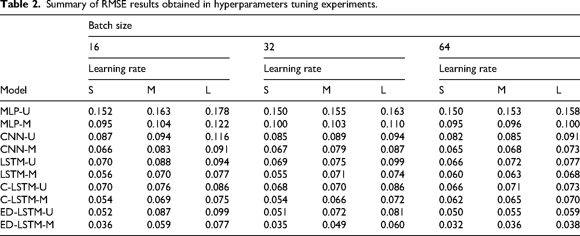
Results in Table 2 shows a clear trend regarding the two studied hyperparameters. Smaller learning rates allowed to compute better (lower) RMSE values for all ANN models. It is well known that the leaning rate plays an important role optimization problem related to ANN training. Smaller learning rates help an smooth exploration of the loss landscape, escape from local minima, and more precisely convergence towards the optimal minimum. Smaller values of learning rate also allows a more gradual and stable training process, unlike larger learning rates that may lead the optimization to instability and oscillations. The resulting trained model has better generalization, since it is less likely to fit noise in the training data and more likely to capture underlying patterns that can improve forecasting accuracy on unseen data. This result has been confirmed in real world engineering and renewable energy prediction problems (Matrenin et al., 2020; Rangelov et al., 2023; Yang et al., 2024). Improvements using smaller learning rates were notable for the ED-LSTM-M, up to 53.3% using a batch size of 16, and reducing when using larger batch sizes.

Regarding the size of the batch used for training, results indicated that a slight improvement in prediction accuracy evaluated by the RMSE metric was obtained using larger batch sizes. Simpler models such as MLP and CNN, in both univarate and multivariate versions, did not improve significantly. LSTM and C-LSTM even worsened their RMSE values in some cases. ED-LSTM-M improved when using larger batches, up to 8.6% when using the most competitive (i.e., smaller) learning rate values.

In subsequent training and validation experiments, the studied ANN-based forecasting models were configured with the best hyperparameter values obtained in the analysis: learning rate between ${10}^{-6}$ and ${10}^{-5}$ and a batch size of 64.

Training experiments and results

The ANN models for wind power generation forecasting were trained using the Plant Load Factor values. These values are normalized in the SCADA reports, considering that the Plant Load Factor is calculated as the ratio of the power delivered by the wind plants to the total installed capacity. Using the normalized Plant Load Factor values instead of the actual delivered power offers three benefits: i) normalized values are less susceptible to training issues due to the prevalence of large values and large differences; ii) it simplifies the design of the studied ANN architectures, eliminating the need for an additional layer for input value normalization; and iii) enhances the robustness and scalability of the approach to accommodate planned variations in the installed wind power generation capacity within the country, as has been occurring in the last ten years.

Training experiments were executed over the augmented dataset created through the application of the described sliding window technique. Starting with 635 blocks in the original input file of historical observations, a total of 40 752 training blocks were generated through data augmentation.

Although training experiments were initially set to execute for 100 epochs, most variations of the studied ANNs achieved highly competitive RMSE results in 40–50 epochs, stagnating later. Training experiments demanded around 10 minutes to complete on a computing node of the Cluster-UY platform featuring a Tesla P100 GPU.

Table 3 reports the median values of the RMSE and MAE metrics obtained in training experiments for the studied ANN-based forecasting models. Results are reported for hours 24 (first day), 48 (second day), and 60, as the predictions tended to degrade afterwards.

Table 3.

Median values of the RMSE, MAPE, and MAE metrics obtained in training experiments for the studied ANN models.

Model	RMSE
	Median	Hour 12	Hour 36	Hour 60
MLP-U	0.251	0.128	0.161	0.282
MLP-M	0.183	0.092	0.135	0.201
CNN-U	0.156	0.091	0.140	0.203
CNN-M	0.103	0.060	0.115	0.166
LSTM-U	0.129	0.087	0.107	0.198
LSTM-M	0.079	0.061	0.082	0.151
C-LSTM-U	0.134	0.072	0.107	0.178
C-LSTM-M	0.094	0.063	0.100	0.125
ED-LSTM-U	0.101	0.058	0.090	0.131
ED-LSTM-M	0.072	0.039	0.068	0.109

Model	MAE
	Median	Hour 12	Hour 36	Hour 60
MLP-U	0.149	0.082	0.127	0.182
MLP-M	0.089	0.061	0.105	0.158
CNN-U	0.131	0.076	0.116	0.159
CNN-M	0.080	0.054	0.079	0.141
LSTM-U	0.107	0.070	0.098	0.148
LSTM-M	0.067	0.050	0.076	0.101
C-LSTM-U	0.105	0.065	0.092	0.147
C-LSTM-M	0.072	0.054	0.079	0.100
ED-LSTM-U	0.096	0.042	0.081	0.122
ED-LSTM-M	0.056	0.031	0.053	0.099

Model	MAPE
	Median	Hour 12	Hour 36	Hour 60
MLP-U	29.1%	17.5%	24.8%	35.0%
MLP-M	19.0%	13.3%	21.5%	25.9%
CNN-U	23.3%	16.0%	20.9%	32.6%
CNN-M	16.7%	10.9%	15.4%	29.8%
LSTM-U	21.6%	14.2%	20.3%	31.0%
LSTM-M	14.0%	10.5%	14.5%	22.9%
C-LSTM-U	21.4%	13.1%	19.0%	30.4%
C-LSTM-M	15.3%	11.0%	16.2%	22.3%
ED-LSTM-U	18.9%	8.9%	15.9%	24.6%
ED-LSTM-M	11.7%	6.4%	10.7%	19.7%

Results in Table 3 indicate a satisfactory level of accuracy in training experiments. Median RMSE values ranged from 0.251 for MPL-U to 0.072 for ED-LSTM-M. The evolution through the hours showed that RMSE values computed for the third day (hour 60) worsened from two to three times of the value computed for the first predicted day. Median RMSE values of the multivariate forecasting models were between 19.6% (for the C-LSTM architecture) to 28.9% (for the LSTM architecture). The computed RMSE values are considered accurate for a normalized variable with significant variability such as the Plant Load Factor.

A similar trend was observed for the median MAE values. The best result was computed by ED-LSTM-M with a median value of 0.056 and MLP-U computed the worst results, with a median MAE value of 0.149. Multivariate models improved the median MAE from 24.1% (for the MLP architecture) to 30.0% (for the C-LSTM architecture).

Figure 5 showcases the evolution of the loss function (RMSE) values during the 100 epochs performed in training experiments for each one of the studied ANN-based forecasting models, in their univariate variants.

Figure 5.

Evolution of the RMSE as loss function in training experiments for the univariate versions of the studied ANN-based models for wind power generation forecasting.

In turn, Figure 6 shows the evolution of the loss function values for multivariate variants of the studied ANN-based forecasting models during the 100 epochs performed in training experiments.

Figure 6.

Evolution of the RMSE as loss function in training experiments for the multivariate versions of the studied ANN-based models for wind power generation forecasting.

Regarding univariate models, MLP-U and CNN-U showed unable to properly reduce the loss function values beyond 20 and 40 epochs, respectively. LSTM-U and C-LSTM-U had a better evolution, but clearly stagnating after 50 epochs. ED-LSTM-U further reduced the loss function values.

The best results were computed using multivariate models. However, MLP-M was still unable to reduce the RMSE below 0.03. CNN-M and LSTM-M significantly improved over their univariate counterparts. C-LSTM improved significantly in the last 15 epochs and ED-LSTM-M computed the best results, yielding almost null RMSE in trining experiments after 65 epochs. Results clearly demonstrate the benefit os using the numerical estimates as covariate in multivariate models and the clear superiority of the hybrid ED-LSTM model in forecasting. The faster pattern of RMSE reduction indicate that the hybrid approach was able to take advantage of the encoder and the decoder for properly capturing the most relevant features on the input wind power generation data.

Validation experiments and results

The validation phase considered the final (fifth) year of wind power generation data, distinct from the training set, to prevent bias. The studied ANN-based forecasting methods were assessed taking into account four primary dimensions: i) evaluating the forecasting capabilities of the proposed ANN-based models without employing numerical estimations as covariates; ii) studying the accuracy enhancement when incorporating numerical estimations as covariates; iii) examining the forecasting accuracy within a 24-hour timeframe, crucial for constructing scenarios in stochastic optimization methods for smart grid planning and scheduling, and iv) analyzing the forecasting precision under various wind conditions (calm, normal, and windy days). The metric used for evaluation is MAE, to evaluate the absolute error of the generated forecasts.

Forecasting results for univariate models

Table 4 presents the MAE values obtained in validation experiments conducted on the univariate variants of the studied ANN-based forecasting models, where numerical estimations were not utilized as covariates. As for training experiments, MAE results are reported for hour 12, 36, and 60.

Table 4.

MAE and MAPE values obtained in validation experiments for univariate variants of the studied ANN models.

Model	MAE
	Median	Hour 12	Hour 36	Hour 60
MLP-U	0.191	0.128	0.189	0.240
CNN-U	0.162	0.119	0.160	0.215
LSTM-U	0.147	0.108	0.156	0.204
C-LSTM-U	0.135	0.106	0.149	0.197
ED-LSTM-U	0.124	0.093	0.128	0.159

Model	MAPE
	Median	Hour 12	Hour 36	Hour 60
MLP-U	38.6%	25.1%	37.3%	45.4%
CNN-U	32.7%	24.6%	32.1%	42.0%
LSTM-U	30.0%	23.0%	30.5%	40.6%
C-LSTM-U	26.2%	21.6%	28.7%	40.0%
ED-LSTM-U	24.4%	19.5%	24.2%	36.8%

Results in Table 4 indicate that the univariate variants of the studied ANN-based forecasting models had a diverse accuracy regarding the MAE metric. Simpler models such al MLP-U and CNN-U had median MAE values over 0.16 on the entire forecasting period, and over 0.21 on hour 60 and afterwards. LSTM-U and C-LSTM-U improved slightly the overall MAE values, and ED-LSTM-U computed the best results among univariate models, but with a median MAE over 0.12.

Validation of multivariate forecasting models

Table 5 presents the obtained MAE values in the multivariate.

Table 5.

MAE and MAPE values obtained in validation experiments for multivariate variants of the studied ANN models.

Model	MAE
	Median	Hour 12	Hour 36	Hour 60
MLP-M	0.147	0.134	0.149	0.170
CNN-M	0.124	0.102	0.126	0.158
LSTM-M	0.105	0.099	0.106	0.123
C-LSTM-M	0.087	0.079	0.091	0.108
ED-LSTM-M	0.072	0.056	0.070	0.093

Model	MAPE
	Median	Hour 12	Hour 36	Hour 60
MLP-M	31.7%	26.6%	30.0%	35.0%
CNN-M	26.1%	21.1%	26.4%	30.6%
LSTM-M	21.0%	20.4%	21.1%	24.7%
C-LSTM-M	19.3%	18.5%	18.6%	21.9%
ED-LSTM-M	14.9%	11.2%	14.7%	18.0%

Table 5 presents the MAE values obtained for hour 12, 36, and 60 in validation experiments conducted on the multivariate variants of the studied ANN-based forecasting models, including the numerical estimations as covariates.

Results in Table 4 demonstrate that the multivariate variants of the studied ANN-based forecasting models computed accurate values of the MAE metric. Except for the simplest models (MLP-M and CNN-M), the architectures than include an LSTM layer were able to properly forecast the wind power generation in the considered case study. The obtained results are competitive with previous reported forecasting in related works. LSTM-M had an overall median MAE of 0.105 and the hybrid models were below the 0.1 mark. ED-LSTM-M computed excellent results, with a median of 0.072 and values as low as 0.056 for hour 12. In turn, results did not worsen significantly for the last hours in the forecasting period, e.g. a MAE of 0.093 was obtained for hour 60. Figures 7 to 11 present a comparative analysis of the results obtained by univariate and multivariate models.

Figure 7.

Comparison of univariate and multivariate variants of the MLP model.

Figure 8.

Comparison of univariate and multivariate variants of the CNN model.

Figure 9.

Comparison of univariate and multivariate variants of the LSTM model.

Figure 10.

Comparison of univariate and multivariate variants of the C-LSTM model.

Figure 11.

Comparison of univariate and multivariate variants of the ED-LSTM model.

Results in Tables 4 and 5 and Figures 7 to 11 show the superiority of multivariate models over univariate counterparts. Better MAE results were obtained except for early forecasts (up to hour 12) for MLP, CNN, and LSTM models. Average MAE results improved up to 0.052 for ED-LSTM, the best forecasting model when using numerical estimations in the learning process as covariate in validation experiments. Unlike previous results obtained for the prediction of wind power generation (Nesmachnow and Risso, 2025), the improvements on the MAE metric increased for advanced hours in the forecasting horizon, up to 0.089 for the C-LSTM model for hour 60.

These findings highlight the effectiveness of incorporating numerical estimations as covariates in the learning procedure. The results obtained align with those documented in relevant literature concerning analogous forecasting challenges. The MAE score of 0.093 achieved with the ED-LSTM-M model represents a notably strong outcome for predicting winf power generation 60 hours ahead. Furthermore, the median MAE of 0.072 represents a remarkable level of precision in predicting wind power generation for a dataset characterized by significant variability.

Table 6 reports the the median RMSE computed for the best forecasting model (ED-LSTM-M) and the real data for each hour in the forecasting horizon, in the validation experiments.

Table 6.

Median RMSE values of the real value of wind power generation and the forecast using the ED-LSTM model ( $\overline{\text{RMSE}}$ ) for each hour (H) in the forecasting horizon in the validation experiments.

H	$\overline{\text{RMSE}}$	H	$\overline{\text{RMSE}}$	H	$\overline{\text{RMSE}}$	H	$\overline{\text{RMSE}}$	H	$\overline{\text{RMSE}}$	H	$\overline{\text{RMSE}}$
1	0.056	2	0.098	3	0.112	4	0.107	5	0.108	6	0.104
7	0.100	8	0.100	9	0.095	10	0.086	11	0.080	12	0.079
13	0.086	14	0.092	15	0.101	16	0.104	17	0.108	18	0.105
19	0.112	20	0.122	21	0.123	22	0.126	23	0.125	24	0.111
25	0.104	26	0.106	27	0.107	28	0.104	29	0.109	30	0.119
31	0.126	32	0.123	33	0.118	34	0.115	35	0.124	36	0.133
37	0.131	38	0.126	39	0.128	40	0.116	41	0.115	42	0.111
43	0.109	44	0.111	45	0.112	46	0.113	47	0.119	48	0.120
49	0.120	50	0.132	51	0.131	52	0.122	53	0.122	54	0.112
55	0.113	56	0.122	57	0.116	58	0.119	59	0.123	60	0.125
61	0.121	62	0.121	63	0.125	64	0.123	65	0.119	66	0.121
67	0.129	68	0.138	69	0.144	70	0.157	71	0.165	72	0.165

Results in Table 6 highlight the high accuracy of the predictions by ED-LSTM-M. Median RMSE values were accurate considering previously reported results in related works. Although values increased for the latter hours in the forecasting horizon, even the forecasts for three days ahead had a reasonable accuracy, below 16.5%.

Table 7 presents the differences between the forecasts of the best model (ED-LSTM-M) and real data for each hour in the forecasting horizon, in validation experiments. Results follow the commented behaviour for median RMSE values. The worst median difference was 3.19 $\times$ 10⁻² at hour 52. ED-LSTM-M also demonstrated a high robustness, since errors slightly worsened when advancing in the hours of the forecasting period. Like the other studied models, a poorer performance was shown beyond hour 64, indicating that the accumulation of errors poses challenges for accurate forecasting. However, even for three days ahead, the differences were below 10%. To enhance accuracy for the later hours within the forecasting horizon, targeted adjustments need to be implemented in the ANN-based forecasting models. Nevertheless, this limitation does not detract the usefulness of the proposed methodology, primarily due to LSTM models generated precise results. Moreover, by applying the computed forecasts within an earlier time frame within the horizon (e.g., at hours 24 or 48) and subsequently updating the model, it is possible to mitigate the decline in accuracy for the later hours.

Table 7.

Median of the differences between the real value of wind power generation and the forecast using the ED-LSTM model ( $\stackrel{\sim }{{\mathrm{\Delta }}_W}$ ) for each hour in the forecasting horizon in the validation experiments.

H	$\stackrel{\sim }{{\mathrm{\Delta }}_W}$	H	$\stackrel{\sim }{{\mathrm{\Delta }}_W}$	H	$\stackrel{\sim }{{\mathrm{\Delta }}_W}$	H	$\stackrel{\sim }{{\mathrm{\Delta }}_W}$	H	$\stackrel{\sim }{{\mathrm{\Delta }}_W}$	H	$\stackrel{\sim }{{\mathrm{\Delta }}_W}$
1	−2.45 $\times$ 10−4	2	−1.15 $\times$ 10−2	3	−1.43 $\times$ 10−2	4	−2.06 $\times$ 10−2	5	−7.44 $\times$ 10−3	6	−8.37 $\times$ 10−3
7	−7.40 $\times$ 10−3	8	−2.91 $\times$ 10−3	9	−1.52 $\times$ 10−2	10	−1.51 $\times$ 10−2	11	−9.75 $\times$ 10−3	12	−7.19 $\times$ 10−3
13	7.37 $\times$ 10−3	14	1.05 $\times$ 10−2	15	1.73 $\times$ 10−3	16	2.59 $\times$ 10−4	17	2.98 $\times$ 10−3	18	2.83 $\times$ 10−3
19	8.61 $\times$ 10−3	20	1.24 $\times$ 10−2	21	3.31 $\times$ 10−3	22	3.44 $\times$ 10−3	23	5.01 $\times$ 10−3	24	1.32 $\times$ 10−2
25	2.31 $\times$ 10−2	26	4.97 $\times$ 10−3	27	4.74 $\times$ 10−3	28	3.11 $\times$ 10−4	29	−2.36 $\times$ 10−4	30	−1.30 $\times$ 10−3
31	-4.29 $\times$ 10−3	32	−6.87 $\times$ 10−3	33	6.94 $\times$ 10−3	34	3.91 $\times$ 10−3	35	3.74 $\times$ 10−3	36	−4.48 $\times$ 10−3
37	−6.02 $\times$ 10−4	38	−3.43 $\times$ 10−4	39	8.11 $\times$ 10−3	40	2.67 $\times$ 10−4	41	−1.74 $\times$ 10−3	42	−1.75 $\times$ 10−3
43	9.51 $\times$ 10−3	44	1.37 $\times$ 10−2	45	1.36 $\times$ 10−2	46	1.01 $\times$ 10−2	47	−4.78 $\times$ 10−3	48	−1.74 $\times$ 10−2
49	−3.01 $\times$ 10−2	50	−2.88 $\times$ 10−2	51	−3.02 $\times$ 10−2	52	−3.19 $\times$ 10−2	53	-1.07 $\times$ 10−2	54	−4.19 $\times$ 10−3
55	3.03 $\times$ 10−3	56	−3.81 $\times$ 10−3	57	−9.17 $\times$ 10−3	58	−8.77 $\times$ 10−3	59	9.62 $\times$ 10−3	60	2.20 $\times$ 10−2
61	2.29 $\times$ 10−2	62	2.05 $\times$ 10−2	63	2.24 $\times$ 10−2	64	6.28 $\times$ 10−3	65	4.64 $\times$ 10−4	66	8.45 $\times$ 10−3
67	9.92 $\times$ 10−3	68	1.74 $\times$ 10−2	69	1.20 $\times$ 10−2	70	1.80 $\times$ 10−2	71	4.49 $\times$ 10−3	72	−7.76 $\times$ 10−3

The boxplots in Figure 12 presents the statistical information about the differences between the real and the forecasted wind power generation using model ED-LSTM-M. Values in each boxplot correspond to the distributions of results obtained in 408 predictions performed for each hour in the validation experiments.

Figure 12.

Boxplots the differences between the real and the forecasted wind power generation using model ED-LSTM-M for each hour, in the validation experiments.

Values in Figure 12 indicate that the differences between the real and the forecasted wind power generation were reduced. The boxplot heights, that represent the interquartile range of the distributions were between 0.05 in the first predicted hours and 0.17 at the end of the forecasting period. These results confirm a high accuracy on the predictions, especially in the short-term. In turn, the distribution of wind power generation forecasts has just a few number of outliers, most of them at hours 36 to 40 and at the end of the forecasting horizon. Outliers are caused by non predictable phenomena related to wind availability, including sudden changes in wind direction and speed, turbulence, atmospheric instabilities leading to unpredictable wind behaviour, eddies and vortices that can affect wind patterns, among other situations. Overall, the boxplots confirm the high quality of the ED-LSTM-M forecasts.

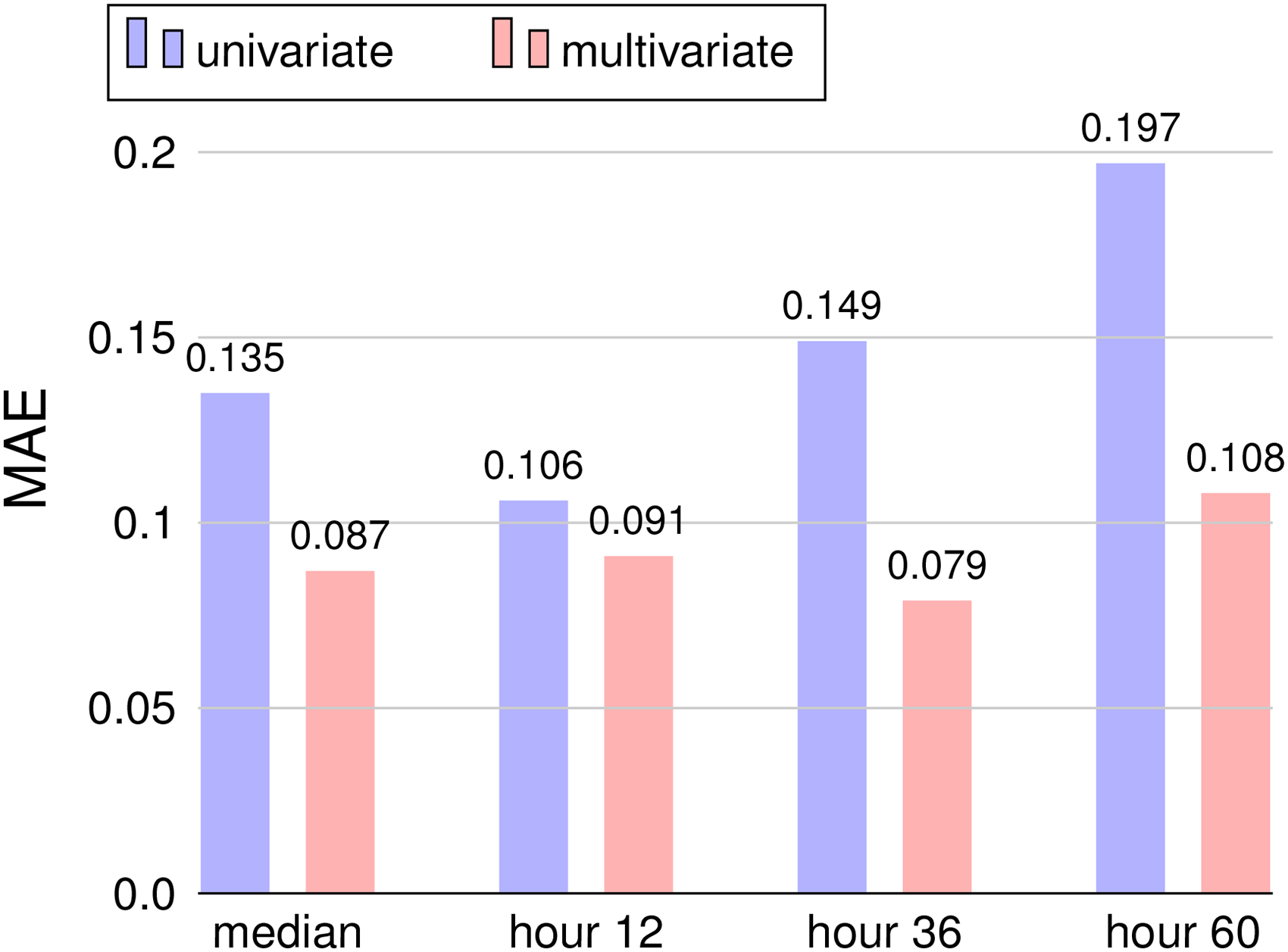
Figure 13 presents a graphical comparison of the main results obtained in the validation of the studied ANN-based forecasting methods, using a Kiviat diagram. The median values of RMSE, MAE, and MAE for 24 hours are reported and compared for each version of the studied method. Results clearly shows the accuracy (values closer to the centre of the diagram are better, as they represent lower RMSE and MAE values) of multivariate versions of the studied methods, its superiority over univariate versions, and also the high accuracy of ED-LSTM-M for both overall and 24-hour predictions.

Figure 13.

Kiviat diagram: average RMSE, average MAE, and 24-hour MAE for the compared ANN-based forecasting methods.

Analysis of the NPV parameter

Table 8 reports the analysis of MAE and MAPE metrics for the multivariate methods for different values of the NPV parameter (24, 48, and 72 hours). The average execution times are also reported, to analyze the trade-off between forecasting accuracy and training time.

Table 8.

Median MAE and MAPE values computed in experiments using different values of the NPV parameter, and average execution time for the studied multivariate ANN models.

Model	MAE
	NPV $=$ 24	NPV $=$ 48	NPV $=$ 72	Time
MLP-M	0.162	0.158	0.147	7.8 m
CNN-M	0.149	0.140	0.124	8.0 m
LSTM-M	0.141	0.128	0.105	10.0 m
C-LSTM-M	0.119	0.104	0.087	11.2 m
ED-LSTM-M	0.094	0.087	0.072	11.6 m

Model	MAPE
	NPV $=$ 24	NPV $=$ 48	NPV $=$ 72	Time
MLP-M	31.7%	31.0%	28.6%	8.1 m
CNN-M	31.0%	29.2%	24.0%	8.7 m
LSTM-M	29.1%	25.7%	20.3%	10.5 m
C-LSTM-M	23.9%	22.5%	16.9%	12.0 m
ED-LSTM-M	19.7%	18.8%	13.6%	12.6 m

Results in Table 8 indicate that improvements of up to 23% for MAE and up to 31% for MAPE were obtained when using NPV $=$ 72, compared to using NPV $=$ 24. The average MAE and MAPE values reduced for all models when including more historical data in training. Generally, as the number of previous observations increased, a trend of decreasing MAE and MAPE values was detected, suggesting that incorporating more historical data improves the predictive capabilities of the models. The increase in training execution time with more complex models or larger datasets is also evident in the provided data. Nevertheless, the impact on execution time is not critical, as the trade-off between higher accuracy and longer execution time is reasonable and affordable for the practical implementation of the studied models.

Predictions of wind power generation for different wind conditions

Table 9 presents the median values of the MAE and MAPE metrics obtained by the multivariate versions of the compared ANN-based forecasting models in validation experiments, considering periods with different wind conditions (calm, normal, and windy). The considered wind conditions are calm, normal, and windy, based on the speed of the wind according to the modern Beaufort wind scale, a common way to measure wind speed. The calm category includes calm, light air, and light breeze in the Beaufort scale, with a wind speed ranging between 1 and 11 km/h; the normal category includes gentle breeze, moderate breeze, and fresh breeze in the Beaufort scale, with a wind speed ranging between 12 and 38 km/h; and the windy category includes from strong breeze to speedier wind conditions, over 39 km/h.

Table 9.

Median MAE and MAPE values obtained for the multivariate versions of the studied ANN forecasting models in validation experiments, for days with different wind conditions.

Model	median MAE
	Overall	Calm	Normal	Windy
MLP-M	0.147	0.126	0.170	0.212
CNN-M	0.124	0.109	0.152	0.187
LSTM-M	0.115	0.095	0.159	0.200
C-LSTM-M	0.097	0.066	0.110	0.123
ED-LSTM-M	0.072	0.022	0.070	0.099

Model	Median MAPE
	Overall	Calm	Normal	Windy
MLP-M	31.1%	24.9%	32.9%	38.2%
CNN-M	27.0%	22.8%	30.6%	34.6%
LSTM-M	22.9%	21.0%	32.0%	39.5%
C-LSTM-M	20.7%	11.8%	23.1%	25.3%
ED-LSTM-M	16.4%	4.1%	15.3%	20.7%

Results in Table 9 show that very accurate predictions were generated for calm wind conditions using LSTM-M, C-LSTM-M, and ED-LSTM-M, with a median MAE below 0.1 for all methods and a minimum of 0.022 for the ED-LSTM-M model. The previously commented finding suggests that calm days were easy to predict, mainly because high variations in wind speed, thus in wind power generation, are not present. However, in calm days the studied ANN-based forecasting methods also suffer from the well-know phenomena of overfitting to very low and null values (i.e., a constant prediction of zero or near zero has a very reduced MAE value), that must be taken into account.

Normal and windy days were harder for predictions and only ED-LSTM-M computed median MAE values below 0.100. In any case, the hybrid C-LSTM-M architecture also computed accurate predictions, with median MAE of 0.110 for normal days and 0.123 for windy days. These results align with forecasting results reported for other case studies in the world.

Computational efficiency

Table 10 reports the average (avg.) and standard deviation ( $\sigma$ ) of the execution times required for each studied ANN-based forecasting method in training and validation/inference experiments.

Table 10.

Average and standard deviation of execution times in training and validation experiments for the studied ANN models.

Model	Eecution Time (avg.  $\pm$   $\sigma$ )
	Training	Validation/Inference
MLP-U	7.8  $\pm$  0.4 m	2.0  $\pm$  0.1 s
CNN-U	8.0  $\pm$  0.6 m	2.3  $\pm$  0.1 s
LSTM-U	10.0  $\pm$  0.5 m	2.7  $\pm$  0.2 s
C-LSTM-U	11.2  $\pm$  1.0 m	2.6  $\pm$  0.2 s
ED-LSTM-U	11.6  $\pm$  0.9 m	2.7  $\pm$  0.2 s

Model	Execution Time (avg.  $\pm$   $\sigma$ )
	Training	Validation/Inference
MLP-M	8.1  $\pm$  0.4 m	2.0  $\pm$  0.1 s
CNN-M	8.7  $\pm$  0.6 m	2.2  $\pm$  0.2 s
LSTM-M	10.5  $\pm$  0.6 m	2.7  $\pm$  0.2 s
C-LSTM-M	12.0  $\pm$  1.2 m	2.7  $\pm$  0.2 s
ED-LSTM-M	12.6  $\pm$  1.0 m	2.8  $\pm$  0.2 s

Training times ranged from 7.8 to 12.6 minutes (univariate models) and from 8.1 to 12.6 minutes (mutivariate models). C-LSTM-M and ED-LSTM-M had the longest training times (up to 50% longer than the simplest models), showing that hybrid architectures required more computational resources due to its more complex training process. Including the numerical estimations as covariant resulted in about one additional minute (between 8% and 12% more) required for the training process. Lower execution times are generally desirable, especially for scenarios where computational efficiency is crucial. However, longer training times might be acceptable if they result in better model performance, as demonstrated in the reported results.

Validation/inference execution times were significantly lower, from 2.0 to 2.8 seconds for both univariate and mutivariate models. Differences between models were not significant, as shown by the standard deviation values. The execution times for validation/inference indicate that the studied ANN are relatively fast and suited for integration in real-time applications. In particular, they can be included in current operation and management tools for the smart grid in Uruguay. The developed models provide real-time responsiveness to support quick decision-making based on incoming data and are useful for interactive applications where immediate feedback or predictions are needed.

Even though execution times are often influenced by the complexity of the ANN architecture, the fast validation/inference times strike a proper balance between accuracy, models complexity, and computational efficiency. Models with additional layers did not increase significantly the execution times, providing flexibility and a good trade-off between speed and accuracy.

The trade-offs between computational cost and model effectiveness are reasonable for the best performing model (ED-LSTM-M) that allowed to improve the forecasting results just requiring between three and four additional minutes for training and lees than a second additional seconds for inference.

Examples of predicted time series of wind power generation

Figures 14 and 15 present two examples of the time series of wind power generation predicted by ED-LSTM-M. The predicted time series correspond to representative periods in the validation dataset (1000 hours each), with different wind conditions.

Figure 14.

Examples of representative wind power generation forecasts by model ED-LSTM-M (orange curve) and real wind power generation values (blue curve): period between April 1, 2021 and June 23, 2021.

Figure 15.

Examples of representative wind power generation forecasts by model ED-LSTM-M (orange curve) and real wind power generation values (blue curve): period between July 1, 2021 and September 22, 2021.

Figure 14 corresponds to wind power generation values between July 1, 2021 and September 22, 2021 and the graphic Figure 15 corresponds to wind power generation values in the period from April 1, 2021 to June 23, 2021. Both figures show accurate results, with the predicted time series of wind power generation values closely following the real values. An excellent prediction pattern is shown in Figure 14 (autumn 2021), with very minor deviations from the actual wind power generation values in the whole period. When wind conditions are highly variable, such as in Figure 15 (winter of 2021), the time series is slightly harder to follow accurately. Nevertheless, the ED-LSTM-M model computed precise values and followed the tendencies all along the reported period. The efficacy of using an hybrid ANN architecture including an encoder-decoder is shown in the comparison between Figure 16 (wind power generation predictions using LSTM-M) and Figure 17 (wind power generation predictions using ED-LSTM-M).

Figure 16.

Examples of representative wind power generation forecasts by model LSTM-M (orange curve) and real wind power generation values (blue curve): period between April 1, 2021 and June 23, 2021.

Figure 17.

Examples of representative wind power generation forecasts by model ED-LSTM-M (orange curve) and real wind power generation values (blue curve): period between April 1, 2021 and June 23, 2021.

Results reveal that the ED-LSTM-M model excels in capturing the dynamics of the time series, notably diminishing errors compared to the standard LSTM-M model. This trend is particularly evident in regions with unexpected variations on wind power generation. Two clear periods shown in the reported graphics with significant improvements of the ED-LSTM-M over the LSTM-M forecasts are from hour 250 to 325 (moderate wind conditions, Plant Load Factor values between 0.2 and 0.4), and from hour 720 to hour 780 (high wind conditions, Plant Load Factor values over 0.5). Leveraging the encoder-decoder layers, the ED-LSTM model adeptly adjusts its outputs to accommodate unforeseen fluctuations in wind power generation values. Findings underscore the remarkable predictive accuracy achieved by the hybrid ED-LSTM neural network approach, effectively capturing temporal patterns within the time series data with minimal deviations from the observed wind power generation values.

The applied hybrid model combining ED layers with a baseline ANN architecture is also an useful option, also to improve the predictive capabilities of other forecasting models, such as MLP, GRU, BiLSTM, etc. The main contributions of including the ED components are related to process input sequences and generate output sequences of varying lengths, providing flexibility in forecasting tasks with different historical data and prediction horizons. In turn, the ED components provide support for capturing long-range dependencies, taking advantage of enhanced feature extraction provided by the encoder, allowing learning complex patterns and relationships in the data. All this advantages result in enhanced generalization capabilities of the hybrid model. Considering the modular design of the developed code, the implementation of new hybrid models is rather easy. The empirical study of different hybrid models is proposed as one of the main research lines for future work.

Conclusions and future work

The article discussed the development and application of ANN-based methodologies to predict wind power generation at a national scale in Uruguay. The study centred around analyzing and predicting the actual time series data of wind power generation in Uruguay during the period spanning from 2018 to 2022.

Ten ANN-based forecasting models were examined: MLP, CNN, LSTM, C-LSTM, and ED-LSTM architectures in both univariate and multivariate versions, including additional data source from numerical estimates as covariant in the learning process. The ED layers were integrated into LSTM as it was the best performing model among the simpler architectures. The combination of ED with other simple models was not studied, to put a specific focus on the most accurate models. However, the modular and flexible design of the developed ANNs makes it easy to integrate and analyze new hybrid new models. To enhance the training process of the studied ANN architectures, specialized methods for data preprocessing and augmentation were implemented, and a variety of ANN architectures were assessed to determine their effectiveness in forecasting.

The primary outcomes of the experimental study showed that the multivariate version of the ED-LSTM technique yielded the most favourable results, surpassing the performance of the other models significantly. The obtained results were RMSE 0.12, MAE 0.09, and MAPE 14.9%. Overall, integrating numerical estimations as covariates into the training model led to an average 5% enhancement in median MAE results across all models. Statistical analysis verified the robustness of the results, as evidenced by compact boxplots when evaluating the results distributions between the predicted and the actual wind power generation values. Furthermore, the study revealed that forecasting precision varies with different wind conditions.

The ED-LSTM-M method exhibited promising predictive accuracy, obtaining a median MAE of 0.056 in training experiments and an overall median MAE of 0.090 in validation, a result that exceeded the performance of alternative ANN architectures. In particular, excellent results were computed by ED-LSTM-M for calm wind conditions, with a median MAE of 0.022, whereas windy days were significantly harder for predictions, as the accuracy declined up to 0.099 of median MAE.

The generated forecasts are very valuable and have significant implications for potential integration into planning and scheduling processes, aiming to elevate the overall service quality of the electricity grid. As a relevant application, the forecasts generated using ED-LSTM-M are applicable to create different scenarios for the validation of a stochastic optimization to fit energy bands, considering a given threshold for off-band energy.

The main lines for future work include exploring alternative ANN architectures for time series forecasting, such as Bidirectional LSTM and Gated Recurrent Units, to expand the scope of the study. Also, future work should analyze more complex techniques to bolster prediction accuracy in both the medium to long term and on days with high peaks in wind power generation values, where the studied ANN-based predictors yielded subpar results. The study of hybrid models combining ED with MLP, GRU, BILSTM is also a promising research line for future work, especially to broad the scope of ANN models. In this regard, the future research should focus on determining the adaptability of hybrid models to better capture fluctuant and difficult-to-predict situations regarding the availability of the wind resource. Finally, the viability of integrating the top-performing models to create scenarios for real-time stochastic models of short-term and medium-term renewable power generation operation is also proposed, to leverage potent data-driven methodologies to facilitate decision-making and operational activities within the electric smart grid.