Sage Journals: Discover world-class research

Abstract

Forecast models for wind speed and wind turbine power generation are valuable support tools for operators of Control Energy Center. In this work, a year of daily energy output of a wind turbine is analyzed. The original time series was separated into a high-power sample and a low-power sample. High-power sample has a seasonal pattern while low-power sample does not. Afterward, a sARIMA model was produced for high-power sample forecast, with a good performance, while for low-power sample any ARIMA model defeated persistence model; thus, a couple of nonlinear autoregressive artificial neural networks are proposed. Mean absolute error and mean square error are reported and demonstrate that the sARIMA model can predict satisfactorily high-power sample, even with limited data, while to forecast low-power sample, it is necessary to use a neural networks approach and all data available to produce accurate forecasts. In each case, a normalized comparison with persistence model is also reported. Finally, a method which uses previous data of daily output energy and forecasted future wind speed values from a numeric weather prediction model is presented to objectively identify whether the current time is in a high-power or low-power regime to choose the ad hoc daily output energy forecast model.

Keywords

Daily wind output power sARIMA artificial neural network one-step-ahead forecasting weather research forecast model

Introduction

Renewable energies have become a common alternative to generate electric power and have been established an important subject of governments’ development schemes. In Garcia-Heller et al.¹ government development schemes of Latin American Countries were analyzed. In all of those schemes, scenarios for year 2025, in which renewable energies should cover from 15% to 25% of total electrical demand, are presented. In each of the four evaluated Country development schemes, wind energy is considered among other renewable sources.

In these days, several scientific manuscripts focused in one or more of the many issues regarding wind speed and wind power analyses to increase the confidence and improve operative characteristics of wind power technologies are easily found. However, one of the aspects that is still an obstacle to achieve a deeper penetration of these technologies in power market is the intermittent behavior of wind speed.² Thus, forecast models (FMs) for wind speed and wind turbine power generation are valuable support tools for operators of Control Energy Center of power utility.³

Registering output power of a wind turbine (OPWT) has proved to be highly dependent on wind speed over other meteorological variables as air temperature and atmospheric pressure⁴; nevertheless, it also has some dependence on residual inertial momentum of blades and power loses due to complementary equipment load and energy conversion.⁵

To predict wind power is important to understand that many issues affect it, for instance, Stathopoulos et al.⁶ tested two approaches to forecast wind power: the first one uses historical hourly data of OPWT to obtain the forecast for future values of OPWT; the second one uses a database of wind speed to forecast future wind speed and then uses this result to calculate the wind power applying the turbine power curve from provider. It was concluded that for the data utilized, it was slightly better the first approach.

In Murugan et al.,⁵ the performance after 10 years of operation of three wind turbines was reported. The turbines were operating in a wind farm at different heights from the ground. Researchers only presented theoretical ideal (analytical formulae) and actual ideal wind power (power curve) as a comparison to the actual OPWT. Calculated power was different from observations in all cases, which means that using the original power curve to calculate output power become less accurate after long term operation. In Goretti et al.,⁷ it was proved and concluded that actual power curve of a brand-new wind turbine may be different to power curve of provider; hence, actual OPWT can be significantly different from the originally expected one.

To select the approach to predict wind turbine, it is important to clarify that every case of study has its own characteristics and goals. In Nagaraja et al.,⁸ the authors made a review of approaches to forecast separately wind speed/power, electrical load, and energy prices. It was found that for each variable, artificial intelligence, fuzzy theory, regression methods, numeric weather prediction (NWP), and statistical methods were employed. However, the characteristics of each case of study were not clarified. Some other approaches may consider less common scopes according to each case criteria, for example, in Nguyen and Metzger,⁹ the goal was to have monthly averaged wind speed forecast to improve wind turbine performance by controlling rotor speed in advance, while authors focused in theoretical single horizontal wind turbines to be placed in urban and suburban areas. Nevertheless, it is highly recommended to have at least hourly, or even more dense data samples of observations; thus, performance of hourly forecasts of wind power could be improved;^3,5,10 nevertheless, sometimes available data do not have these features or the research goal is to analyze daily output energy (DOE).^11,12

In this work, an analysis of a yearlong sample of DOE of a Skystream Wind Turbine is presented. After analyzing the original time series, it was found that it may be composed by two populations corresponding to year seasons. The main contributions of this work to the state of the art are a sARIMA model and a non-autoregressive (NAR) model to forecast DOE for the next day of a wind turbine. The proposed models are suitable for different sections of the original data. The results showed that this annual time series can be separated into shorter time series corresponding to different power regimes and therefore, they need ad hoc forecasting models. Finally, a methodology to identify the current wind power regime is presented which will indicate the FM to select. In this method, it is proposed to use the DOE average of the previous days and the wind speed forecast for the following 24 h obtained through the weather research forecast (WRF) model. A list of all abbreviations is given in Table 1.

Table 1.

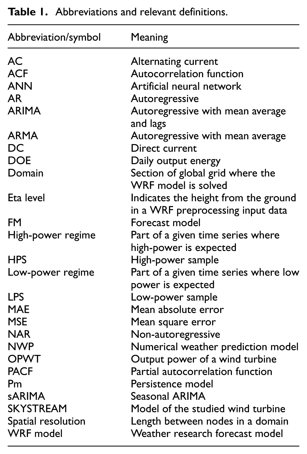
Abbreviations and relevant definitions.

Abbreviation/symbol	Meaning
AC	Alternating current
ACF	Autocorrelation function
ANN	Artificial neural network
AR	Autoregressive
ARIMA	Autoregressive with mean average and lags
ARMA	Autoregressive with mean average
DC	Direct current
DOE	Daily output energy
Domain	Section of global grid where the WRF model is solved
Eta level	Indicates the height from the ground in a WRF preprocessing input data
FM	Forecast model
High-power regime	Part of a given time series where high-power is expected
HPS	High-power sample
Low-power regime	Part of a given time series where low power is expected
LPS	Low-power sample
MAE	Mean absolute error
MSE	Mean square error
NAR	Non-autoregressive
NWP	Numerical weather prediction model
OPWT	Output power of a wind turbine
PACF	Partial autocorrelation function
Pm	Persistence model
sARIMA	Seasonal ARIMA
SKYSTREAM	Model of the studied wind turbine
Spatial resolution	Length between nodes in a domain
WRF model	Weather research forecast model

Forecast models

In order to propose any FM, it is important to identify the main characteristics of the prevailing models according to the literature. There are many time series prediction models, however, to identify the current FM to predict wind speed and wind turbine power output in the literature is essential, for a deeper search retrieve to references.^8,13,14 Nevertheless, probabilistic, statistical, and artificial intelligence approaches can be considered as the most frequently used.⁸ A concise description of most common models is presented in the following sections.

Forecast horizons

To understand the meaning of the forecast horizons and their dependence on historical data, Veit et al.¹⁵ can be revised in which a clear definition is established: “the prediction horizons are the number of points in the future that the algorithm will predict.” In addition, granularity is defined as the frequency of data. The granularity of forecast cannot be higher than the original data’s. If a time series has data every t hours, the nearest prediction will be t hours in the future and all other predicted points will appear with intervals of t hours.¹⁵

Generally, prediction horizons can be classified as: very-short-term forecast, when predicting up to 6-step-forward; short-term, which reaches up to 72-step-forward; and mid- and long-term forecast, when predicting over 72-step-forward.

In our case study, the time series of historical data has a frequency of one data per day, in which each of these data indicates the total energy produced in a day. So, the models for this case study make a short-term prediction because it is a forecast one-step ahead.

Persistence

Along the years, persistence model (Pm) has been chosen as a model to forecast intermittent phenomena related to meteorological variables. This is due to its simplicity, since it consists in considering the last observed value (t – 1) as the value that will present at time t + 1. Pm is also very accurate, specially, in short horizons forecasts.⁹

In addition, Pm is widely used as a comparison in order to validate any proposed FM related to highly random phenomena, as seen in several works.^{4,8,9,15–22}

For very short and short-term forecasts, persistence is the most used due to its simplicity as benchmark since it does not need even the calculation of coefficients. We can highlight the work of Koçak,²³ where the authors use the persistence model as a benchmark to compare hourly energy forecast models of a wind turbine with many forecast horizons (up to 24-step-forward).

Due to the characteristics of our time series, in which the energy production of a wind turbine is quantified, in which its resolution allows only one data per day to be considered, persistence can be used as a reference model that can allow an adequate comparison for our one-step-forward models.

ARIMA models

Basic statistical models to forecast time series can be (1) autoregressive (AR), (2) autoregressive with moving average (ARMA), and (3) autoregressive integrated with moving average (ARIMA), among several variations of them. These models are quite accurate to forecast wind speed and power of wind turbines.^24,25

Non-seasonal ARIMA models are represented as ARIMA (p, d, q), and to select all the coefficients, usually Box–Jenkins methodology is used.²⁶ In ARIMA models, p is the order of the autoregressive part, d is the order of the derivative, and q indicates the degree of the moving average. Linear representation is condensed in equation (1) as follows²⁷

y_{t} = \sum_{i = 1}^{p} ϕ_{i} y_{t - i} + \sum_{i = 1}^{q} θ_{j} y_{t - j} + ε_{t}

(1)

ARIMA models that have seasonal features are known as sARIMA and consist in the addition of more terms to the equation of above. The condensed form is sARIMA (p, d, q) (P, D, Q)_s. The P, D, and Q represent the same as in ARIMA, while s indicates the number of lags.²⁷

ANN

Artificial neural network (ANN) is numerical model that has some similar characteristics to human neurons in the way they share information. Information enters to the ANN through the first layer of neurons and then it passes into the inner layers (hidden layers) that can be one or multiple layers of neurons which spread the “weight” of the received inputs. Finally, the output layer, which consists in a single neuron layer, delivers the model’s result.²⁷ In Figure 1, a conceptual scheme of a nonlinear autoregressive (NAR) neural network is presented.²⁸

Figure 1.

Scheme of a non-autoregressive neural network.²⁸

Neural networks use a training phase that requires a part of the series, this enables to correct the initial weight distribution in the hidden layers, other percentage of observations is used to validate the model, and finally the remaining data are used to test the forecast.²⁹ An 80-10-10 percentage share of data is commonly use, respectively for each phase.

NWP models

NWP models are widely utilized in mesoscale approaches of wind speed predictions. Generally, these models are proposed to characterize places where there are no direct measurements of meteorological stations.^30,31 In the case of using NWP models to predict wind power, some approaches include those in which operational wind farms performance can be predicted or those in which the goal is to project power generation in a mid-term forecast with sufficiently good level of accuracy.³²

Hybrid models

It is common to find case studies in which researchers decide to apply hybrid forecasting model with a wide variety of configurations, however, hybrid models can be roughly defined as those that utilize different techniques or approaches in order to improve a given model, whether statistical or ANN.^3,31 Hybrid models can also include results obtained by NWP models.³²

Forecast validation

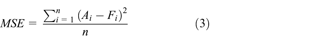
In each case, it is mandatory to analyze the certainty or accuracy of the models. To accomplish this, it can be computed the mean absolute error (MAE) and the mean square error (MSE). Their formulae are as follows²⁵

MAE = \frac{\sum_{i = 1}^{n} | A_{i} - F_{i} |}{n}

(2)

MSE = \frac{\sum_{i = 1}^{n} {(A_{i} - F_{i})}^{2}}{n}

(3)

Methodology

This section lists the activities that were conducted during this investigation and the order in which they appear in the manuscript.

The original time series is described by descriptive statistics:

Based on the results, it was decided to separate it into two time series: one with a high-power regime and another with a low power regime.

These time series were analyzed separately.

When analyzing the seasonality of the resulting HPS and LPS series, it is evident that the high-power series has a seasonal pattern, whereas the low power series does not.

Therefore, to predict the DOE energy a step forward, we obtained a sARIMA model with good error measurements. Considering the data features, it was concluded that this FM is suitable to predict DOE whenever high variability is detected.

For LPS an attempt was made to look for an ARIMA model, however, none of the ARIMA models achieved a better performance than persistence. Therefore, a NAR model was used for this part of the data.

Two approaches are proposed in the approach to use NAR, one in which only the LPS data are used to train the neural network, and another in which training is done with all the data of the original series.

Finally, a method to select between the FMs found is exposed. Based on the DOE average of the previous 15 days and the wind speed forecast obtained by WRF for the next 24 h, the current time regime can be identified, and thus, the ad hoc model can be selected.

In the following sections, the case study is described, and the separation of the time series according to the power regime is presented.

Case of study

In the presented case study, the performance of a Skystream wind turbine (SKYSTREAM) with the characteristics of Table 2 is analyzed.³³

Table 2.

Wind turbine characteristics.³⁴

Manufacturer/model	XZERES/Skystream 3.7
Max power	2.6 kW
Rated power	2.1 kW at 11 m/s
Weight	77 kg
Rotor diameter	3.72 m
Rotor RPM	350 r/min
Voltage	120 V, 1 phase, 60 Hz
Cut-in speed	3.2 m/s
Rated speed	11 m/s

The SKYSTREAM is placed in the city of Morelia in Michoacán, México, in the campus of the Universidad Michoacana of San Nicolás of Hidalgo Campus on the roof of Omega building facilities (Electrical Engineering Faculty accommodations) at the coordinates: $19.686935$ North, $- 101.204436$ East. The rotor is located at 18 m of height from the ground on the top of the roof, as shown in Figure 2.

Figure 2.

(a–d) Installed turbine Skystream 3.7. (e) Image from website of manufacturer.

The energy of the turbine is a direct current (DC) source that passes through a controller–inverter that convert it in alternating current (AC). Afterwards, it is connected directly to facilities’ main circuit that is an interconnected circuit that uses main energy network as backup supply. This turbine has a datalogger that register daily cumulative energy provided to the building, it has an interface where actual RPM of rotor and actual power produced can be observed, giving the possibility of register data in several formats. However, the automated acquisition routine of datalogger registers only daily energy; thus, the best yearly DOE dataset from those available was chosen.

Due to limitations of datalogger and data acquisition, DOE data between 2013 and 2016 were available. However, there are some lacks in data acquisition due to failure of operation or maintenance. Hence, a year with no missed data was analyzed. This dataset has the following features:

There are acceptable values of DOE in the first months of the year.

The mid-year months present lower power.

The last months of the year are again acceptable.

In Figure 3, the histogram of DOE is presented. It is easily observed that probability distribution fits the Weibull distribution function. In Table 3, descriptive statistics of original sample are also presented.

Figure 3.

Frequency histogram of DOE (2015).

Table 3.

Descriptive statistics of dataset of DOE.

Mean (kWh)	0.539
Mode (kWh)	0 (55 times)
Standard deviation (kWh)	0.7969
Maximum (kWh)	5.05
Minimum (kWh)	0
Total production of year (kWh)	216.76

DOE: daily output energy.

Box diagram of sample with outliers can be observed in Figure 4. Many values are possible outliers; however, due to the fact that probability distribution corresponds to Weibull distribution; there was no outliers analysis to this dataset.

Figure 4.

Box diagram of DOE (2015).

Before choosing the forecasting model, it is necessary to stabilize the mean and variance to try to identify the best model. In Figure 5, the results of this process are shown, where the new range of time series lies between −1 and 1. To stabilize this dataset, its third derivative was applied.

Figure 5.

Actual DOE and stabilized series on the variance.

Autocorrelation function (ACF) and partial autocorrelation function (PACF) of stabilized series were revised, in order to define whether to consider or not the lags to select an ARIMA model. Figure 6 shows both ACF and PACF. In (a) only the first lag appears as significant, while in (b) there is a group of some lags that may appear as significant; thus, ARIMA model must consider some lags in order to be more accurate.

Figure 6.

(a) ACF and (b) PACF of original stabilized series with a 5% of confidence level.

In the following section, further analyses are presented, including a seasonality test and the FMs proposed for these data.

Results

ARIMA and sARIMA models

Initially, a model for a whole year of power output of a wind turbine was proposed: 2015 (actual data, Figure 5) was considered. An 80-10-10 percentage share was utilized: 80% of observations to obtain the model’s coefficients, 10% for validation, and 10% to make the a-step-ahead forecast.

Several ARIMA models were tested from which histograms, ACF and PACF of residuals were obtained to select the one with the best performance. When results of forecasts and actual data were compared, it was found that none of the ARIMA models did accomplished to have an acceptable performance of the error tests (MAE and MSE). Because of the fact that wind power depends on meteorological variables, it was concluded that the poor performance of the originally tested ARIMA models had a straight relation with site’s weather characteristics.

Addressing more properly the original dataset in Figure 5 (black line), it was identified that these data may have two populations. In addition, there is some evidence that may indicate that these populations have a correlation with seasons and time of the year.

The first months as well as the last ones of the year have a higher variability than the one that show the months between April and August. From mid-autumn to the early spring, DOE reaches higher peaks, while the rest of the year appear to have lower ones. In Figure 7, a whole year of DOE is shown; however, this sample initiates in 1 November 2014 and concludes in 31 October of the next year, covering 12 consecutive months of historic data.

Figure 7.

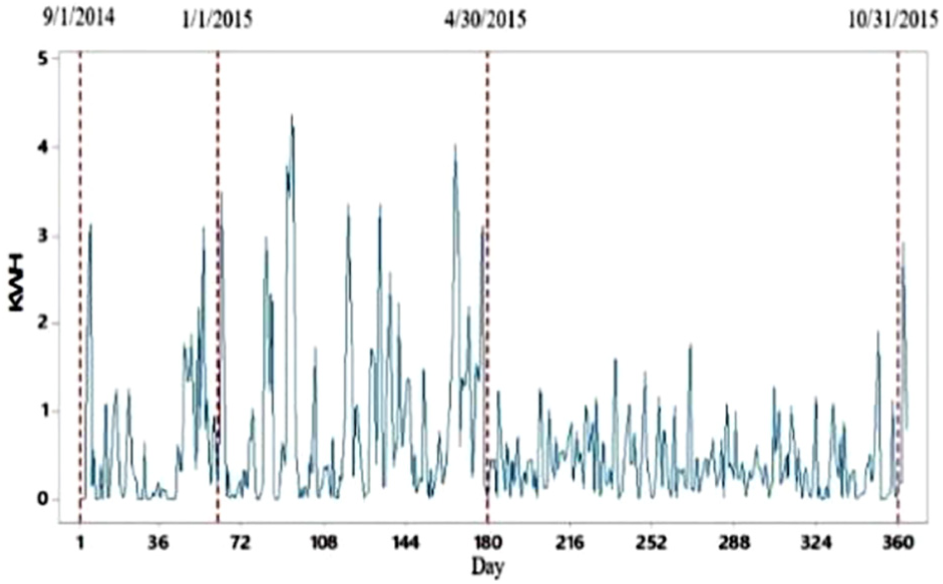
Actual data and relevant dates—beginning and ending of populations within original data.

After these considerations, this dataset was divided into two time series: one from 1 November to 30 April covering the coldest weather months that present higher DOE peaks, starting at the end of the hurricane season and finishing in the middle of spring. The second covers the rest of the dataset, until 31 October. This is why it was proposed to treat this dataset as two series: high-power sample (HPS) and low-power sample (LPS). In Figure 7, the dates of starting and ending of each series, as well as 1 January as a reference, are highlighted.

Seasonality analysis and series decomposition

The analyzed time series is the energy produced by a wind turbine, which is highly dependent on weather-related measurements. Given its origin, the climatological variables can present characteristics of seasonality, so it is advisable to determine whether the series in question has these characteristics.³⁴ This becomes relevant because such seasonality must be included in a seasonal ARIMA model (sARIMA) if it exists.

There are some indicators that help to identify if the effects of seasonality are relevant in time series, such as the autocorrelation and partial autocorrelation functions. For the original data, no obvious patterns appear throughout the series, see Figure 6.

To confirm the first intuition generated by the ACF and the PACF, the graph of the moving averages of the original time series can be obtained, which also facilitates the identification of the patterns. When patterns appear or the probability distribution of the residuals are far from a normal distribution, the time series can be assumed as a seasonal time series.³⁴

Figure 8 shows the original series and the graph of the moving averages every 15 days. In the first part of the series, called HPS, a seasonal pattern appears, while for the rest of the data, the low-power part, no patterns are observed.

Figure 8.

Actual time series starting from 1 November 2014 to 31 October 2015 and moving average.

For more clarity, see Figure 9, which shows only the data in the high-power regime and the corresponding moving averages. A seasonal pattern is identified. In addition, in Figure 10, the autocorrelation function is shown for a 15-data lag and its high relevance is revealed. Each new time series was stabilized in the variance and later the second differentiation was applied to both. In Figure 11, HPS and LPS as well as their histograms are presented. It is clear that both datasets have Weibull distribution, while LPS may have a possible outlier; this analysis was not conducted.

Figure 9.

HPS and moving averages with a length of 15.

Figure 10.

ACF of 15-data lag.

Figure 11.

(a) DOE from 1 November 2014 to 30 April 2015 (HPS). (b) Histogram of HPS. (c) DOE from 1 May 2015 to 31 October 2015 (LPS). (d) Histogram of LPS.

Figure 12 shows both stabilized series using the first differentiation and also the ACF and PACF of the second differentiation for HPS and LPS can be observed. In this way, it can be identified the part of ARIMA model for each case; obviously, for the seasonal time series, a seasonal component will be added.

Figure 12.

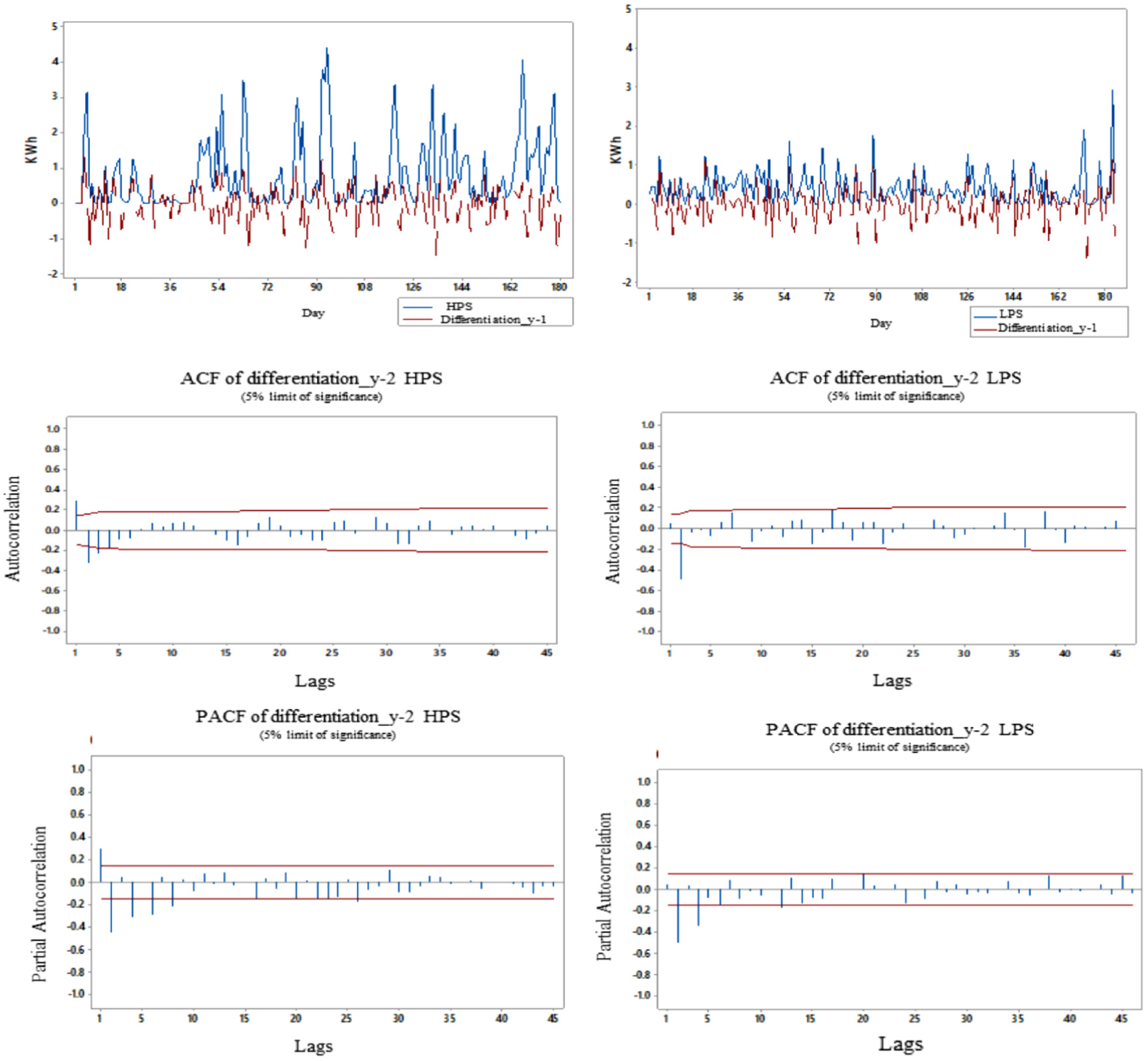
Stabilized series, ACF and PACF. Left: HPS. Right: LPS.

Analyses showed that the first and second lag seemed to be really significant to HPS, while for LPS the first lag did not appear to be highly relevant; nevertheless, second and fourth lag showed some relevance. A performance analysis of predictions of the sARIMA model for HPS and some ARIMA models for LPS forecasts was carried out as well as a comparison against the Pm as seen in section “Methodology.” The Pm is also presented as y_t_– 1. Generally, when making predictions, one-step-ahead to have a good performance of Pm is expected. Table 4 shows the results of prediction models for both regimes, as well as Pm of both HPS and LPS. Computing MAE and MSE measures the prediction accuracy.

Table 4.

Normalized MAE and MSE values of ARIMA models and Pm: HPS and LPS.

HPS				LPS
Model	Equation	MAE	MSE	Model	Equation	MAE	MSE
Pm	$Y_{t} = Y_{t - 1}$	0.157	0.220	Pm	$Y_{t} = Y_{t - 1}$	0.146	0.173
sARIMA (0,1,1) (0,1,1)₁₅	$Y_{t} = Y_{t - 1} + Y_{t - 15} - Y_{t - 16} + e_{t} - 0.3664 e_{t - 1} - 0.8665 e_{t - 15} + 0.3174 e_{t - 16}$	0.155	0.212	ARIMA (1,1,0)	$Y_{t} = - 0.00328 - 0.4879 Y_{t - 1} + Y_{t - 1} - 0.4879 Y_{t - 2} + e_{t}$	0.161	0.176

MAE: mean absolute error; MSE: mean square error; Pm: persistence model; HPS: high-power sample; LPS: low-power sample; ANN: artificial neural network.

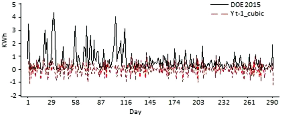
Quantitatively, in Table 4, the sARIMA model presented lower error values than Pm for high power data, while for low regime data, these values were higher. This may be due to the fact of the lower variations of LPS. Hence, hypothesis that there are two populations within these data was confirmed, this also support the decision of treat them separately. Figure 13 presents the sARIMA and ARIMA models from Table 4 as well as the actual curve and the Pm. In the case of sARIMA model for HPS, a slight offset is presented, while in the case of the two ARIMA models for LPS, it seems like they do not achieve a great fitting to actual curve. Persistence has a natural offset in both cases.

Figure 13.

(a) sARIMA model of HPS. (b) ARIMA models of LPS.

The final decision to select the most suitable FM to make a prediction of a time series should accomplish both quantitative and qualitative tests. Therefore, for HPS, the model is sARIMA (0, 1, 1) (0, 1, 1)15 that includes the seasonal pattern every 15 lags, without considering autoregressive properties. While, for LPS, none of the ARIMA models, get lower MAE and MSE values than Pm, in the figure we present two models that best fit the actual curve.

Figure 13 shows the real data, the most common model to predict the wind speed called persistence ( $y_{t - 1}$ ) and the generation of a time series called synthetic series, which is obtained by applying the sARIMA model. To obtain the synthetic series, the observations of the real series are necessary; for our case, we need the observations $y_{t - 1}$ , $y_{t - 15}$ , and $y_{t - 16}$ . With the synthetic series generated, it is possible to compare the performance of the sARIMA model and the Pm through the forecasting error measurements MAE and MSE.

The sARIMA model and the NAR model should perform better than persistence to make them worthwhile. Finally, the sARIMA model will be used in prediction a step forward, where there is no real data, that is, $y_{t}$ of the obtained equation by sARIMA becomes $y_{t + 1}$ ; $y_{t - 1}$ is the last data of the wind speed we know, and $y_{t - 15}$ and $y_{t - 16}$ become $y_{t - 14}$ and $y_{t - 15}$ , respectively. So, the prediction of wind speed is generated one step forward, called forecast outside the sample.

After obtaining these results and due to the fact that ARIMA models failed to outperform persistence when forecasting LPS, a NAR to forecast this time series was produced; to this purpose, MATLAB^® packages were employed.

NAR

Neural networks have a layered structure. This structure is composed by an input layer, some hidden layers and an output layer. Hidden layers usually work as a black boxes where information of the input layer is decomposed through some operations and distributed on their neurons with different “weights”. Afterwards, thanks to other operations, the output layer presents the result of the NAR.

The number of configurations of neural networks to produce forecasts is quite large, depending on the type of variables to be forecasted. The most important characteristics that modify the performance of neural networks and enable them to produce suitable forecasts for each particular case study are their structure and the selection of the internal function to perform the weight distribution.²⁷

Figure 14 shows the default NAR design of MATLAB. The firs module in the figure Y(t) are the observations or the variable. It has a hidden layer that spreads the weight of the inputs by a sinusoidal function that has 15 neurons and 2 lags. Finally, the output layer makes a linear operation to regroup the weights from the neurons in the previous layer and gives a single result or forecast. In our case study, to produce a NAR that had a sufficiently good performance of the validation phase, many tests were carried out by changing, heuristically, the number of neurons and number of lags as well as the percentage of data to be used in the training phase.

Figure 14.

Structure of a NAR with sinusoidal function.³⁵

In Table 5, the results of MAE and MSE of both NAR and Pm are shown. In both cases, the training phase uses 70% of the data, the validation phase uses 15% and 15% (27 points) is reserved to forecast. Due to the size of LPS (187 data), the training phase had trouble to be fully reliable. Nevertheless, two NARs were found and compared to Pm: ANN 187/10-4 and ANN 187/15-2. The code used to name the ANN includes the length of time series, the number of neurons in the hidden layer and the number of lags, that is, ANN 187/15-2 indicates a time series of 187 data, 15 hidden neurons, and 2 lags.

Table 5.

Normalized values for NAR models (using information of LPS (187 observations)).

Model	Equation	MAE	MSE
Pm	$Y_{t} = Y_{t - 1}$	0.146	0.173
ANN 187/10-4	10 neurons in hidden layer and 4 lags	0.144	0.134
ANN 187/15-2	15 neurons in hidden layer and 2 lags	0.164	0.156

NAR: non-autoregressive; LPS: low-power sample; Pm: persistence model; MAE: mean absolute error; MSE: mean square error; ANN: artificial neural network.

Due to the difficulties that training phase presented, to rely only on this information may mislead one to an erroneous conclusion, thus it is mandatory to contrast the prediction to real series and Pm plot.

In Table 6, the results of MAE and MSE of Pm and two NAR are shown: ANN 365/4-2 and ANN 365/10-2. In these cases, an 80% of data was utilized in the training phase, 10% in the validation phase, and 10% to forecast. In both cases, training difficulties where reduced. Also, more reliable models than in the case where only LPS data were used, were produced. Additionally, both ANN achieved had lower error measurements than Pm.

Table 6.

Normalized values for NAR models (using information of whole series (356 observations)).

Model	Equation	MAE	MSE
Pm	$Y_{t} = Y_{t - 1}$	0.145	0.112
ANN 365/4-2	4 neurons in hidden layer and 2 lags	0.092	0.107
ANN 365/10-2	10 neurons in hidden layer and 2 lags	0.060	0.079

NAR: non-autoregressive; Pm: persistence model; MAE: mean absolute error; MSE: mean square error; ANN: artificial neural network.

In Figure 15, the predictions of ANN 187/15-2 and ANN 187/10-4 for the LPS are shown. Even though both ANN had a lower value for MAE and MSE, they do not fit the path of the real series, especially in those observations equal to zero.

Figure 15.

NAR forecasts, persistence, and actual curve of LPS (187 observations).

In Figure 16 the resulting prediction of ANN 365/10-2 and ANN 365/4-2 for the low powered regime is shown along with the actual data and the Pm. In both cases, a closer following of actual data is evident. As observed in the case of the sARIMA model, the actual data are used to compare and to obtain error measurements, and a forecast outside the sample is presented. ANN 365/10-2 has a behavior very similar to Pm; nevertheless, the model beats Pm in the error measurements. Evidently, having more data and defining a larger training phase resulted in a better fitting to actual curve, considering that in this case an 80-10-10 percentage share was applied as recommended in the literature.

Figure 16.

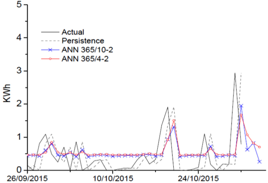
NAR forecasts, persistence, and actual curve of LPS (365 observations).

In Table 7, the improvement regarding to Pm of the corresponding models is shown.

Table 7.

Improvement of models compared to Pm.

Model	% improvement of MAE	% improvement of MSE
sARIMA (0,1,1) (0,1,1)₁₅	0.2%	0.8%
ANN 187/10-4	0.2%	3.9%
ANN 365/10-2	8.5%	3.3%

Pm: persistence model; MAE: mean absolute error; MSE: mean square error; ANN: artificial neural network; sARIMA: seasonal ARIMA.

Selection of FM

In time series such as the one in the described problem, there are periods in which it is not possible to define in a simple way if the series will behave as a series of low or high power. In fact, there are occasions when there is an overlap of both behaviors. Therefore, it can be complicated to select the ad hoc model to predict DOE in the current time. This indicates the need to have a method for the standardized selection of the FM to be used.

Furthermore, since in the presented case study each point in the time series represents the daily cumulative value of the wind turbine power production, each value of the forecast, even if it is a step forward, includes the following 24 h; therefore, it is affected by atmospheric dynamics. As can be seen in Giebel et al.,³⁶ Monteiro et al.³⁷ for wind energy forecasts beyond 6 h ahead, it is known that purely statistical prediction models do not have performances as good as NWP models, since the latter represent better atmospheric changes.^36–39

As can be seen, given the conditions of the current problem, it is necessary to involve an analysis that will help (1) to discern in an objective (standardized) manner if the time series will be in the high or low power regime and (2) to increase the effectiveness of the NAR or sARIMA models when they are implemented.

In order to identify the type of time series that is currently in place, we must consider what has happened in the recent past, as well as identify a trend in the future. To visualize the past, the average of the DOE of the previous 15 days is recorded to have an initial estimation.

For the visualization of the future, it has been considered to use a known NWP in the scientific environment, the WRF model, in order to predict the wind behavior for the study site for the following 24 h in 6-h intervals. This will help to estimate what the wind speed process will be like, which will allow, in combination with the DOE average, to select the ad hoc DOE FM. The following section describes the characteristics of the WRF model, its application for the study site, as well as its role in the selection a FM of DOE.

Parameters of WRF for the study site

The numerical simulations were performed with the WRF model in its version 2.84 for a parent domain, D1, with a spatial resolution of 45 km, and two nested domains, D2 and D3, with spatial resolution of 15 and 5 km, respectively, as observed in Figure 17. The mother domain is centered at 19:768° N and 101:189° W, with a LAMBERT map projection and 27 eta levels in the vertical.

Figure 17.

Domains of WRF model. D1 with 45 km resolution; D2 with 15 km resolution; D3 with 5 km resolution.

The physical parametrizations used for this study are shown in Table 8.

Table 8.

WRF main technical characteristics.

Physical parametrizations	Schemes
Planetary boundary layer	Mellor–Yamada–Nakanashi–Niino levelTKE (MYNN)
Microphysics	WRF simple-moment 3-class (WSM3)
Longwave radiative	Rapid radiative transfer model (RRTM)
Short-wave radiative	Dudhia
Cumulus	Kain–Fritsch
Surface layer	Monin–Obukhov similarity theory

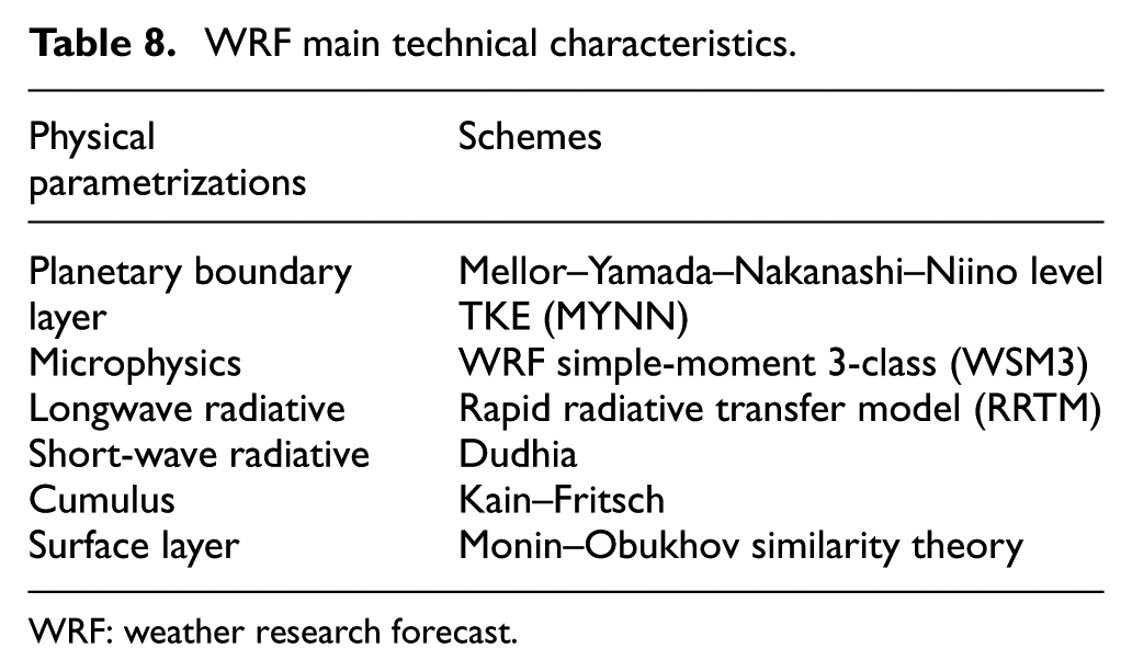
WRF: weather research forecast.

An analysis of the wind speed is made and a forecast of the following day is delivered in 6-h intervals. This is done to see a trend or future behavior of the wind speed, as shown in Figure 18. This information will be analyzed to discern if, at the current time, the data is in a low-power or high-power regime, as will be discussed below.

Figure 18.

Wind speed prediction for the next day with 6-h averaged forecast.

Identifying LPS and HPS

To have greater certainty about the power regime that occurs in the current time, be it HPS or LPS, first the average of the previous days of the DOE is calculated as a reference. In the event that the average has a value higher than the LPS average, this may indicate that the time series is an HPS.

In the case in which the average speed estimated by the WRF is close to the nominal speed of the turbine, in addition to a high DOE average of the previous 15 days, it can be concluded that the current measurement corresponds to the high-power regime. Only in the case in which both of the verification processes are true, the current data will be considered as a high-power time series; in any other case, it will be considered as a low power time series. In the flow chart in Figure 19, the process of identification between LPS and HPS is shown.

Figure 19.

Flow chart of the identification process to define high or low regime process.

The wind dependable time series, being meteorological data, generally have variable velocity values. Average speeds may vary on a monthly, seasonal, or annual basis.

To generate a prediction model with statistical techniques such as sARIMA, or with artificial intelligence techniques such as NAR, it is necessary to have historical data and analyze the general behavior of them. It is possible, therefore, to identify patterns where the wind speeds are high or of lower intensity. In these periods of time, we can propose the model that presents the best prediction results (sARIMA, NAR, in our case). On the other hand, the WRF model can be used anywhere in the world; therefore, the proposed method can be applied as a general method to forecast the wind speed. However, the final decision must be made by the forecaster after analyzing his historical.

Conclusion

In this article, the forecast of wind power is presented by identifying a sARIMA and NAR models to predict one step ahead of DOE of a XZERES Skystream 3.7 wind turbine, placed in Morelia, Mexico. Initial results of ARIMA models applied to a yearly dataset of DOE performed poorly. A deeper analysis of actual data showed evidence of a double behavior along a year. Thus, by an inspection and visual correlation, it was proposed to separate original time series into two populations: HPS and LPS, one with greater power range than the other.

It was decided to treat HPS and LPS separately. The high-power regime was located between November of 2014 and the end of April of 2015. The low powered data comprehends from May to October of 2015, completing 12 consecutive months, hence a year of historic data. A review of the seasonality present in the data was made, finding that the data of the high-power regime have a seasonal pattern every 15 steps, while the low power one does not have an evident seasonal pattern.

In the HPS, a sARIMA model that had lower error measurements than the Pm is propose, while for the LPS none of the ARIMA models had a better performance than Pm. Hence, it was proposed to use NAR models to predict LPS.

Afterwards, two NAR models to predict low power regime were determined. On a first approach, NAR models used just LPS data (187), which provoked poor training performances, hence low reliability. Nevertheless, their error measurement is lower than the one of Pm, although they do not properly fit actual curve. Due to the contradictory results, a new approach was considered: to utilize the whole dataset to obtain better training performance.

Utilizing 365 data in a 80-10-10 percentage share, allowed to produce two NAR models with reliable training performances and better error measurements than in the first approach. And even more, they fitted better to actual curve than the NAR models that only utilized 177 data.

It is possible that the difficulties to obtain FMs (particularly, ARIMA models) to forecast LPS with better performance than Pm may be related to the lower variations of this regime and the reduced number of observations available. However, it was demonstrated that even with small samples, the propose sARIMA model can produce better results of error measurements than Pm, for example, in HPS where “high” variations of data provoke higher error measurements of the Pm. At the same time, small samples resulted in training issues of NAR models hence unreliable models, for example, the case of using only LPS data resulted in a lower error measurement of Pm but a poor fitting of actual curve. However, NAR models that use more data to complete training phase had reliable training performances, the lowest error measurements and a better fitting to actual curve of low power regime dataset.

To select which of the proposed models to use, we must know if a regime with seasonality and high power is happening or, on the contrary, the current time corresponds to the case of non-seasonality and low power regime. For this, the DOE average of the previous 15 days and the forecast of the wind speed of the future 24 h obtained by means of a numerical weather prediction model (WRF), are necessary. With this information, the forecaster can know in advance the ad hoc model to forecast the DOE for the next day.

The presented sARIMA and NAR models demonstrated that had strengths and weaknesses; however, forecasters can take this into consideration and try to exploit, without bias, both approaches. It is not simply about which approach (ARIMA or NAR) is better, it is about the specific goals and scope of each case study, and how they can be cover using all information available and all techniques in the literature.

Footnotes

Acknowledgements

The authors would like to recognize the excellent facilities and all dispositions showed during the data acquisition by the Electric Engineering Faculty staff.

Handling Editor: Gang Xiao

Declaration of conflicting interests

The author(s) declared no potential conflicts of interest with respect to the research, authorship, and/or publication of this article.

Funding

The author(s) received no financial support for the research, authorship, and/or publication of this article.

ORCID iD

Jorge Luis Tena García

References

Garcia-Heller

Espinasa

Paredes

Forecast study of the supply curve of solar and wind technologies in Argentina, Brazil, Chile and Mexico. Renew Energ 2016; 93: 168–179.

Deshmukh

Modeling of hybrid renewable energy systems. Renew Sust Energ Rev 2008; 12: 235–249.

Cadenas

Rivera

Wind speed forecasting in three different regions of Mexico, using a hybrid ARIMA–ANN model. Renew Energ 2010; 35: 2732–2738.

Vaara

Pitkänen

Hämäläinen

Wind turbine sensor data analysis and production forecast. In: European modelling symposium (EMS), Pisa, 21–23 October 2014, pp.309–314. New York: IEEE.

Murugan

Umamaheswari

Vimal

et al . Experimental investigation on power output in aged wind turbines. Adv Mech Eng 2012; 4: 380986.

Stathopoulos

Kaperoni

Galanis

et al . Wind power prediction based on numerical and statistical models. J Wind Eng Ind Aerodyn 2013; 112: 25–38.

Goretti

Duffy

Lie

. The impact of power curve estimation on commercial wind power forecasts—an empirical analysis. In: Proceedings of the 14th international conference on the European energy market (EEM), Dresden, 6–9 June 2017, p.14. New York: IEEE.

Nagaraja

Devaraju

Kumar

et al . A survey on wind energy, load and price forecasting: (Forecasting methods). In: International conference on electrical, electronics, and optimization techniques (ICEEOT), Chennai, India, 3–5 March 2016, pp.783–788. New York: IEEE.

Nguyen

Metzger

Comparison of forecasting methods for vertical axis wind turbine applications in an urban/suburban area. J Renew Sust Energ 2017; 9: 023302.

10.

Cadenas

Rivera

Campos-Amezcua

et al . Wind speed forecasting using the NARX model, case: La Mata, Oaxaca, Mexico. Neural Comput Appl 2016; 27: 2417–2428.

11.

Park

Son

Park

et al . An irradiation prediction model for photovoltaic power generations under limited weather information. IFAC Proc Vol 2014; 47: 3670–3675.

12.

Martin

Zhang

Chan

et al . A comparison of Gumbel and Weibull statistical models to estimate wind speed for wind power generation. In: Australasian universities power engineering conference (AUPEC), Perth, WA, Australia, 28 September–1 October 2014, pp.1–6. New York: IEEE.

13.

Masrur

Nimol

Faisal

et al . Short term wind speed forecasting using artificial neural network: a case study. In: International conference on innovations in science, engineering and technology (ICISET), Dhaka, Bangladesh, 28–29 October 2016, pp.1–5. New York: IEEE.

14.

Castellani

Astolfi

Mana

et al . Wind power forecasting techniques in complex terrain: ANN vs. ANN-CFD hybrid approach. J Phys Conf Ser 2016; 753: 082002.

15.

Veit

Goebel

Tidke

et al . Household electricity demand forecasting: benchmarking state-of-the-art methods. In: Proceedings of the 5th international conference on future energy systems, Cambridge, 11–13 June 2014, pp.233–234. New York: ACM Press.

16.

D’Amico

Petroni

Prattico

Wind speed and energy forecasting at different time scales: a nonparametric approach. Physica A 2014; 406: 59–66.

17.

Croonenbroeck

Dahl

CM.

Accurate medium-term wind power forecasting in a censored classification framework. Energy 2014; 73: 221–232.

18.

Kay

The application of TAPM for site specific wind energy forecasting. Atmosphere 2016; 7: 23.

19.

Staid

Pinson

Guikema

SD.

Probabilistic maximum-value wind prediction for offshore environments. Wind Energ 2015; 18: 1725–1738.

20.

Wilczak

Finley

Freedman

et al . The wind forecast improvement project (WFIP): a public–private partnership addressing wind energy forecast needs. B Am Meteorol Soc 2015; 96: 1699–1718.

21.

Han

Romero

Yao

Wind power forecasting based on principle component phase space reconstruction. Renew Energ 2015; 81: 737–744.

22.

Ulkat

Günay

. Prediction of mean monthly wind speed and optimization of wind power by artificial neural networks using geographical and atmospheric variables: case of Aegean Region of Turkey. Neural Computing and Applications 2018; 30: 3037–3048.

23.

Koçak

Practical ways of evaluating wind speed persistence. Energy 2008; 33: 65–70.

24.

Hayashi

Nagasaka

. Wind speed prediction and determination of wind power output with multi-area weather data by deterministic chaos. In: Proceedings of the international conference on advanced mechatronic systems (ICAMechS), Kumamoto, Japan, 10–12 August 2014, pp.192–197. New York: IEEE.

25.

Yuan

Tan

Lei

et al . Wind power prediction using hybrid autoregressive fractionally integrated moving average and least square support vector machine. Energy 2017; 129: 122–137.

26.

Sharma

Ghosh

Short-term wind speed forecasting: application of linear and non-linear time series models. Int J Green Energ 2016; 13: 1490–1500.

27.

Cadenas

Rivera

Wind speed forecasting in the south coast of Oaxaca, Mexico. Renew Energ 2007; 32: 2116–2128.

28.

Xiao

Wang

Dong

et al . Combined forecasting models for wind energy forecasting: a case study in china. Renew Sust Energ Rev 2015; 44: 271–288.

29.

Nielsen

MA.

Neural network and deep learning. Determination Press, 2015, http://neuralnetworksanddeeplearning.com/

30.

Siuta

West

Stull

WRF hub-height wind forecast sensitivity to PBL scheme, grid length, and initial condition choice in complex terrain. Weather Forecast 2017; 32: 493–509.

31.

Eleftheriadou

Sfetsos

Gounaris

The suitability of high resolution downscaled seasonal models for the energy assessment of the building sector. Energ Buildings 2016; 111: 176–183.

32.

Plante

Dyck

et al . An operational application of NWP models in a wind power forecasting demonstration experiment. Wind Engineering 2014; 38: 1–21.

33.

Xzeres. Wind Turbine products. Xzeres Skystream 3.7 product information. Xzeres, http://www.xzeres.com/wind-turbine-products/xzeres-skystream-3-7wind-turbine/ (2012, accessed January 2017).

34.

Makridakis

Wheelwright

Hyndman

RJ.

Forecasting: methods and applications. Hoboken, NJ: John Wiley & Sons, 2008.

35.

Demuth

Beale

Hagan

Neural network toolbox TM 6: user’s guide, vol. 10. Natick, MA: MathWorks, 2008.

36.

Giebel

Brownsword

Kariniotakis

et al . The state-of-the-art in short-term prediction of wind power: a literature overview. ANEMOS Plus, 2011.

37.

Monteiro

Bessa

Miranda

et al . Wind power forecasting: state-of-the-art 2009. Technical report, Argonne National Lab (ANL), Lemont, IL, 6 November 2009.

38.

Foley

Leahy

Marvuglia

et al . Current methods and advances in forecasting of wind power generation. Renew Energ 2012; 37: 1–8.

39.

Costa

Crespo

Navarro

et al . A review on the young history of the wind power short-term prediction. Renew Sust Energ Rev 2008; 12: 1725–1744.

Forecast of daily output energy of wind turbine using sARIMA and nonlinear autoregressive models

Abstract

Keywords

Introduction

Forecast models

Forecast horizons

Persistence

ARIMA models

ANN

NWP models

Hybrid models

Forecast validation

Methodology

Case of study

Results

ARIMA and sARIMA models

Seasonality analysis and series decomposition

NAR

Selection of FM

Parameters of WRF for the study site

Identifying LPS and HPS

Conclusion

Footnotes

Acknowledgements

Declaration of conflicting interests

Funding

ORCID iD

References