Sage Journals: Discover world-class research

Abstract

Background

A substantial increase in the incidence of immediate release fentanyl (IRF) use was reported in Spain from 2012 to 2017.

Purpose

This study aimed to investigate the relationship dynamically with cancer incidence in order to provide empirical evidence of inappropriate use of IRF with respect to the pathology.

Research design

A vector autoregresive (VAR) model was constructed using data from a nationwide electronic healthcare record database in primary care in Spain (BIFAP) according to the following step procedure: (1) split data into training data for modelling and test for validation (2) assessing for time series stationarity; (3) selecting lag-length; (4) building the VAR model; (5) assessing residual autocorrelation; (6) checking stability of the VAR system; (7) evaluating Granger causality; (8) impulse response analysis and forecast error variance decomposition (9) prediction performance with validation data.

Results

The analysis showed a strong and linear correlation between IRF and cancer (Pearson correlation coefficient: 0.594 (95% CI: 0.420–0.726). Two VAR models, VAR (2) and VAR (11) were selected and compared. All tests performed for both models satisfied assumptions for stability, predictability and accuracy. Granger causality revealed cancer incidence is a good predictor for IRF use. VAR (2) seemed to be slightly more accurate, according to the RMSE of the test data.

Conclusions

This study demonstrates that using a robust and structured VAR modelling approach, is able to estimate dynamics associations, involving IRF use and cancer incidence.

Keywords

Fentanyl time series analysis forecasting cancer pain pharmacoepidemiology pharmacovigilance

Introduction

Over the past decade, opioids use has increased in the European Union (EU), being fentanyl the most frequently consumed opioid analgesic in many countries.^1–3 A 53% increase in the incidence of immediate release fentanyl (IRF) use was reported in Spain from 2012 to 2017.⁴ Despite this increase, we are not aware of studies investigating the extent of its relationship with trends in cancer incidence. In the EU, IRF is only approved for use in patients with breakthrough cancer pain (BTCP) who are already receiving opioids maintenance therapy (OMT) for chronic cancer pain, unlike other short acting opioids, such as morphine, oxycodone or hydromorphone, also considered appropriate for some transient pain types in non-cancer patients.⁵ Benefit of IRF outweighing the risk of dependence and abuse has not been demonstrated in this population.^6–12 Assessing the trend in cancer incidence and its dynamic relationship with IRF use, might provide an approximation on the extent of IRF inappropriate use.

Multivariate time series analysis using vector autoregressive (VAR) models, is one of the most flexible and comprehensible method to explain past and causal relationships among multiple variables over time, as well as predict future observations.^13,14 VAR technique has also the ability to separate the dynamic longitudinal part, from the simultaneous part of the associations between variables, and correcting for potential feedback effects. A VAR model consists of a set of regression equations, in which each of the variables is regressed on its own lagged values (autocorrelation) as well as the lagged values of the other variables (cross-lagged associations).^13–15 The novelty of this research in the field of pharmacovigilance lies in the fact that VAR models might be useful to detect relationships between the use of drugs and the disease for which they are indicated, considering the lags between the date of diagnosis and the date of drug prescription, obtaining hypotheses that might explain the usage trends.

Therefore, modeling IRF use and its dynamic associations with cancer incidence, could allow us to contextualize the increase in IRF use observed in Spain last decade and future assessments on the effectiveness of risk minimization measures put in place by regulatory authorities in order to contain its use.

Methods

Design and source of data

Ecological study between 1st January 2012 to 31st December 2017 conducted in BIFAP, an electronic healthcare record (EHR) database from primary care in Spain, already validated through previous multiple studies^4,16 and successfully compared with other well-known European databases.^16,17 Over the study period, BIFAP included anonymized information from nine million of patients covering almost 20% of the Spanish population, with an average follow up of 7.2 years, from nine regions providing data. Clinical events are recorded by using the International Classification of Primary Care (ICPC-2) and the International Classification of Disease (ICD-9).^18,19

Variables definition

Exposure to IRF was defined with the ATC code N02AB03²⁰ and the national product code of all immediate release forms marketed in Spain, in order to exclude fentanyl transdermal patches (for more information on the pharmaceutical formulations included in the study see Table S1).

Potential cancer cases on malignant neoplasm were identified using ICPC-2 and ICD-9 codes. Non-melanoma skin cancer codes were excluded (see complete list of ICPC-2 and ICD-9 codes in Table S2).

Study population

For the IRF exposed time series, new users of IRF were identified by excluding patients with a prescription of IRF, any time before the date of the first prescription in the study period.

For the cancer exposed time series, new cancer patients diagnosed were identified by excluding patients with a diagnosis of cancer, any time before the date of the first diagnosis in the study period

Statistical analysis

Monthly cumulative incidences per 100,000 patients for IRF and cancer, were calculated by dividing the number of new IRF users or new cancer diagnosed patients respectively, by the number of patients from the study population (with at least 1 day of follow up) in the corresponding period of calculation (month).

A vector autoregressive (VAR) model was developed to investigate the dynamic associations between changes in the incidence of cancer and incidence of IRF use, using the following step procedure:

Data preprocessing

First, the available data was split into training data, from 1st January 2012 to 31st December 2016, and test data, from 1st January 2017 to 31st December 2017. The training data were used to estimate the parameters of the forecasting method and the test data were used to evaluate its accuracy. Because the test data was not used in determining the forecast, it should provide a reliable indication of how well the model is likely to forecast on new data. The size of the test set is typically about 20% of the total sample, although this value depends on how long the sample is and how far ahead we want to forecast.

Testing stationarity

Stationary time series are detrended series, without periodic fluctuations. Stationarity is critical for developing of a VAR model because in its absence, a model´s statistics such as means and correlations will not accurately describe the time series signal. Stationarity of the time series was checked using the augmented Dickey-Fuller test. The null hypothesis is that the time series is non-stationary and it rejection indicates that the series does not need transformation to achieve stationarity.¹⁴ Differencing or data log transformation were performed, in order to stabilize the variance and mean, respectively, if the stationarity assumption of the time series was violated.

Selecting lag length

Lag length selection refers to the number of previous observations in a time series that will be used as predictors in the VAR model. For example, a p^th order VAR, refers to a VAR model which includes values of the variables for the last p months. The most common approach to select the lag is to fit VAR (p) models with orders p = 0, 1. p_max, and choose the VAR model with the minimum value of the Akaike Information Criterion (AIC), Bayesian Information Criterion (BIC) and Hannan-Quinn (HQ) criterion.^13,21

Building the vector autoregressive model

The parameters of the VAR model were estimated using the method Ordinary Least Squares (OLS). It involves minimizing the sum of squared residuals between the observed values and the values predicted by the model to obtain the coefficient estimates.

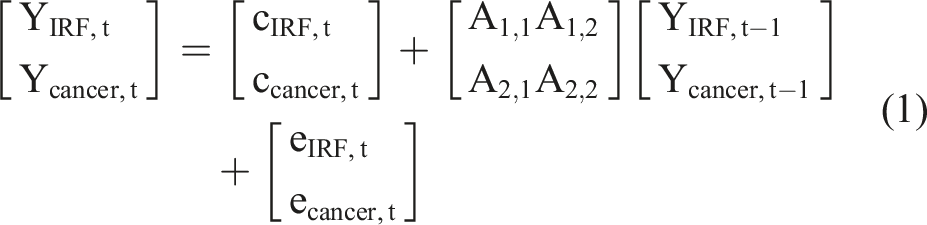
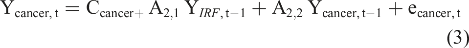
The general structure of the VAR model is that each variable, at a point in time, is a linear function of the most recent lag of both itself and the other variables. The equations of a VAR(1) model for two time series, for example IRF and cancer, has the usual matrix form for a regression equation with multivariate outcomes, such that:

[\begin{array}{l} Y_{IRF, t} \\ Y_{cancer, t} \end{array}] = [\begin{array}{l} c_{IRF, t} \\ c_{cancer, t} \end{array}] + [\begin{array}{l} A_{1,1} A_{1,2} \\ A_{2,1} A_{2,2} \end{array}] [\begin{array}{l} Y_{IRF, t - 1} \\ Y_{cancer, t - 1} \end{array}] + [\begin{array}{l} e_{IRF, t} \\ e_{cancer, t} \end{array}]

(1)

or, in scalar notation:

Y_{IRF, t} = C_{IRF +} A_{1,1} Y_{IRF, t - 1} + A_{1,2} Y_{cancer, t - 1} + e_{IRF, t}

(2)

Y_{cancer, t} = C_{cancer +} A_{2,1} Y_{I R F, t - 1} + A_{2,2} Y_{cancer, t - 1} + e_{cancer, t}

(3)

The regressors (predictors) of each outcome are the same, which correspond to the lagged values of IRF and cancer. Intercepts terms are indicated by C. A indicates the regressions coefficients and e indicates error in prediction of each outcome at time t.^13,14,22

The error terms should satisfy the following conditions:

1. Zero mean: The errors in a VAR model must equal zero, which means that the average value of the errors must be close to zero. This implies that, on average, the model is unbiased in the way it predicts the observed values.

2. Homoscedasticity: The errors must have a constant variance over time. That is, the error term does not vary much as the value of the predictor variable changes.

3. No autocorrelation: The errors in a VAR model must not show serial autocorrelation, which means that there must not be a systematic relationship between the errors in different periods of time. Autocorrelation may indicate that the model has not fully captured the temporal dependency structure in the data.

4. No cross-correlation: The errors between different VAR model equations must not be correlated with each other. This implies that the errors in one variable should not depend on the errors in the other variables in the model. The lack of cross-correlation ensures that each VAR model equation is independent and can provide unique information.

Testing for residual autocorrelation

Portmanteau test was used to check autocorrelation of the residual values (differences between the actual observation and model fitted values) and determine the goodness of fit of the model. No residual autocorrelation is the null hypothesis and the existence of residual autocorrelation is the alternative hypothesis (there is information that has not been accounted for the model).^13,14

Assessing stability of the vector autoregressive model

Stability of a VAR system refers whether the model is a good representation of how the time series evolved over the sampling window period. Stability was evaluated using the roots of the characteristic polynomial of the coefficient matrix A, as in the example in equation (1). A VAR (p) process is stable if all eigenvalues of the companion matrix A have modulus less than 1.²²

Assessing granger causality

Granger causality is one type of relationship between time series. This relationship should not be over-interpreted as truly causal. Granger causality states if the prediction of one time series called x is improved by incorporating the knowledge of a second time series called y. The null hypothesis is defined as no explanatory power is added by jointly considering the lagged values of y and x.²³

Impulse response analysis and forecast error variance decomposition

The impulse response function analyses the response of one variable to a sudden but temporary change in another variable. Additionally forecast error variance decomposition (FEVD) analyses the proportion of the forecast variance of each variable that is attributed to the effects of the other variable.^13,24

Estimating forecast performance measures

The IRF incidences previously held to test the forecasting accuracy, were compared with the actual data observed. The root mean squared error (RMSE) was the measure used, representing the quadratic mean of the differences between predicted and observed values. RMSE is a measure of accuracy that compares forecasting errors of different models for a particular dataset; a value of 0 (almost never achieved in practice) would indicate a perfect fit to the data.²⁵ Also the 95% prediction intervals were estimated in order to provide an estimation of how far ahead the model predicted.²⁶ Prediction intervals increase in length as the forecast horizon increases.

Information on time series analysis and forecasting covering applications of VAR models in detail and tutorials on how to implement VAR models in R with examples and codes for estimating, testing, and forecasting are provided in the references section.^27–30

Results

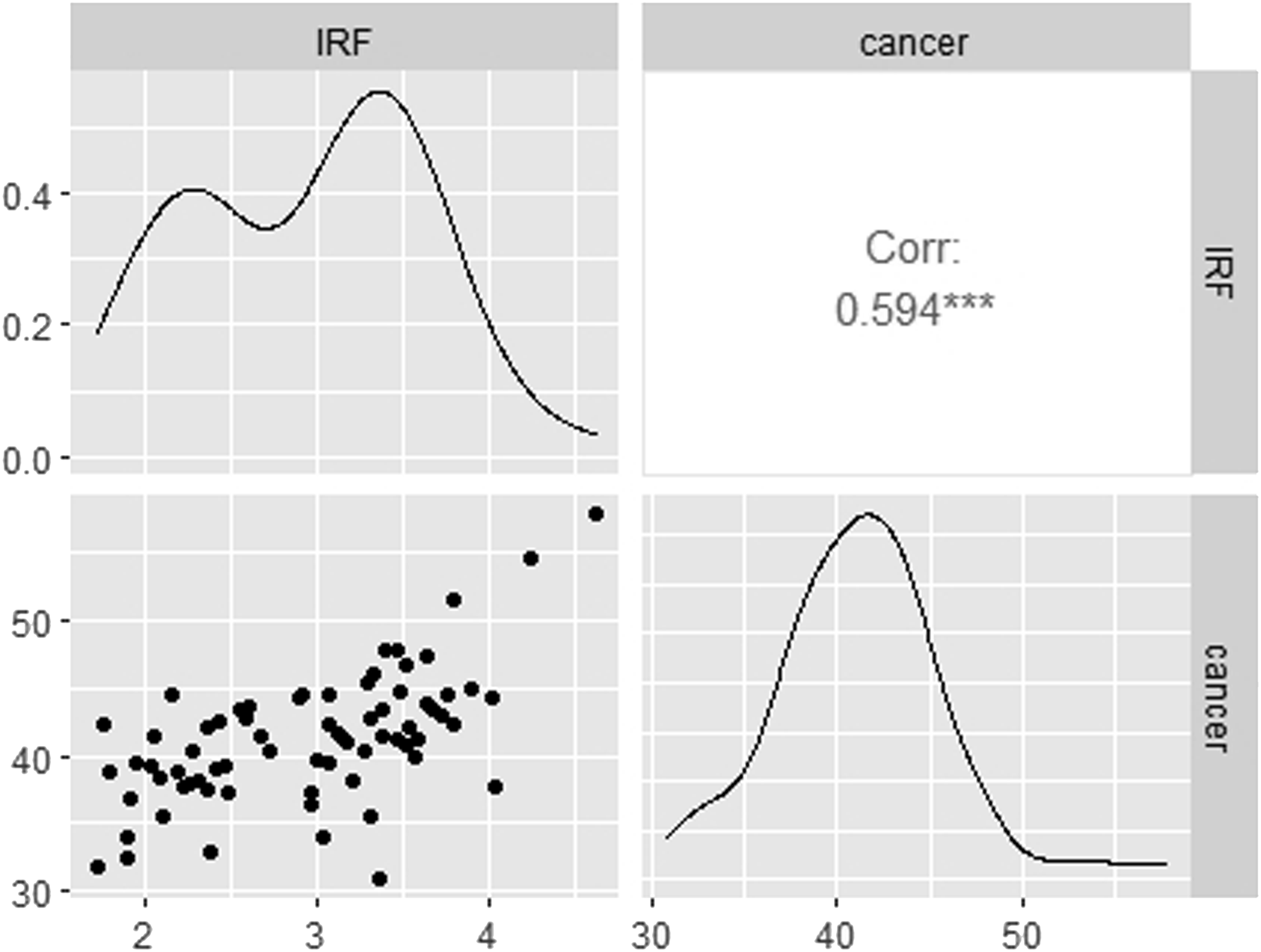
Figure 1 charts data for each variable. From a visual perspective, an upward trend is observed for both time series, cancer and IRF. Figure 2 shows a strong linear correlation between IRF and cancer. Pearson’s correlation coefficient between monthly incidence of cancer and monthly incidence of IRF use was 0.594 (95% confidence interval: 0.420–0.726)

Figure 1.

Illustration of time series plot for monthly incidence of cancer (new cases diagnosed per 100,000 patients) and monthly incidence of immediate release fentanyl (IRF) (new users per 100,000 patients) from 2012 to 2017.

Figure 2.

Scatterplot matrix of the monthly incidence of cancer (new cases diagnosed per 100,000 patients) and monthly incidence of immediate release fentanyl (IRF) (new users per 100,000 patients) from 2012 to 2017. ***p value <.05. For each panel, the variable on the vertical axis is given by the variable name in that row, and the variable on the horizontal axis is given by the variable name in that column. The correlation is shown in the upper right half on the plot, while the scatterplot is shown in the lower half. On the diagonal is shown density plots. The second column shows there is a strong positive relationship between the two variables. Outliers can also be seen. Density plots present the distributions of the variables on a time period, the density in the y axis and the value of the variable in the x axis. The peaks of the density plot display where values are concentrated.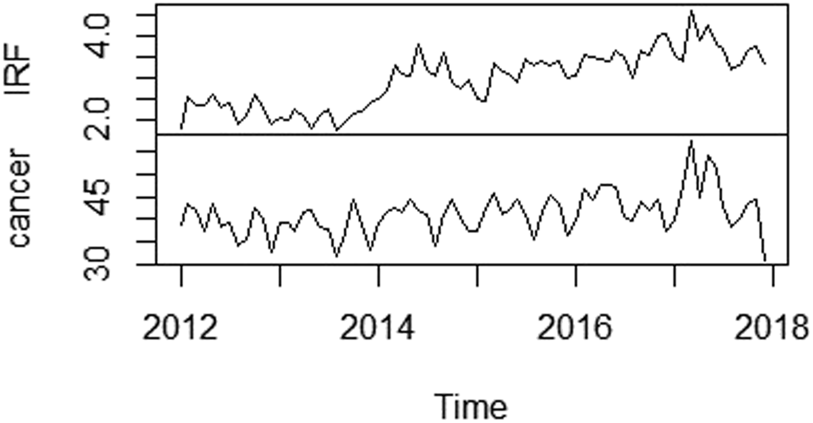

The results of the different tests performed are provided below. Results were significant at p < .05.

The test for stationarity was performed individually for each variable and resulted non-significant (p > .05) for IRF, which indicated that the time series was not stationary. The Dickey Fuller test achieved stationarity after applying first order differencing. Once stationarity was determined, the lag-length selection was estimated. The model with the minimum AIC and HQ was VAR (2), while the minimum value of BIC was for VAR (11). Both models, VAR (2) and VAR (11) were estimated and compared, coefficients are presented in Table 1.

Table 1.

Coefficients of the VAR (2) and VAR (11) models, including the endogenous variables: incidence of immediate release fentanyl (IRF) use per 100,000 patients and incidence of new cancer cases per 100,000 patients.

Regression variable	VAR (2)
	Coefficients for immediate release IRF equation		Coefficients for cancer equation
	Coefficient	p	Coefficient	p
IRF lag1	−0.5001	.0004	−2.2578	.0180
Cancer lag1	0.094	.0365	−0.2215	.0928
IRF lag2	−0.4836	.0005	−1.8536	.2643
Cancer lag2	0.0198	.0610	−0.4427	.0012

Regression variable	VAR (11)
	Coefficients for immediate release IRF equation		Coefficients for cancer equation
	Coefficient	p	Coefficient	p
IRF lag1	−0.2379	.2609	−0.3209	.8196
Cancer lag1	−0.0040	.8550	−0.8233	<.0001
IRF lag2	0.0467	.8478	3.1310	.0648
Cancer lag2	−0.0046	.8265	−0.7610	<.0001
IRF lag3	0.3701	.1449	4.2689	.0160
Cancer lag3	−0.0406	.1366	−0.8345	<.0001
IRF lag4	0.3757	.1373	1.5199	.3651
Cancer lag4	−0.0499	.0994	−0.7233	.0010
IRF lag5	−0.0704	.7829	−2.0591	.2372
Cancer lag5	0.0021	.9410	−0.5778	.0071
IRF lag6	0.0237	.9265	1.0354	.5517
Cancer lag6	−0.0367	.2499	−0.6450	.0049
IRF lag7	−0.1407	.5710	2.7744	.1046
Cancer lag7	−0.0251	.3940	−0.7522	.0006
IRF lag8	−0.3474	.1590	2.1355	.1969
Cancer lag8	−0.0034	.9084	−0.9250	<.0001
IRF lag9	0.0354	.8821	3.5895	.0327
Cancer lag9	−0.0303	.2460	−0.8382	<.0001
IRF lag10	0.1042	.6569	1.6824	.2910
Cancer lag10	−0.0074	.7261	−0.9290	<.0001
IRF lag11	0.0932	.6573	2.3988	.0981
Cancer lag11	−0.0084	.7178	−0.7661	<.0001

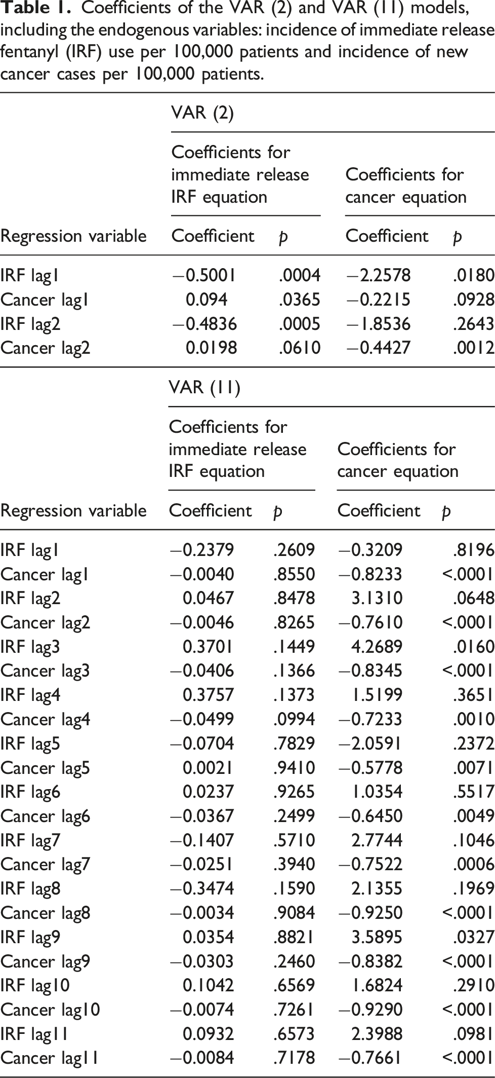
The Portmanteau test indicated no residual serial autocorrelation for VAR (2) (p = .1062) and VAR (11) (p = .0075).

The roots of the characteristics polynomial showed stability for the two VAR models selected. The eigen values of the companion matrix A was computed and their moduli resulted less than 1. Bidirectional causality was also demonstrated after applying the Granger causality test (p < .05).

Figure 3(a)–(d), show the impulse response functions, which are interpreted as how a sudden and temporary change in x, causes significant increases or decreases in y for m periods, determined by the length of period for which the standard error (SE) bands are above or below 0. The bands next to 0 indicate the effect is dissipated. Such interpretation fits well into objectives like how cancer affects IRF and vice versa, when the maximum impact is experienced and for how long the effects last. For the VAR (2) model, the maximum impact for fentanyl response is observed between months 4th and 6th and after the 9th month is dissipated (Figure 3(a)). The maximum impact for cancer response is observed between months 1st and 4th and after the 6th month is dissipated (Figure 3(b)). For the VAR (11), the shock spreads throughout and beyond the 12th month.

Figure 3.

Impulse response functions. (a) Fentanyl response to changes in cancer. Results from the VAR (2) model. (b) Cancer response to changes in fentanyl. Results from the VAR (2) model. (c) Fentanyl response to changes in cancer. Results from the VAR (11) model. (d) Cancer response to changes in fentanyl. Results from the VAR (11) model. The horizontal axis is the plot of the impulse response. The measurement is stated in standard errors (SE). It is not unitized because it is a measurement of the magnitude of system’s error term response to shock. This change in the error term is called impulse response. For the VAR (2) model, the maximum impact for fentanyl response is observed between months 4th and 6th and after the 9th month is dissipated. The maximum impact for cancer response is observed between months 1st and 4th and after the 6th month is dissipated. For the VAR (11), the impact spreads throughout and beyond the 12th month for both cancer and fentanyl.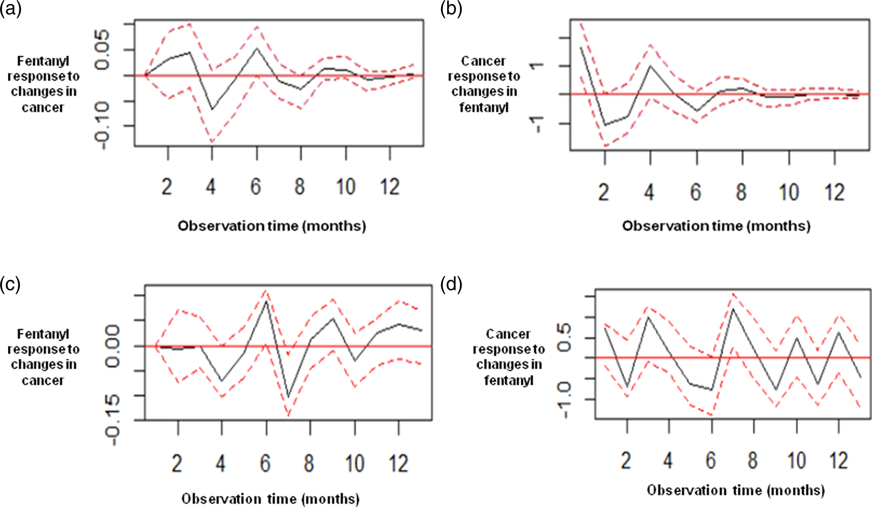

Figure 4(a) and (b) show another way to confirm the results of the impulse response functions, the forecasting error variance decomposition (FEVD), with the difference that FEDV does not show whether the reaction to a shock is positive or negative. FEDV indicate how much the future uncertainty of one time series is due to future shocks into the other time series. For both models, VAR (2) and VAR (11), the variability in dependent variables are mainly lagged by their own variance.

Figure 4.

Forecasting error variance decomposition (FEVD). (a) Results from the VAR (2) model. (b) Results from the VAR (11) model. FEVD determine how much of the variability in dependent variable is lagged by its own variance and the proportion of variation explained by exogenous shocks to the other variables. For the VAR (2) and VAR (11) models, the variability in dependent variables are mainly lagged by their own variance.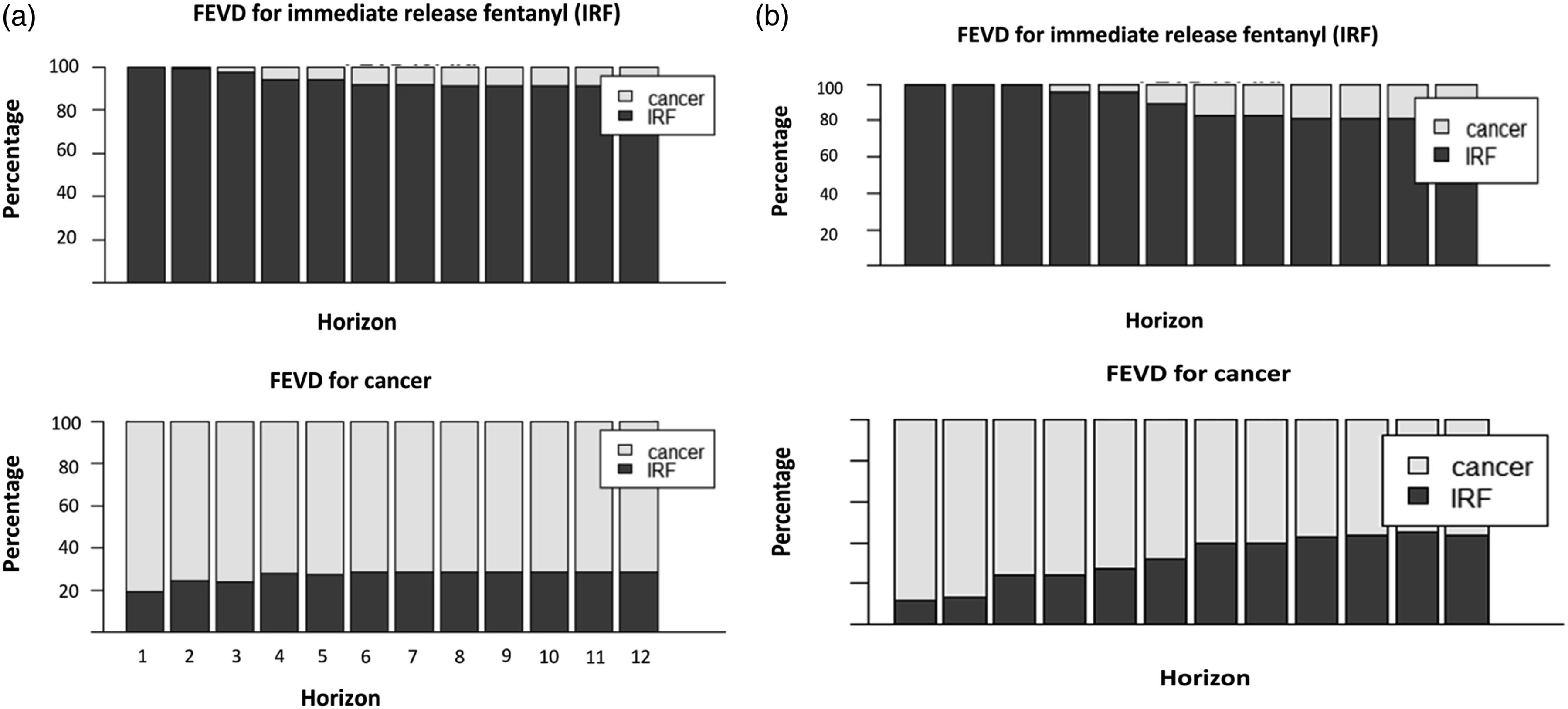

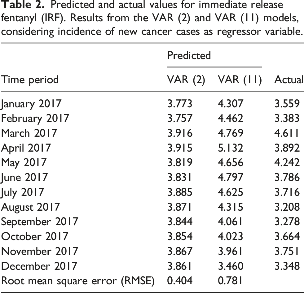
Table 2 contains IRF predicted incidences for the period covered by the test data (from January to December 2017) and the actual incidences observed. The RMSE for VAR (2) is lower than VAR (11), 0.4 and 0.7 respectively. Figure 2 represents the width of the 95% prediction interval against the horizon forecast. The forecasting power for VAR (2) and VAR (11), decrease from the 8^th observation predicted (Figure 5(a) and (b)).

Table 2.

Predicted and actual values for immediate release fentanyl (IRF). Results from the VAR (2) and VAR (11) models, considering incidence of new cancer cases as regressor variable.

Time period	Predicted		Actual
Time period	VAR (2)	VAR (11)	Actual
January 2017	3.773	4.307	3.559
February 2017	3.757	4.462	3.383
March 2017	3.916	4.769	4.611
April 2017	3.915	5.132	3.892
May 2017	3.819	4.656	4.242
June 2017	3.831	4.797	3.786
July 2017	3.885	4.625	3.716
August 2017	3.871	4.315	3.208
September 2017	3.844	4.061	3.278
October 2017	3.854	4.023	3.664
November 2017	3.867	3.961	3.751
December 2017	3.861	3.460	3.348
Root mean square error (RMSE)	0.404	0.781

Figure 5.

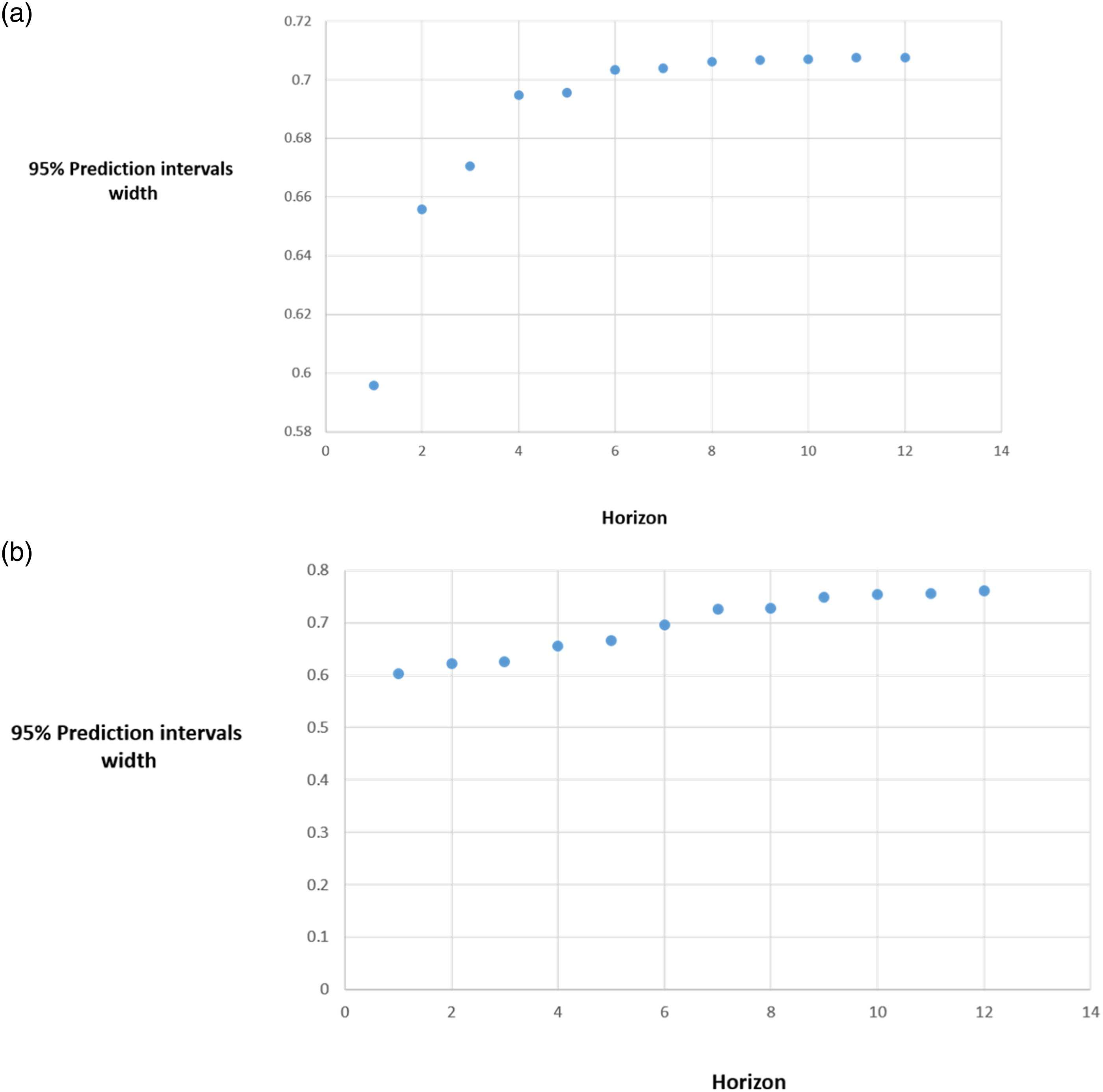
Forecasting accuracy for immediate release fentanyl. Width of the 95% prediction interval as a function of the forecast horizon. (a) Results from the VAR (2) model. (b) Results from the VAR (11) model. The y axis represents the width of the 95% prediction interval for monthly incidence of immediate release fentanyl use considering cancer incidence as regressor variable. The x axis charts the number of forecast observations or months in the future. The plots show width of the 95% prediction interval increases as the forecast horizon increases. For the VAR (2) and VAR (11) models, the prediction interval is constant from the 8th observation predicted, that is, from the 8th month, the forecast accuracy is minimal.

Discussion

This article demonstrates the utility of VAR method in pharmacovigilance research, developing a stable model using the incidence of IRF use and its dynamic association with cancer incidence. Previous studies have reported the use of multivariate time series analysis in this field, mainly for modelling and forecasting antimicrobial use and its relationship with antimicrobial resistance.^31–34 Considering the stability, forecast accuracy and how far ahead the two estimated VAR models predict the future, a good applicability of this tool in determining factors related to IRF use is suggested. Nevertheless some points need to be discussed. Firstly the variables cancer and IRF were both incorporated to the model as endogenous variables assuming a bidirectional relationship between them and demonstrating then bidirectional Granger causality. Despite the increase in IRF use does not imply an increase in cancer disease in a clinical sense, the incidences estimates were based on the diagnosis codes and prescriptions registered in BIFAP. In this type of data source, the indication might be registered in a time window pre and post IRF prescription. The fact that IRF granger cause cancer, should be interpreted as higher registries of IRF prescriptions in BIFAP, predict higher registries of oncology codes.

Regarding the impulse response, it is well known that its dynamic properties may depend critically on the order of the VAR model fitted to the data, as observed in our study. Parsimonius lag order selection criteria, may produce impulse response estimates that are more accurate at least at short horizon. In contrast, parsimonius lag order selection criteria may fail to capture complicated dynamics of impulse response functions, particularly at larger horizons.³⁵

According to the RMSE of the test data, the VAR (2) model seems to be slightly more accurate than the VAR (11). Nevertheless predicted and actual values for IRF use are closed for both models, VAR (2) and VAR (11) and differences were not relevant in terms of incidence. Based on RMSE and the parsimony principle of choosing the simplest scientific explanation that fits the evidence, VAR (2) might be preferable.

Finally the analysis showed a strong and linear correlation between cancer and IRF use, in spite of a previous study performed in BIFAP during the same study period reporting a 30% of newly IRF prescribed, without a register of cancer in their clinical record.⁴ This percentage might not be relevant in terms of global IRF incidence, in order to demonstrate its correlation and dynamic association with cancer incidence. Therefore we could assume that the increase in IRF use observed last decade might be largely explained by the increase in the pathology for which is indicated.

Conclusion

This study demonstrates that using a robust and structured VAR modelling approach is able to estimate dynamics associations, involving IRF use and cancer incidence. Such information might be useful to put in context trends in drugs use and success of regulatory interventions, identifying enablers and barriers for implementation.

Strength and limitations

To our knowledge, this is the first study modelling and forecasting IRF use and its dynamic association with cancer incidence, using a robust methodology based on multivariate time-series analysis. Large, automated medical encounter databases, such as BIFAP, are valuable data sources for ecological studies on concerns that may affect medication use. Nevertheless there are also limitations to be considered. The study consisted of population included in BIFAP, which might limit the generalizability of the results outside the context of this study. IRF prescriptions in private centers were not included, although the risk of bias is minimal given the almost universal coverage of the NHS. Normally the specialist makes the first prescription and the patient is then followed by the primary care physician, therefore is captured in BIFAP. We could not verify that the prescribed IRF were actually taken, which is much less of a concern for this study given our focus on IRF prescribing, rather than medication consumption. One potential limitation would be the potential error in the assessment of cancer outcome. However validity of cancer diagnoses in BIFAP database has been shown to be high³⁶ and this study was only based in registering codes, which decreases potential bias.

Granger causality should not be over-interpreted as truly causal. It can be stated as if the prediction of one time series is improved by incorporating the knowledge of a second time series, then the latter is said to have a causal influence on the first.³⁷

Conclusions of an ecological design from the results of aggregate data, should not be inferred about individuals. Any association observed between variables at the group level, does not necessarily mean that the same association exists for any given individual selected from the group.

Despite the aforementioned limitations, analyzing drug utilization and its dynamic association with the indication for its use in BIFAP, provides valuable information in order to guide future regulatory actions and rational use policy.

Supplemental Material

Supplemental Material - Dynamic relationship among immediate release fentanyl use and cancer incidence: A multivariate time-series analysis using vector autoregressive models

Supplemental Material for Dynamic relationship among immediate release fentanyl use and cancer incidence: A multivariate time-series analysis using vector autoregressive models by Diana González-Bermejo, Belén Castillo-Cano, Alfonso Rodríguez-Pascual, Pilar Rayón-Iglesias, Dolores Montero-Corominas and Consuelo Huerta-Álvarez in Journal of Research Methods in Medicine & Health Sciences

Footnotes

Acknowledgements

The authors would like to acknowledge the excellent collaboration of the primary care general practitioners and pediatricians, and the support of the regional authorities participating in the database (Aragón, Asturias, Canarias, Cantabria, Castilla y León, Castilla la Mancha, La Rioja, Madrid, Murcia, Navarra).

Declaration of conflicting interests

The author(s) declared no potential conflicts of interest with respect to the research, authorship, and/or publication of this article.

Funding

The author(s) disclosed receipt of the following financial support for the research, authorship, and/or publication of this article: The Spanish Database for Pharmacoepidemiology Research in Primary Care (BIFAP) is fully financed by the Spanish Agency of Medicine and Medical Devices (AEMPS).

Disclaimer

This document expresses the opinion of the authors of the paper and may not be understood or quoted as being made on behalf of or reflecting the position of the Spanish Agency of Medicine and Medical Devices or its committees or working parties.

Ethical statement

ORCID iD

Consuelo Huerta-Alvarez

Supplemental Material

Supplemental material for this article is available online.

References

Hastie

Gilson

Maurer

, et al. An examination of global and regional opioid consumption trends 1980–2011. J Pain Palliat Care Pharmacother 2014; 28(3): 259–275.

Hider-Mlynarz

Cavalié

Maison

. Trends in analgesic consumption in France over the last 10 years and comparison of patterns across Europe. Br J Clin Pharmacol 2018; 84: 1324–1334.

Bosetti

Santucci

Radrezza

, et al. Trends in the consumption of opioids for the treatment of severe pain in Europe, 1990–2016. Eur J Pain 2019; 23(4): 697–707.

González-Bermejo

Rayón-Iglesias

Rodríguez-Pascual

, et al. Drug utilization study on immediate release fentanyl in Spain. Prevalence, incidence, and indication. Pharmacoepidemiol Drug Saf 2021; 30(3): 371–378.

Summary of product characteristics for immediate release fentanyl. Spanish Agency of Medicines and Medical Devices. https://cima.aemps.es/cima/publico/home.html. Accessed 27 February, 2021.

Rosenblum

Marsch

Joseph

, et al. Opioids and the treatment of chronic pain: controversies current status and future directions. Exp Clin Psychopharmacol 2008; 16(5): 405–416.

Portenoy

Messina

Xie

, et al. Fentanyl buccal tablet (FBT) for relief of breakthrough pain in opioid-treated patients with chronic low back pain: a randomized, placebo-controlled study. Curr Med Res Opin 2007; 23: 223–233.

Simpson

Messina

Xie

, et al. Fentanyl buccal tablet for the relief of breakthrough pain in opioid-tolerant adult patients with chronic neuropathic pain: a multicenter randomized, double blind, placebo-controlled study. Clin Therapeut 2007; 29: 588–601.

Ashburn

Slevin

Messina

, et al. The efficacy and safety of fentanyl buccal tablet compared with immediate-release oxycodone for the management of breakthrough pain in opioid-tolerant patients with chronic pain. Anesth Analg 2011; 112: 693–702.

10.

Farrar

Messina

Xie

, et al. A novel 12-week study, with three randomized, double-blind placebo-controlled periods to evaluate fentanyl buccal tablets for the relief of breakthrough pain in opioid-tolerant patients with non cancer-related chronic pain. Pain Med 2010; 11: 1313–1327.

11.

Fine

Messina

Xie

, et al. Long-term safety and tolerability of fentanyl buccal tablet for the treatment of breakthrough pain in opioid-tolerant patients with chronic pain: an 18-month study. J Pain Symptom Manag. 2010; 40(5): 747–760.

12.

European Medicines Agency . Effentora: withdrawal of the application to change the marketing authorization. Report on July 2013: EMA/447220/2013, EMEA/H/C/000833/II/18. https://www.ema.europa.eu/en/documents/medicine-qa/questions-answers-withdrawal-application-change-marketing-authorisation-effentora-fentanyl_es.pdf. Accesed 12 June 2023.

13.

Lütkepohl

. New introduction to multiple time-series analysis. Berlin, Heidelberg: Springer-Verlag, 2005.

14.

Bose

Hravnak

Sereika

. Vector autoregressive models and granger causality in time series analysis in nursing research: dynamic changes among vital signs prior to cardiorespiratory instability events as an example. Nurs Res 2017; 66(1): 12–19.

15.

Pfaff

. VAR, SVAR and SVEC models: implementation with R package vars. J Stat Softw. 2008; 27(4): 1–32.

16.

Maciá Martínez

Gil

Huerta

, et al. Base de datos para la investigación farmacoepidemiológica en atención primaria (BIFAP): a data resource for pharmacoepidemiology in Spain. Pharmacoepidemiol Drug Saf 2020; 29(10): 1236–1245.

17.

Requena

Huerta

Gardarsdottir

, et al. Hip/femur fractures associated with the use of benzodiazepines (anxiolytics, hypnotics and related drugs): a methodological approach to assess consistencies across databases from the PROTECT-EU project. Pharmacoepidemiol Drug Saf 2016; 25(Suppl 1): 66–78.

18.

WONCA . Classification in primary care version 2 in Spanish. https://www.semfyc.es/formacion-y-recursos/biblioteca-virtual/clasificacion-ciap-2/, Accessed 12 June 2023.

19.

World Health International . Classification of diseases. 9th ed. https://eciemaps.mscbs.gob.es (Accessed 12 June 2023).

20.

WHO Collaborating Centre for Drug Statistcs Methodology . ATC/DDD index, 2019, https://www.whocc.no/atc_ddd_index/(Accessed 27 November, 2020).

21.

Vrieze

. Model selection and psychological theory: a discussion of the differences between the akaike information criterion (AIC) and the bayesian information criterion (BIC). Psychol Methods 2012; 17(2): 228–243.

22.

Hamilton

. Time series analysis. Princeton, NJ: Priceston University Press, 1994.

23.

Granger

CWJ

. Investigating causal relations by econometric models and cross-spectral methods. Econometrica 1969; 37: 424–438.

24.

Nájera-Salmerón

. Relationship in the cryptocurrencies price behavior: an econometric analysis through VAR and VEC models. Estocástica: Finanzas Y Riesgo 2019; 9(1): 33–61.

25.

Armstrong

Collopy

. Error measures for generalizing about forecasting methods: empirical comparisons. Int J Forecast 1992; 8(1): 69–80.

26.

Hyndman

and Athanasopoulos

. Forecasting: principles and practice. 2nd ed. Melbourne, Australia: OTexts, 2018.

27.

Enders

. Applied econometric time series. Chicago: Wiley, 2004.

28.

Pfaff

. VAR, SVAR and SVEC Models: implementation within R package vars. J Stat Softw 2008; 27(4): 1–32.

29.

Lütkepohl

. New introduction to multiple time series analyis. Berlin: Springer 2007.

30.

Tesay

. Multivariate time series analysis: with R and financial applications (wiley series in probability and statistics). Chicago: Wiley, 2013.

31.

Tóth

Fésűs

Kungler-Gorácz

, et al. Utilization of vector autoregressive and linear transfer models to follow up the antibiotic resistance spiral in gram-negative bacteria from cephalosporin consumption to colistin resistance. Clin Infect Dis 2019; 69(8): 1410–1421.

32.

Lawes

López-Lozano

Nebot

, et al. Turning the tide or riding the waves? Impacts of antibiotic stewardship and infection control on MRSA strain dynamics in a Scottish region over 16 years: non-linear time series analysis. BMJ Open 2015; 5(3): e006596.

33.

López-Lozano

Monnet

Yagüe

, et al. Modelling and forecasting antimicrobial resistance and its dynamic relationship to antimicrobial use: a time series analysis. Int J Antimicrob Agents 2000; 14(1): 21–31.

34.

Aldeyab

Monnet

López-Lozano

, et al. Modelling the impact of antibiotic use and infection control practices on the incidence of hospital-acquired methicillin-resistant Staphylococcus aureus: a time-series analysis. J Antimicrob Chemother 2008; 62(3): 593–600.

35.

Ivanov

Kilian

. A practitioner’s guide to lag order selection for VAR impulse response analysis. Stud Nonlinear Dyn Econom 2005; 9(1). Article 2.

36.

Gil

Rodríguez-Miguel

Montoya-Catalá

, et al. Validation study of colorectal cancer diagnosis in the Spanish primary care database, BIFAP. Pharmacoepidemiol Drug Saf 2019; 28(2): 209–216.

37.

Eichler

. Causal inference with multiple time series: principles and problems. Philos Trans A Math Phys Eng Sci. 2013; 371 (1997): 20110613. DOI: 10.1098/rsta.2011.0613.

Supplementary Material

Please find the following supplemental material available below.

For Open Access articles published under a Creative Commons License, all supplemental material carries the same license as the article it is associated with.

For non-Open Access articles published, all supplemental material carries a non-exclusive license, and permission requests for re-use of supplemental material or any part of supplemental material shall be sent directly to the copyright owner as specified in the copyright notice associated with the article.

0.00 MB

0.64 MB