Sage Journals: Discover world-class research

Abstract

Psychological researchers usually make sense of regression models by interpreting coefficient estimates directly. This works well enough for simple linear models but is challenging for more complex models with, for example, categorical variables, interactions, nonlinearities, or hierarchical structures. Here, we introduce an alternative approach to making sense of statistical models. The central idea is to abstract away from the mechanics of estimation and to treat models as “counterfactual prediction machines,” which are subsequently queried to estimate quantities and conduct tests that matter substantively. This workflow is model-agnostic; it can be applied in consistent fashion to draw inferences from a wide range of models. We illustrate how to implement this workflow with the marginaleffects package, which supports more than 100 different classes of models in R and Python, and present two worked examples. These examples show how the workflow can be applied across designs (e.g., observational studies, randomized experiments) to answer different research questions (e.g., about associations, causal effects, effect heterogeneity) while facing various challenges (e.g., controlling for confounders in a flexible manner, modeling ordinal outcomes, and interpreting nonlinear models).

Keywords

regression linear modeling nonlinear modeling marginal effects open data open materials

Researchers often test their theories or explore their data by fitting regression models, including varieties such as multilevel models or generalized linear models. How can one make sense of the results of such models? The standard approach is to focus on coefficients and use them to gauge the association between the focal predictor(s) and some outcome. In the simplest linear models, this is easy enough: A coefficient estimate shows how the outcome can be expected to change when the associated predictor increases by 1 unit.

The real strength of regression modeling, however, lies in its ability to move beyond simple bivariate associations to support complex analyses that account for interactions, nonlinearities, hierarchical structures, and other complications. Unfortunately, when models become more complex—and thus arguably more realistic—the direct interpretation of coefficients also becomes more complex, and researchers must fall back on heuristics or cumbersome data transformations. These strategies can be confusing and error-prone, and the statistical estimates that they generate do not always answer the questions that researchers actually care about.

To illustrate these challenges, in this article, we begin by discussing a few common scenarios in which interpreting model results can be difficult (see Coefficients Can Confuse). We then introduce a different perspective in which models are treated as “counterfactual prediction machines” that generate quantities relevant to substantive research questions (see Models as Prediction Machines). This results in a simple yet powerful workflow. First, one has to settle on a target quantity—or estimand (Lundberg et al., 2021)—of interest, which represents the analysis goal (i.e., targets). An estimand can be descriptive (e.g., estimating the prevalence of a characteristic), associational (e.g., quantifying how strongly two characteristics are associated), or causal (e.g., quantifying how strongly one characteristic affects another). Once a target quantity is chosen, it can be estimated and assessed using, for example, null hypothesis and equivalence tests (i.e., tests). In practice, these steps can be implemented with the open-source marginaleffects package for R and Python (i.e., tools; Arel-Bundock et al., 2024). Finally, we illustrate how to conduct such analyses in two worked examples, showcasing the strengths of this approach. It provides a consistent way to interpret statistical models across designs and research questions, even in challenging scenarios, such as flexible models including nonlinearities and interactions. In that manner, it enables researchers to implement more challenging model classes, such as ordinal models, without losing the ability to interpret them coherently.

This alternative workflow is not our invention—some researchers across fields, including psychology, already calculate and report the target quantities we discuss, using both “manual” custom procedures or various statistical packages. For example, the commercial software Stata provides postestimation capabilities that are routinely used in other social sciences. The purpose of this article is to highlight the benefits of an estimand-centered approach to making sense of statistical models and provide an accessible and hands-on introduction for researchers who were trained in a different tradition and seek to expand their toolbox.

Coefficients Can Confuse

To set the scene, we present common scenarios in which the interpretation of model coefficients can get more complicated.

Interactions

Researchers in psychology often use regression models to trace how an association varies across strata of the sample or show that the effect of a treatment is modified by a moderator. One popular strategy to study these forms of heterogeneity is to fit a regression equation with multiplicative interactions. When a model includes interaction terms, the association between the focal predictor and the outcome is no longer captured by a single coefficient but rather by a combination of coefficients. Focusing on individual coefficients can result in erroneous or incomplete interpretations, and there is some evidence that researchers do indeed fall into this trap (Hayes et al., 2012). Indeed, many researchers have mistakenly interpreted a coefficient capturing a conditional effect (the effect for individuals with specific values on a third variable) as if it were the main effect in an analysis of variance (the unweighted average across individuals with different values on a third variable).

Nonlinearity in the predictors

Another important application of regression modeling is to study nonlinear relationships between predictors and outcomes. For example, analysts who wish to control for a covariate without making overly strong functional form assumptions may fit a model with polynomials or splines. However, the parameters of polynomial models create the same interpretation trap as interaction models: They must be interpreted in combination. Matters only get worse for splines, which produce multiple coefficients for a single covariate, and those coefficients now refer to synthetic variables derived from that covariate in a rather opaque manner.

Nonlinear link functions

For discrete outcomes, or continuous outcomes with skewed distributions, researchers routinely fit generalized linear models with some (nonlinear) link function, such as logistic, probit, Poisson, or log-linear models. Here, the link function adds further complications to the interpretation of coefficients. Consider a logistic regression model fit to a binary outcome. Each of the coefficient estimates returned by that model is expressed as a log odds ratio, that is, as the natural logarithm of a ratio of ratios of probabilities. But studies in psychology and behavioral economics show that people already struggle to interpret even the simplest of probabilities (Nickerson, 2004). For clinicians, researchers, and the lay public, drawing insight from a ratio of ratios of probabilities is surely much harder (e.g., Norton et al., 2024). In some contexts, logit coefficients may even fail to map onto quantities of interest altogether (Halvorson et al., 2022).¹

Another complexity is added when interactions are investigated in models with nonlinear link functions. Here, contemporary recommendations (McCabe et al., 2022; Mize, 2019) emphasize that the coefficient of the product term no longer provides a suitable way to evaluate the magnitude or even just the existence of an interaction. Put simply, although it is often crucial for analysts to account for nonlinearities or discrete outcomes, the regression models that achieve this goal produce coefficient estimates that are difficult to interpret on their own.

Categorical predictors

When models include categorical predictors representing different groups, multiple coding schemes may be used (e.g., dummy, polynomial, Helmert, or deviation coding). The basic idea is to transform the raw data before fitting the model so that the resulting coefficient estimates relate to the comparisons of interest (e.g., each group vs. one reference group, each group vs. the grand mean). These data transformations are, in a sense, bespoke and single-use. They need to be tailored to the specific research question, and they often require refitting the model when the question changes (e.g., when a different group contrast is supposed to be tested against zero). Moreover, custom contrast codings can generate collateral damage, such as hard-to-track errors during data wrangling.

The Table 2 fallacy

When it comes to interactions and nonlinearities, coefficients may be misinterpreted in cases in which a correct interpretation is possible. In some situations, however, attempts to interpret some coefficients directly should be discouraged altogether. To see why, consider that one common goal of regression modeling is to control for confounders that prevent one from interpreting the association between a potential cause and an outcome in causal terms. But when a model includes many coefficients, researchers are tempted to interpret them all—including those associated with control variables. In doing so, they would commit what Westreich and Greenland (2013) called the “Table 2 fallacy.” Indeed, from a causal-inference perspective, interpreting the coefficients of control variables is often incoherent (Keele et al., 2020).

To see why, imagine a model built to investigate the causal effect of the number of books in the household on children’s reading scores. Obviously, socioeconomic status (SES) can confound the relationship of interest because it likely affects both the number of books in a household and the reading scores of the residents (number of books ← SES → reading score). In that context, it is important for the regression model to control for SES, and the resulting model will return a coefficient for SES. However, that coefficient does not have a straightforward interpretation because the model also includes number of books, which is causally downstream of SES (SES → number of books → reading score). If the goal is to estimate the effect of SES on reading scores, then controlling for the number of books is inappropriate because it removes part of the effect of interest (overcontrol bias). As a result, the model is appropriate to estimate the effect of number of books but inappropriate to estimate the effect of SES. Moreover, controlling for the number of books may actually induce new noncausal associations between SES and reading scores via third variables (collider bias) so that an interpretation in the spirit of the “direct effect” in the context of a mediation analysis is usually not warranted either (Rohrer, 2018; Rohrer et al., 2022).²

Reporting regression coefficients may still have benefits. For example, a table of regression coefficients may make it easier to figure out the precise model specification (in particular if no regression equation is reported, as is often the case in psychology), and it may even enable readers to catch certain types of errors. The problem of the Table 2 fallacy chiefly arises when coefficients are substantively interpreted, which some researchers seem to do habitually whenever such a table is presented.

Models as Prediction Machines

In summary, interpreting model coefficients directly is a difficult and error-prone business. But what would be an alternative? How else can one interpret statistical models?

A good starting point is the realization that often, model coefficients are not the logical end of a model; they are merely the statistical machinery that allows the model to achieve its goal. That goal is straightforward: to predict the outcome that one should expect for an individual or unit given some characteristics and to quantify the uncertainty of that prediction.³ The core of our alternative approach thus involves thinking of the model as a prediction machine and transforming the quantities it produces to answer substantive research questions.

The workflow we recommend has three steps. First, the analyst fits a statistical (or machine learning) model. This model should be designed to meet domain-specific requirements. For example, it could be set up to control for known confounders, capture salient features of the data-generating process, maximize predictive accuracy while avoiding overfitting, or account for nonlinearities and heterogeneity. Researchers may also fit multiple models and apply a model-selection procedure before settling on a model with which they want to continue. Second, they use the model to make predictions for the outcome variable given specific values of predictors. These predictions can be made for the actual observations in the data set (i.e., “fitted values”), or researchers can manipulate the predictor values to produce so-called “counterfactual predictions” (“What outcome would we expect to observe if things were different?”). Third, the analysts summarize and combine predictions to obtain an estimate of the statistical quantity—the estimand—that actually answers their research questions. Below, we provide guidance on Steps 2 and 3 because these are the points at which the workflow we recommend diverges from standard training. Figure 1 provides an overview of the workflow.

Fig. 1.

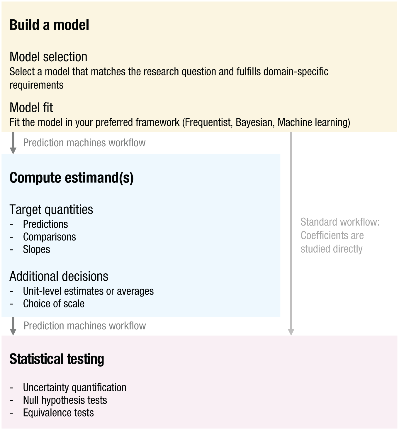
Overview of the workflow in which models are treated as prediction machines. Researchers build a model, use the model to compute meaningful target quantities, and subsequently conduct tests on these quantities. In contrast, in the standard workflow, researchers directly interpret and test the model coefficients.

A big advantage of this approach is that it is model-agnostic. Interpretation works the same regardless of whether the model is linear, generalized linear, or generalized additive; whether it includes a multilevel structure; whether it contains interactions and/or splines; or whether it is estimated using a Bayesian or frequentist approach. The workflow can also be applied to machine-learning models, in which case, it aligns closely with ideas from the interpretable machine-learning tradition that aims to summarize model behavior in a model-agnostic manner (Molnar, 2020). Across models, the software commands that analysts need to execute stay the same, which greatly facilitates the exploration of model specifications to check the robustness of findings. Other smaller perks include that one does not need to perform preestimation transformations, such as centering or contrast coding. For categorical predictors, for example, one can simply include them “as is” and then use postestimation commands to calculate any contrast of interest.

Most importantly, this workflow unburdens researchers from the cognitive load of reverse-engineering the mechanics of their models. This frees up some headspace to focus on other aspects, such as ensuring that the statistical quantities researchers report actually map onto the theory they hope to test (i.e., defining a clear estimand; Lundberg et al., 2021) and understanding the necessary assumptions that buttress their results (e.g., concerns regarding construct or external validity, Esterling et al., 2025; or regarding internal validity, Rohrer, 2018).

Workflow: Targets, Tests, and Tools

Target quantities

The first step of any statistical analysis should be to state one’s research question explicitly and to specify exactly which target quantity—which estimand—can shed light on this question (Lundberg et al., 2021). Consider a regression model that predicts life satisfaction from people’s age, gender, and income (including nonlinear effects and interactions between the predictors).⁴ What can one actually do with that model? What research questions can one address with its help, and what quantities should one extract to answer those questions? Specifying the target quantity involves three parts: the quantity of interest (predictions, comparisons, slopes), the unit of interest (individuals, averages across individuals, or a target population), and the scale of interest (e.g., the link scale or the response scale, also called “natural scale”). Some of the resulting combinations are referred to as “marginal effects” in the literature, that is, comparisons and slopes on the natural scale.⁵ However, in the workflow we champion, marginal effects are only a subset of the target quantities that may be of interest, and so we focus on the general logic of target-quantity construction rather than individual named effects.⁶

Predictions

The first (and simplest) question one can ask is the following: What is the model’s expected outcome for an individual with given characteristics? To answer it, one feeds particular values of the predictors to a model and gets a prediction in return. Consider our regression model predicting life satisfaction from age, gender, and income. By fixing the predictors to specific values, one learns that the fitted model expects a 35-year-old woman who earns 20,000€ per year to score a 7.65 on the life-satisfaction scale (range = 0–10). In Figure 2, this prediction is marked by the blue dot to the left, which sits on a black curve that represents the predicted life satisfaction for 35-year-old women across different levels of income. This expectation—or prediction—is the most basic statistical quantity that analysts can target in a regression context.

Fig. 2.

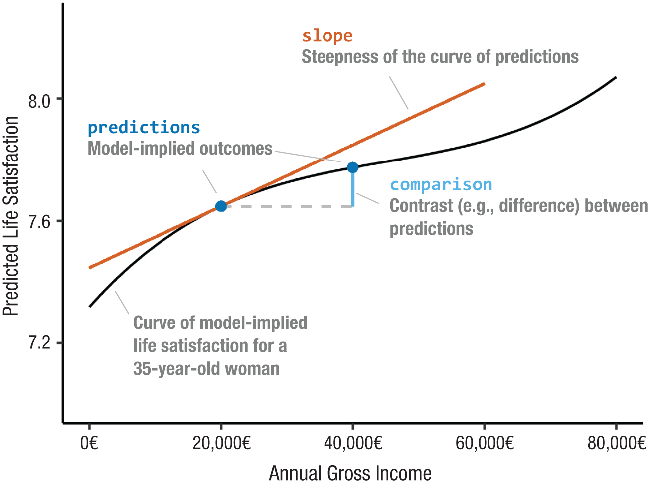
Results from a regression model predicting life satisfaction from age, gender, and income in data from the German Socio-Economic Panel Study. The black line shows predicted life satisfaction for a 35-year-old woman across different levels of income. The blue dots mark two predictions: predicted life satisfaction at 20,000€ and predicted life satisfaction at 40,000€. The light-blue line marks the comparison between these two predictions. The orange-red line visualizes the slope, that is, the instantaneous change in predicted life satisfaction with income for an income of 20,000€.

Comparisons

Going one step further, analysts may be interested in the association between one (or more) predictor(s) and the outcome, or in the effect of a treatment. They may wish to know how the outcome is expected to change when predictors change. To answer this question, all one has to do is make predictions for two hypothetical (i.e., counterfactual) individuals and then compare the two computed quantities. Consider two individual profiles and their associated model-based predictions: (a) 35-year-old woman with an income of 20,000€, predicted life satisfaction of 7.65 (Fig. 2, left blue dot), and (b) 35-year-old woman with an income of 40,000€, predicted life satisfaction of 7.77 (Fig. 2, right blue dot).

In this example, the only difference between the two individuals is their income; all other variables are held at the same values. To quantify the estimated effect of the income intervention, or the estimated association between income and life satisfaction, all one has to do is compare the two predicted outcomes.

To do this, one can use a variety of functions. The most obvious approach is to take a simple difference: 7.77 – 7.65 = 0.13. For a 35-year-old woman, our model expects that increasing income by 20,000€ is associated with an increase of 0.13 on the life-satisfaction scale (marked with a vertical light-blue line in Fig. 2). But one could also take the ratio of the two predicted outcomes: 7.77 / 7.65 = 1.02. For a 35-year-old woman, our model expects that increasing income by 20,000€ is associated with an increase in life satisfaction of about 2%. Admittedly, the ratio is a bit of an uncommon choice here,⁷ but for binary outcomes, differences and ratios are routinely reported as “risk differences” and “risk ratios” (see section below: Quantification on Different Scales).

Comparisons between predictions are useful when the analysts’ goal is to study associations or to make causal claims. They can always be thought of as a measure of conditional association, holding control variables constant. In some cases, when additional identification assumptions are met, they can also be interpreted causally, as the contrast between two potential states of the world. Determining whether a causal interpretation is warranted requires careful consideration of identification assumptions (for an introduction in psychology, see Rohrer, 2018). In our running example, omitted confounders, such as health, education, or personality, likely prevent a causal interpretation of the relationship between income and life satisfaction.

Slopes

The counterfactual comparison above focused on two (discrete) income levels to see what our model says about the relationship between income and life satisfaction. But income may be thought of as a continuous variable, so one may wonder the following: For a 35-year-old woman, how steeply does life satisfaction rise with income at, for example, 20,000€? What is the slope of the prediction curve; what is the rate of change in life satisfaction when income goes up by an infinitesimally small amount, according to our model? When one computes this quantity, the model show that for the woman under consideration, the slope is approximately 0.00001 life-satisfaction points per €, or using a slightly more reasonable unit, 0.01 points per 1,000€. In Figure 2, this slope is represented by the orange-red line, which is the tangent that touches the prediction curve at the income level of interest. This slope can be interpreted as an estimate of the strength of conditional association between a continuous predictor and the outcome.

Individuals, averages, and target populations

So far, we have discussed target quantities—predictions, comparisons, and slopes—for a single individual with specific predictor values: a 35-year-old woman with 20,000€ in income. In principle, one can calculate target quantities for every imaginable combination of predictor values, including some that may not be covered by the data at all and some that may be nonsensical. More reasonably, one may calculate target quantities for combinations of particular interest. This would involve calculating target quantities for a hypothetical individual whose characteristics are average (e.g., a person of average age with the average income) or target quantities for hypothetical individuals whose characteristics take on predefined “representative” values (e.g., the ages of 20, 30, 40, 50, and 60).

More generally, one need not limit the analysis to a handful of individuals. Target quantities may be calculated for every row of the observed data set. Such unit-specific estimates can then be aggregated to produce summary quantities of broader interest. Averaging can also be performed for specific subgroups (e.g., women, college graduates) or using weights, to target a population that is not perfectly represented by the sample.

This empowers researchers to compute a wealth of different target quantities to summarize and contrast model predictions for different units. Some of these target quantities have received special attention in the literature. For example, one can estimate the average treatment effect (ATE) of a binary predictor by computing counterfactual comparisons for every individual in the observed data and taking the average of those estimates. Or one can compute the ATE on the treated in the same way but by considering only the subset of observed individuals who actually received the treatment (Arel-Bundock, 2026, Chapter 8). This approach is often called “g-computation” or “parametric g-formula” in epidemiology and statistics (Chatton & Rohrer, 2024).

Another popular set of target quantities in the social and behavioral sciences were labeled by Williams (2012) as marginal effect at the mean (MEM), marginal effects at representative values (MERs), and average marginal effect (AME). In our terminology, these would correspond to (a) the slope for a hypothetical individual whose characteristics are average (MEM), (b) the slope for hypothetical individuals whose characteristics are representative (MERs), and (c) the average of all slopes computed for each individual in the observed data set (AME).⁸

As we demonstrate below, all of these target quantities are trivial to compute using the marginaleffects package for R and Python. We note that individual regression coefficients can correspond to specific target quantities of interest in certain simple scenarios (e.g., in a simple linear regression model, a coefficient may correspond to the AME). However, this correspondence usually breaks in more complex scenarios (e.g., in nonlinear models), and so estimating a clearly specified target quantity provides a more general solution than interpreting regression coefficients.

Quantification on different scales

Above, we reported quantities expressed on the actual outcome scale—points on a life-satisfaction scale. Depending on the type of model used, other outcome scales may also be sensible. For example, in a binary logistic regression, the model expresses the log-odds of a binary outcome as a linear function of the predictors. One could therefore compute quantities of interest on this log-odds scale, which happens to be the scale on which coefficients are usually displayed by default. Alternatively, it is possible to transform the log-odds into odds ratios, another common way to summarize effects. Finally, because odds are unfamiliar to most audiences—except perhaps statisticians and gamblers—it may be more intuitive to present results on the “original” response scale (also called the natural scale), which for the case of a binary outcome, corresponds to probabilities.

Figure 3 illustrates different scales in a logistic-regression context. The x-axis shows values on the log-odds scale (the link scale), and the y-axis shows the corresponding probabilities (the response scale). Two predictions are marked with blue dots. The counterfactual comparison of these two predictions can be quantified in a variety of ways, depending on whether one reports them on the log-odds scale or the probability scale and whether one takes a simple difference or instead calculates some ratio, resulting in four combinations: the log-odds difference, the odds ratio, the risk difference, and the risk ratio.

Fig. 3.

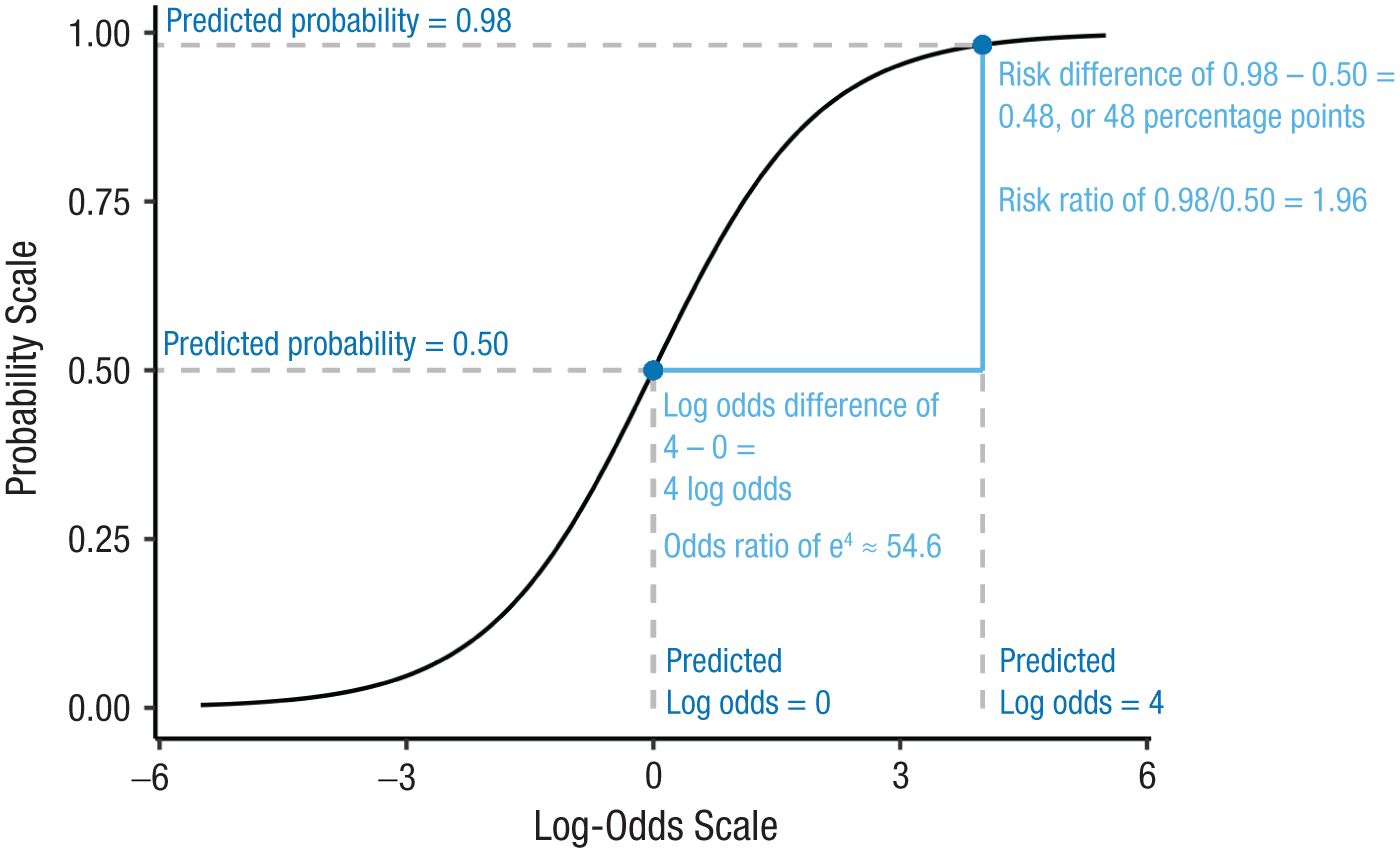
Mapping between the log-odds scale (the link scale underlying binary logistic regression) and the probability scale (probability of outcome = 1, response scale). The two blue dots mark two predictions that a binary logistic model may return. The comparison between these two predictions can be expressed in different ways, depending on which scale one chooses (log-odds vs. probability) and how the predictions are contrasted (difference vs. ratio).

Notice that results may look quite different on different scales even when they refer to the same model and thus simply reexpress the same findings in different terms. For example, a risk ratio of 0.06 / 0.03 = 2 may sound more impressive than the corresponding risk difference of 0.06 − 0.03 = 0.03. This becomes all the more salient when interactions are of interest because the same interaction expressed on different scales varies in apparent magnitude and can even change sign (Rohrer & Arslan, 2021).

Tests

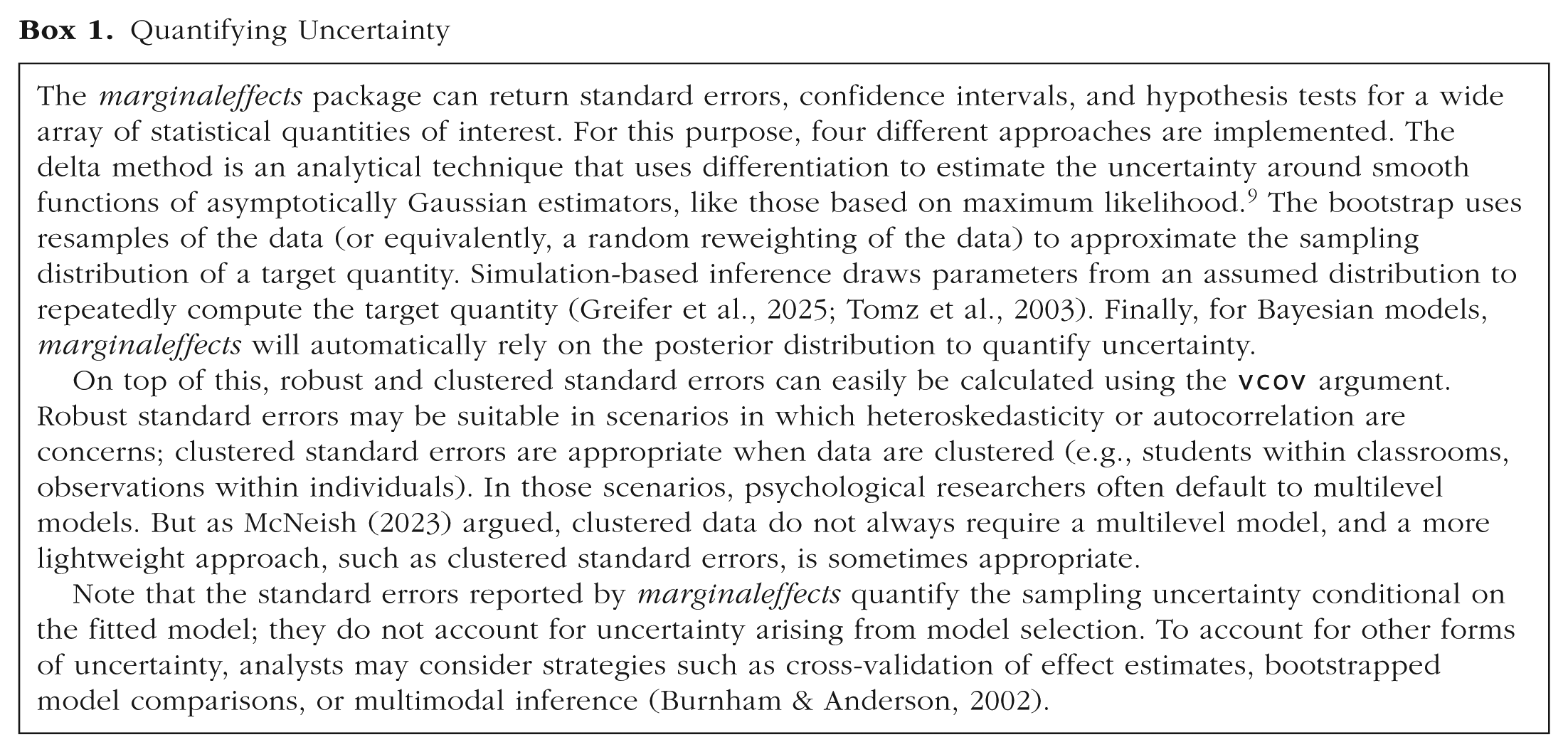
Researchers focusing on coefficients are often interested in the uncertainty associated with those coefficients and in whether they are statistically significantly different from zero. However, when focusing on target quantities instead, the significance of individual coefficients is of little interest. Rather, researchers may want to measure the uncertainty associated with their target quantities (see Box 1), and they may also wish to subject these quantities to various statistical-testing procedures, such as testing whether they should reject a null hypothesis (typically: no difference/association/effect) given a certain model and set of assumptions. In that manner, the statistical test conducted directly refers to the metric the analyst has determined to be substantively meaningful.

Box 1.

Quantifying Uncertainty

The marginaleffects package can return standard errors, confidence intervals, and hypothesis tests for a wide array of statistical quantities of interest. For this purpose, four different approaches are implemented. The delta method is an analytical technique that uses differentiation to estimate the uncertainty around smooth functions of asymptotically Gaussian estimators, like those based on maximum likelihood.⁹ The bootstrap uses resamples of the data (or equivalently, a random reweighting of the data) to approximate the sampling distribution of a target quantity. Simulation-based inference draws parameters from an assumed distribution to repeatedly compute the target quantity (Greifer et al., 2025; Tomz et al., 2003). Finally, for Bayesian models, marginaleffects will automatically rely on the posterior distribution to quantify uncertainty.On top of this, robust and clustered standard errors can easily be calculated using the vcov argument. Robust standard errors may be suitable in scenarios in which heteroskedasticity or autocorrelation are concerns; clustered standard errors are appropriate when data are clustered (e.g., students within classrooms, observations within individuals). In those scenarios, psychological researchers often default to multilevel models. But as McNeish (2023) argued, clustered data do not always require a multilevel model, and a more lightweight approach, such as clustered standard errors, is sometimes appropriate.Note that the standard errors reported by marginaleffects quantify the sampling uncertainty conditional on the fitted model; they do not account for uncertainty arising from model selection. To account for other forms of uncertainty, analysts may consider strategies such as cross-validation of effect estimates, bootstrapped model comparisons, or multimodal inference (Burnham & Anderson, 2002).

Importantly, null hypothesis tests are not limited to certain quantities—one can conduct them for predictions, counterfactual comparisons, slopes, or even complex (potentially nonlinear) functions of these quantities. They are also not limited to testing a null of zero. For example, one may want to test whether a prediction significantly differs from some meaningful value, such as an established cutoff. Or one may wish to test if two predictions differ from one another. This flexibility allows researchers to test a wide range of substantive hypotheses.

An equivalence test flips the logic of a null hypothesis test: Instead of asking whether one can reject a null of no effect, it asks whether one can reject the possibility that the size of effect is substantively meaningful (Lakens et al., 2018). Again, such tests can be applied to a variety of quantities.

Tools

To compute the targets and tests of interest, researchers need tools. The marginaleffects package for R and Python provides a comprehensive toolbox that allows researchers to implement the suggested model-agnostic framework in a simple and consistent manner (Arel-Bundock et al., 2024). The package supports more than 100 model types, including linear, generalized-linear, generalized-additive, multilevel, categorical-outcome, survival, Bayesian, and machine-learning models. For all of these models, a wide variety of quantities and tests can be easily calculated, relying on the exact same software commands regardless of the underlying prediction machine, that is, regardless of the precise model that was fitted.

The marginaleffects package also accommodates the needs of researchers who rely on more specialized analyses and workflows and provides functionality for Bayesian inference, factorial and conjoint experiments, contrasts, elasticities, interrupted time series, interval tests, inverse probability weighting, joint hypothesis tests, marginal means, matching, multiple imputation for missing data, and more.

All the functions in this package return “tidy” data that integrate smoothly with the broader R and Python ecosystems (Wickham, 2014), making it easy to visualize and summarize findings. The package is backed by extensive documentation and is actively being developed.¹⁰ Table 1 provides an overview of the most relevant functions and arguments, which are all showcased in the following examples.

Table 1.

Overview of Relevant Functions and Arguments of the marginaleffects Package

Function or argument	Explanation
predictions()	Outcome predicted by a supplied fitted model for every unit in the supplied data (default: data on which the model was fitted)
comparisons()	Predict the outcome at different regressor values and compare those predictions for every unit in the supplied dataSpecify the focal variables across which comparisons should be conducted with the variables argument
slopes()	Partial derivative of the regression equation with respect to a predictor of interest (supplied via the variables argument) for every unit in the supplied data
type =	Argument to indicate the scale on which target quantities should be computed, for example, “response”, “link”, “probs”
newdata =	Argument to supply predictor data for which target quantities will be computed
datagrid()	A convenient function to compute estimates, for example, “at the mean,” “at the median,” or at “representative values”
avg_predictions(), avg_comparisons(), avg_slopes()	Compute the respective unit-level target quantity and average across unitsWeights can be supplied with the wts argument
by =	Argument to generate subgroup averages of the target quantity
hypothesis =	Specify a linear or nonlinear null hypothesis test to be conducted on the target quantities
equivalence =	Specify bounds for an equivalence test (frequentist models) or the region of practical equivalence (Bayesian models)

Worked Examples

In this section, we present two worked examples that showcase the benefits of our recommended approach. Example 1 illustrates how to answer an associational research question: Do people in relationships say that friends matter less to them? We use data collected in a cross-sectional observational survey and fit both linear and ordinal regression models. We show how comparisons can easily be evaluated even when model complexity is increased by including splines and interactions. Example 2 shows how to answer a causal research question: Does sitting next to each other make it more likely that students befriend each other even if they are quite different from one another? We analyze data collected in a randomized field experiment using a Bayesian multilevel model. We also illustrate how to find out whether an effect is practically equivalent to a previously reported effect size and how to evaluate moderation claims. All data and analysis code, including a downloadable replication package, are available at https://j-rohrer.github.io/marginal-psych.

Example 1: relationship status and the importance of friends

It is a common complaint that people who enter a relationship start to neglect their friends. This motivates an associational research question: Do people in romantic relationships, on average, assign less importance to their friends? To address this question, we analyze data collected in the context of a diary study on satisfaction with various aspects of life (Rohrer et al., 2024). We focus on the initial survey such that the data are merely cross-sectional.

In this survey, 482 people reported whether they were in a romantic relationship of any kind (partner) and the extent to which they considered their friendships important (friendship_importance) on a scale from 1 (not important at all) to 5 (very important). To answer our associational research question, we could simply regress friendship_importance on partner or conduct a t test comparing friendship_importance between partner = 0 and partner = 1.

At this point, however, one may notice that other variables could influence both the independent and the dependent variables. For example, age may affect both relationship formation and what people consider important in life. This is not necessarily a concern for our associational research question because it is agnostic to why the association arises, be it a causal effect between the variables of interest (partner → friendship_importance, friendship_importance → partner) or common-cause confounding (partner ← age → friendship_importance). But researchers may still consider it appropriate to statistically control for age, which points toward the fact that maybe the research question at hand is not understood to be “merely” associational—maybe the association is of interest because it could at least point toward a potential causal effect. In that case, it may make sense to control for obvious confounders, such as age and gender (Rohrer, 2018; Wysocki et al., 2022), even if it means that one is no longer targeting the (unconditional) association. Our modified research question is thus: Do people in romantic relationships, on average, assign less importance to their friends than people of the same age and gender who are not in romantic relationships? To answer this, we will regress friendship_importance on the focal predictor partner while controlling for age and gender.

Controlling for confounders in a flexible manner

Before fitting the model, consider two strategies that we can deploy to control for variables, such as age and gender, in a flexible manner: splines and interactions. We motivate both approaches briefly, but our main goal is not to defend or advocate for a particular model specification. Rather, this worked example is designed to show that even when researchers fit complex models, the interpretation of results can remain easy.

Splines

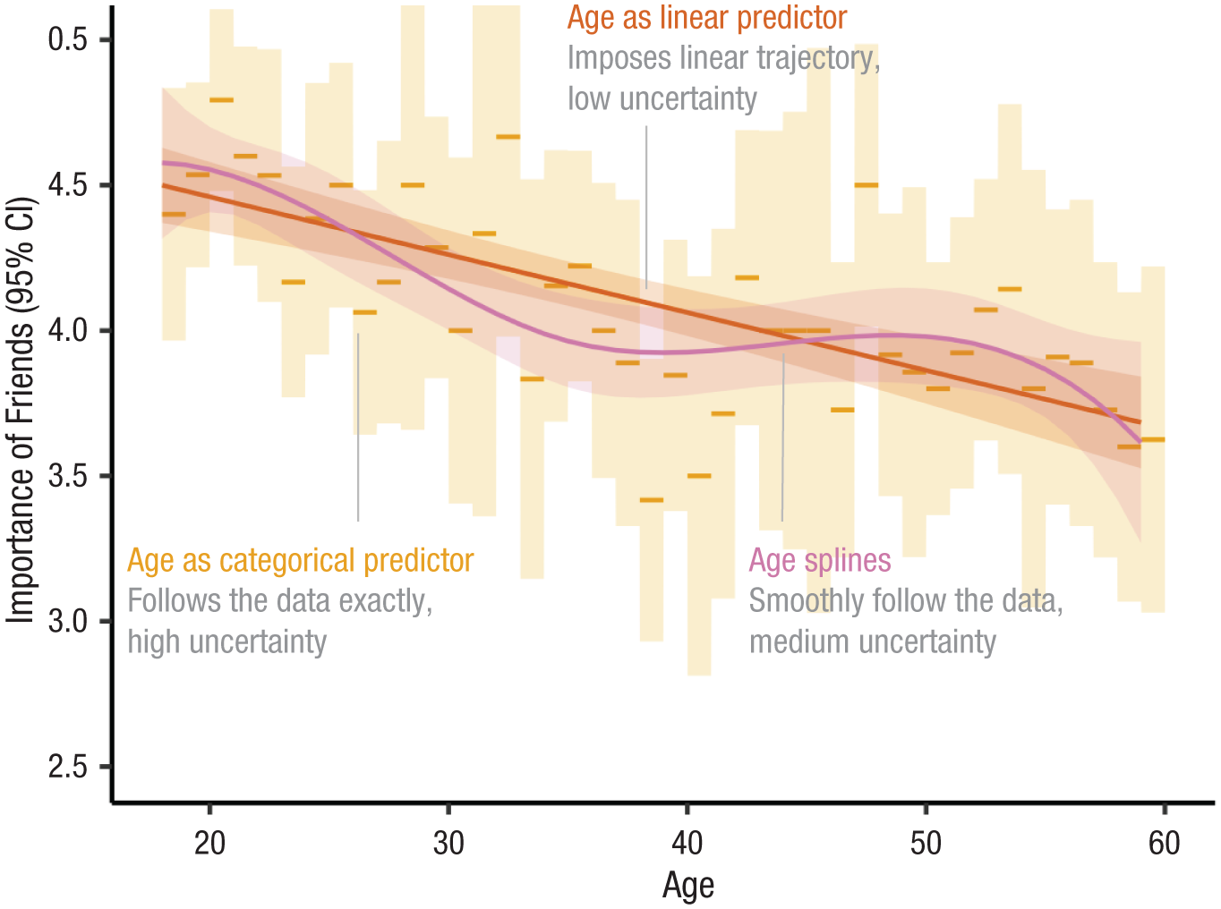
Respondents’ age varies from 18 to 59 years. How do we best include this variable in our analysis? If we simply include it as a linear predictor, we assume that friendship_importance changes with age in a linear manner (Fig. 4, orange-red line). If, instead, we include it as a categorical predictor (treating each year of age as its own category), we do not impose any assumptions about the functional form—but for some years, we have only few observations, resulting in a trajectory that jumps around a lot with wide confidence intervals (Fig. 4, light-orange line segments). So we may prefer a solution that lies somewhere between these two options.

Fig. 4.

Predicted importance of friends by age in three different simple linear models that include only age as a predictor, including age as a linear predictor or age as a categorical predictor or age splines (basis splines with 4 df). Shaded areas represent the respective 95% confidence intervals.

Contenders may be using coarser age categories (e.g., by creating 5- or 10-year bins) or using polynomials (e.g., including age² and maybe even age³; for arguments in favor of polynomials, see Kroc & Olvera Astivia, 2025). A third alternative is to use splines. These result in flexible, locally smooth trajectories. Unlike polynomials, splines enforce no global functional forms; unlike age categories, splines do not result in abrupt jumps in the trajectory. Both features may be desirable in many contexts, but splines are rarely used in psychological research—likely because they produce confusing regression outputs because they are implemented with the help of multiple synthetic variables that will each show up in the regression output with their own coefficients. Our goal in this section is to illustrate the merits of a workflow that does not require one to interpret individual coefficients, which circumvents the interpretation challenges posed by flexible modeling strategies, such as splines. In our regression model, we thus include age with the help of basis splines with 4 df (Fig. 4, purple line). For a more extensive discussion of alternative approaches, see Lopez-Ayala et al. (2025).¹¹

Interactions

If our two control variables, age and gender, interact, one may reasonably worry that omitting their interaction leads to residual confounding that biases the estimates of our target quantity. In addition, researchers may need to account for the possibility that the strength of the association between the outcome (friendship_importance) and the focal predictor (partner) depends on gender and age. One common strategy to handle both concerns is to include two- or even three-way interactions in the model specification.

However, researchers in psychology often favor parsimony in their model specification, avoiding the inclusion of such interactions (Rimpler et al. 2025). This default position is understandable because studying subgroup heterogeneity using interactions requires much larger samples than studying main effects. Focusing on the former can thus produce underpowered estimates that fail to replicate (e.g., Sommet et al., 2023), and it could lead to overfitted models with undesirable behavior out of sample. Moreover, opening the space of models that one considers increases researcher degrees of freedom and can expose writers to (sometimes unfair) charges of cherry-picking. Nevertheless, interactions remain an important part of the researcher’s toolbox because they help one relax strong assumptions about homogeneity of effects, capture key characteristics of the data-generating process, and limit residual confounding.

Researchers who choose to include interactions in their model face pragmatic concerns about interpretability. First, coefficients get harder to interpret as more parts are added to the model, and second, both researchers and readers may get distracted by individual coefficients, such as a significant three-way interaction that may simply reflect overfitting. Neither concern is much of an obstacle in the “models as prediction machines” workflow. First, we are not going to interpret (complex and confusing) raw coefficients directly but will instead use postestimation transformations to convert those coefficients into simple quantities with straightforward interpretation. The kind of transformations we propose are model-agnostic and make it easy to interpret the results of parsimonious or complex models alike. Second, although it is true that the coefficients associated with interaction terms can sometimes be data artifacts estimated with low precision, we recommend that researchers avoid interpreting these coefficients directly to focus on the target quantities that actually answer their research questions.

To illustrate this, our example includes all two-way interactions between the predictors. On the article’s accompanying website (https://j-rohrer.github.io/marginal-psych/), we push this even further and also include the three-way interaction to illustrate that this does not complicate model interpretation; the same function call is used to generate the target quantity. Furthermore, in this example, the inclusion of the interactions does not affect the precision with which the target quantity is estimated. This highlights how imprecision in the model coefficients does not automatically translate into imprecision in target quantities.

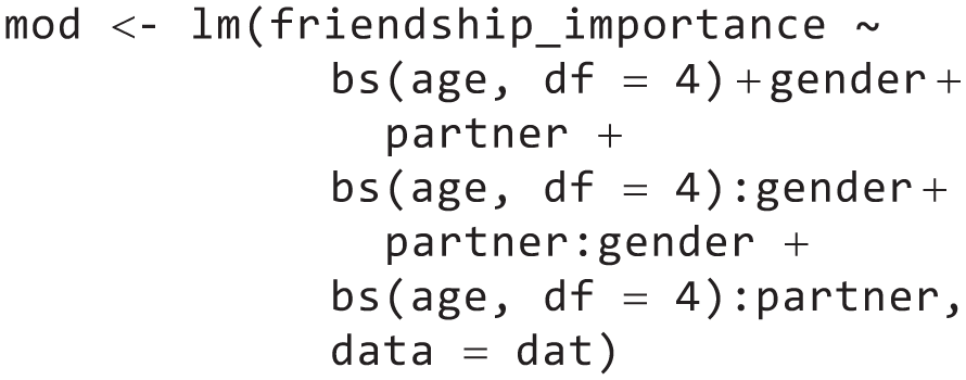
A linear regression model with splines and interactions

The foregoing discussion leads us to this regression model, which we can fit after loading the base R package splines :

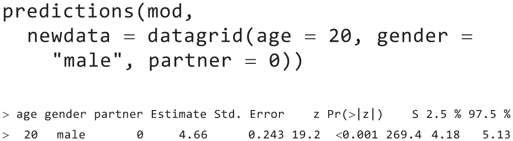
Now, we can use the model to calculate various target quantities. For example, we could predict friendship_importance for a 20-year-old man who reports no partner:

which tells us that our model expects a friendship_importance of 4.66, 95% confidence interval = [4.18, 5.13], for such an individual.

For the very same hypothetical man, we could also calculate the slope with respect to age:

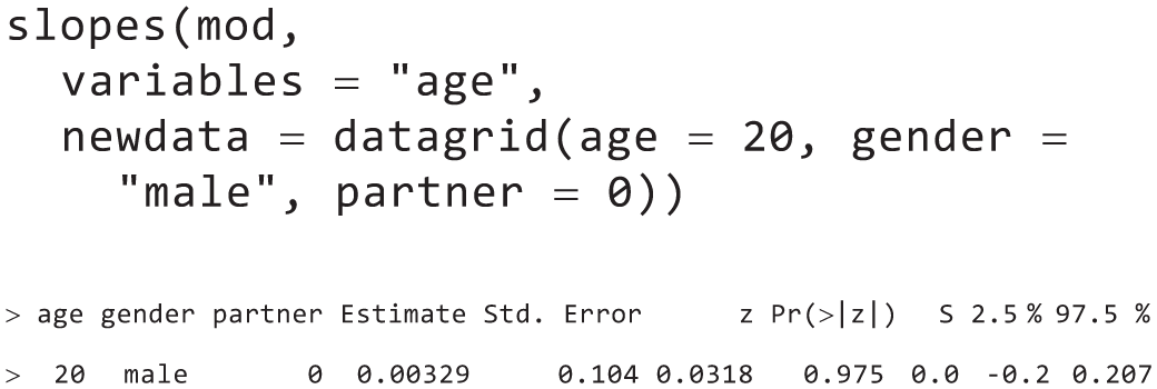
which tells us that for an individual with these characteristics, the model implies that friendship_importance changes by 0.003 points per year of age—that is, not much at all. The slope is also clearly not statistically significant, p = .975.

To calculate target quantities for every observation in the data, we simply omit the newdata argument:

which returns a table that contains the predictions for every single individual in the data and confidence intervals based on their observed predictor values (table omitted to save space).

Now, recall that the research question was whether people in romantic relationships, on average, assign less importance to their friends than people of the same age and gender who are not in romantic relationships. What is relevant for this are counterfactual comparisons, which we calculate for every individual in the data and then average:

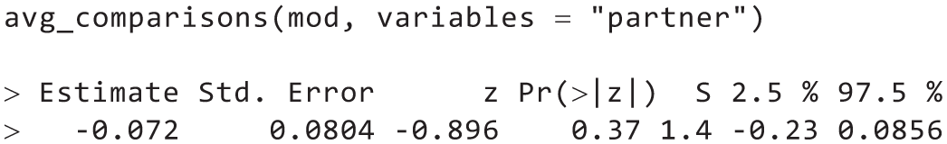
The answer is that on average and holding the other variables in our model constant, being in a romantic relationship is associated with 0.07 points lower friendship_importance (approximately 0.082 of the residual standard deviation). However, we find that this estimate is not significantly different from zero (p = .37).¹²

An ordinal regression model with splines and interactions

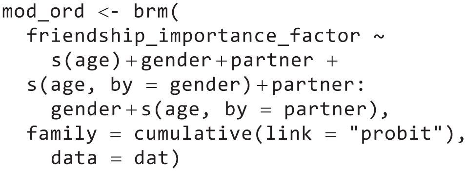
So far, we have simply conducted linear regressions, but that may be considered suspect given the nature of the outcome: a 5-point ordinal-response scale ranging from not important at all to very important. And in fact, barely anybody used the lower response options, and more than 40% picked the highest response option. This results in a distribution for which the assumptions of linear regression may be considered unrealistic.

We run an ordinal regression to see whether conclusions change. Here, we fit a cumulative ordinal model with a probit link using the brms package (Bürkner, 2018).¹³ In essence, this approach assumes a continuous, normally distributed standardized latent variable (“true” friendship_importance), which is translated into the ordinal response variable using thresholds that are estimated from the data. For example, people who score −3 or less on the standardized latent variable may report that their friends are not important at all, people who score more than that but below −2.7 may pick the second lowest response option, and so on (for a proper introduction to these models, see Bürkner & Vuorre, 2019). brms supports smoothing splines, which do not require us to predetermine the degrees of freedom (see Note 11), and so we implemented them here as well, resulting in the following model specification:

We can evaluate the association of interest using the same average comparison as before:

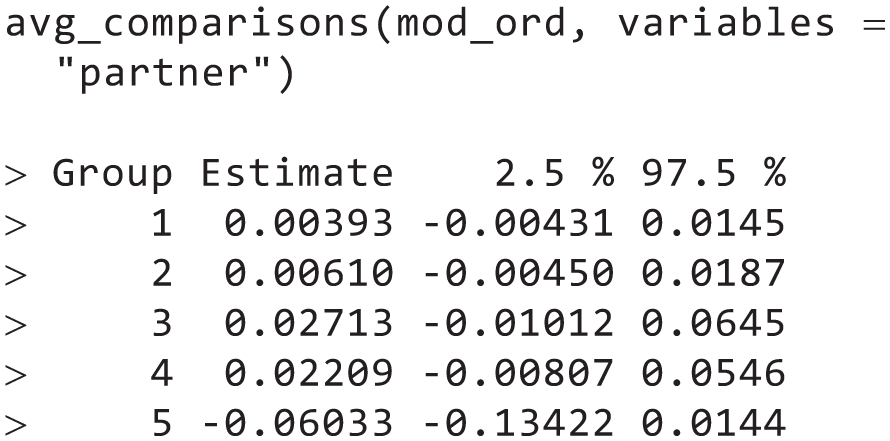
The resulting output, in this case, differs. By default, the output shows how the probability of any response category of friendship_importance changes when partner changes from 0 to 1. The response categories 1 to 4 become slightly more likely with partner = 1, and the probability of giving the highest rating, 5, decreases by 6 percentage points.¹⁴

We can also compute the comparison on the assumed underlying latent variable, which is the scale on which the model coefficients are reported in the regression output:

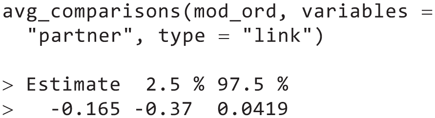
Here, results show that being in a romantic relationship is associated with 0.17 lower latent friendship importance. The latent variable is estimated as a standardized variable, which means that we can interpret this as a standardized effect-size metric. Thus, looking at the point estimates, the difference appears slightly stronger than in the linear model (−0.17 SD vs. −0.082 SD), but the 95% credible interval covers zero, meaning that once again, we probably should not rule out that there is no difference in the population.

Thus, treating the outcome as ordinal gives us slightly more detailed results because we can see how precisely the response shift between categories, but it does not affect our central conclusions: Although the point estimate suggests that people in a relationship report that their friends are slightly less important, the credible interval suggests that there is low certainty about the strength of the association, and it may also plausibly be zero or even negative.

Example 2: friends by chance

Everyday experience—and previous research—suggests that being spatially close to others can result in friendships. But does proximity also lead to friendships for people who are quite different from each other? We reanalyze data from a large field experiment conducted in third- to eighth-grade classrooms in rural Hungary previously reported in Rohrer et al. (2021).¹⁵ Proximity was experimentally manipulated by randomizing each classroom’s seating chart at the beginning of the school semester; thus, students randomly ended up next to each other (deskmate = 1) or not (deskmate = 0). At the end of the semester, students listed up to five best friends from their classroom, which allows us to determine which pairs of students had formed friendships (friendship = 1). In addition, we know students’ gender and grade point average (GPA) before the experiment, which allows us to investigate whether proximity also “works” for girls seated next to boys (who are quite unlikely to befriend each other at that age) or students with discrepant levels of academic achievement.

A Bayesian generalized multimembership mixed-effects model

The data we analyze have a nested structure: students, in pairs, in classrooms. To account for this, we fit a flexible Bayesian multilevel model using the brms package. Once again, our goal is not to defend one particular model specification but rather to show that interpretation can proceed easily even if the model we fit is complex. Our intent is to show that even if readers are unfamiliar with Bayesian analysis or multilevel models, they can still understand our workflow and the results it produces.

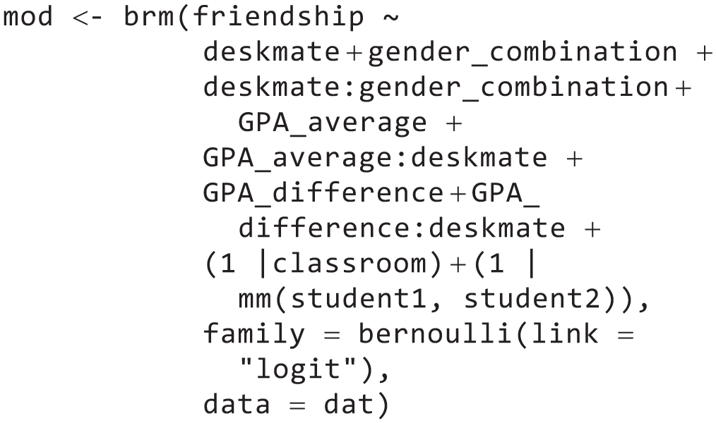
The unit of observation in this analysis is pairs of students that are nested within classrooms. For each pair, we know (a) whether they are deskmates, (b) their gender_combination (either both boys, or one girl and one boy, or both girls), (c) their GPA_average (i.e., the average GPA across both students) and their absolute GPA_difference (i.e., the GPA discrepancy between both students), and (d) whether they report a friendship at the end of the study. We end up with the following binary logistic multilevel model:

Note that we have included two different types of random intercepts: classroom intercepts, (1 |classroom), to account for nesting within classrooms, and student intercepts, mm(1|student1, student2), to account for the fact that the same student is part of multiple pairs.¹⁶

Average effects on different scales

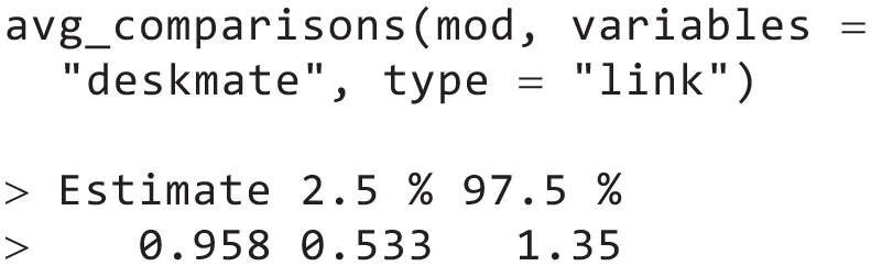
In principle, we could evaluate this model on the log-odds scale on which the coefficients are estimated. For example, the coefficient of deskmate is b = 0.19. Given all interactions in the model, this coefficient will be sensitive to coding decisions, so instead, we calculate the average effect on the log-odds scale:

This gives us an average effect of 0.958 on the log-odds of friendship (95% credible interval = [0.53, 1.35]). Unfortunately, log-odds of friendship are not a particularly intuitive unit, so we may want to switch to the scale of the outcome (friendships)—which is the default behavior of marginaleffects .

First, we look at the average (counterfactual) prediction if all pairs were (or were not) deskmates:

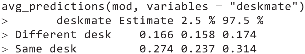
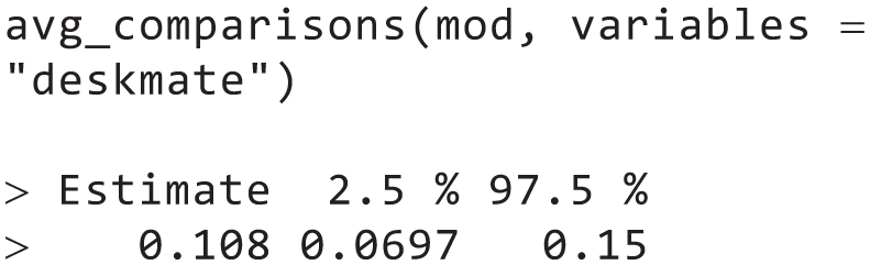
This tells us that the model predicts an average friendship probability of 27.4% for deskmates and 16.6% for nondeskmates. Then, we calculate the ATE, which is the difference between these two numbers:

We find that being seated next to each other increases the probability of a friendship by 11 percentage points (95% credible interval = [0.07, 0.15]).

Comparing the effect with the fast-friends procedure

Are the estimated effects we reported above large? To answer this question, it may be useful to compare our estimates with the effects of other interventions meant to foster friendships. For example, one staple of psychological research is the fast-friends procedure (Aron et al., 1997; Page-Gould et al., 2008), in which two participants are paired up and take turns answering questions that escalate in the degree of self-disclosure involved, from mild (“Would you like to be famous? In what way?”) to severe (“When did you last cry in front of another person?”). Echols and Ivanich (2021) implemented such a procedure in U.S. middle school students and found that participants who underwent the intervention in three sessions over 3 months were 10 percentage points more likely to become friends. This seems very close to the 11 percentage point effect we observed in our analysis. Would it be justified to conclude that the effects are practically the same?

In a frequentist framework, this would be a use case for an equivalence test, such as the two one-sample test, or TOST (Lakens et al., 2018). All the functions in the marginaleffects package have an equivalence argument that can execute a TOST for any of the quantities that the package estimates: predictions, comparisons, slopes, and even complex quantities derived for (non)linear hypothesis tests. Because the model that we estimated above is Bayesian, marginaleffects will not conduct a TOST by default. Instead, the equivalence argument will quantify the size of the posterior density in a region of practical equivalence (ROPE; Kruschke, 2018; Makowski et al., 2019).

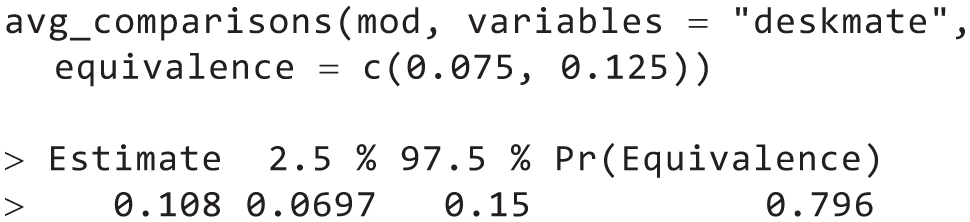
To do this, we first need to define a range around the estimated effect size of the fast-friends procedure. This range must be based on substantive and application-specific considerations. For instance, the analyst could decide that if the effect of deskmates falls within ± a quarter of the fast-friends effect, they will be considered “equivalent” to each other. In that case, the analyst would specify a ROPE of [0.075, 0.125]. Now, we can use the equivalence argument to calculate how likely it is that the effect of sitting next to each other falls into this ROPE:

This suggests that based on our model, priors, and data, there is an 80% chance that the effect of sitting next to each other is practically equivalent to the previously reported effect of the fast-friends procedure.¹⁷

Moderation by similarity

Having looked at the average effect of the intervention, we still do not yet know whether being seated next to each other also works for dissimilar students. Here, in line with best-practice recommendations, we keep evaluating effects on the response scale (Mize, 2019).

First, we can separately calculate average effects depending on gender_combination:

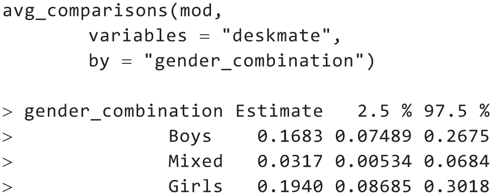
We find that the average effects are quite large for pairs of boys (b₁ = 17 percentage points, 95% credible interval = [0.07, 0.27]) and pairs of girls (b₃ = 19 percentage points, 95% credible interval = [0.09, 0.30]) but much smaller for pairs of boys and girls (b₂ = 3 percentage points, 95% credible interval = [0.01, 0.07]). Thus, although proximity does seem to work for gender-mixed pairs, the estimated effect is very small in absolute terms. We can easily compare all three average effects with each other in pairwise manner:

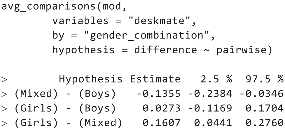
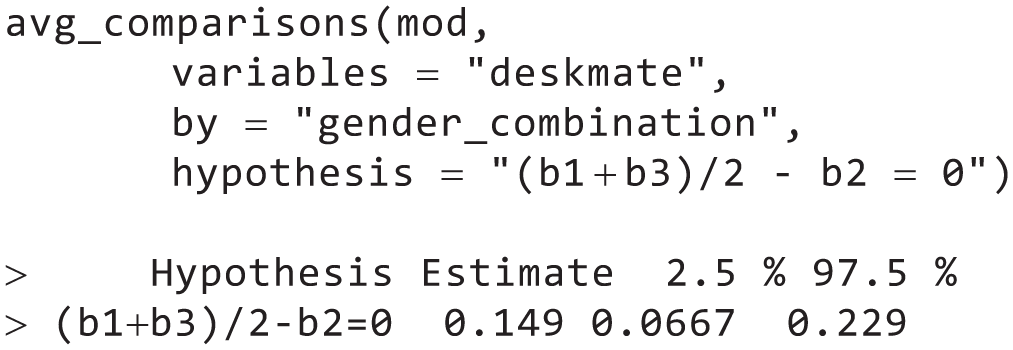
For example, the average effect of deskmate is 0.03 larger in pairs of girls than in pairs of boys (95% credible interval = [−0.12, 0.17]). We may also want to compare gender-matched dyads (pairs of girls, pairs of boys) with gender-mismatched dyads (pairs of a girl and a boy): (b_{Two girls} + b_{Two boys}) / 2 = b_{One girl one boy}, which can also be written as (b_{Two girls} + b_{Two boys}) / 2 − b_{One girl one boy} = 0. This can be achieved by using a different hypothesis argument, with the letter “b” followed by a number that indicates the row number in which the original estimates appeared:

This reveals that among gender-matched dyads, the effect of deskmate is 15 percentage points larger than among gender-mismatched dyads (95% credible interval = [0.07, 0.23]). Thus, the intervention appears to create a lot more friendships among gender-matched dyads.

Note that the types of questions we asked in this section—about effect moderation—are the same as the questions that typically interest researchers who interpret the interaction coefficients of their regression models. But instead of framing the hypothesis in terms of abstract quantities, such as the size of a “two-way interaction term,” we encourage analysts to recast it more explicitly in terms of the variables and quantities that actually interest them: “Is the effect of deskmates larger for matched pairs or mixed pairs?” When framed in this way, the research question is easier for readers to understand, and it maps clearly onto quantities that are easy to compute with marginaleffects.

Causal moderation and all-else-equal claims

In the previous section, we used the avg_comparisons() function and its by argument to compute the average effect of deskmate within each subgroup of gender_combinations. Under the hood, marginaleffects started by computing unit-level estimates in the full data set and then aggregated those estimates within each level of the moderator variable. This approach makes sense if our goal is simply to establish whether the effect (or association) is stronger in some subsets of the population. Indeed, our analysis showed that the positive effect of deskmate on the probability of striking a friendship was much stronger in matched-gender pairs than in mixed-gender pairs. Unfortunately, the estimates reported above cannot tell us why the effects differ between subgroups. They cannot establish that the effect changes because of the moderator because the strata defined by the moderator may also vary in other variables that could explain the difference in effects.

Researchers often do have the more ambitious research goal of establishing that some moderator causally affects the effect of interest.¹⁸ In that context, researchers must pay special attention to the distribution of potential confounders in the various moderator strata. If such confounders of the moderation exist, it is important to conduct a counterfactual analysis that holds their distribution constant across moderator strata.

On the website that accompanies this article (https://j-rohrer.github.io/marginal-psych/), we illustrate how to conduct this type of causal moderation analysis in marginaleffects , investigating whether GPA_difference potentially causally changes the effects of deskmate, holding constant the distribution of gender_combination (a plausible confounder because gender affects GPA and thus gender-mismatched pairs will differ more strongly in GPA) across levels of the moderator. For pairs of students with a small GPA_difference (−1 SD), our model implies a somewhat larger effect (0.14, 95% credible interval = [0.06, 0.18]) than for pairs of students with a large GPA_difference (+1 SD; 0.10, 95% credible interval = [0.04, 0.16]). But the difference is quite small and estimated with a lot of uncertainty, 0.02, 95% credible interval = [−0.07, 0.12], so that we cannot conclude anything.

Discussion

Researchers routinely interpret regression coefficients to make sense of their statistical models. Our starting point was that such coefficients can often be confusing, and we presented an alternative framework that treats statistical models as counterfactual prediction machines that can be queried in a targeted manner to answer one’s research questions. We then showed how to implement such analyses with the help of marginaleffects .

As mentioned earlier, this package for R and Python covers a lot more that what we could show here, including support for machine-learning models, inverse probability weighting, matching, and multiple imputation for missing data. Up-to-date information and dozens of tutorials are freely available on the package website (https://marginaleffects.com/). However, note that it does not cover structural equation models, which limits possibilities with respect to latent-variable models. If latent-variable modeling is a central concern, analysts may consider using lavaan (Rosseel et al., 2025) and the EffectLiteR companion package (Mayer et al., 2016).

Room for mistakes

We claimed that the interpretation of regression coefficients is error prone. But is the approach we suggest here really less error prone? In both the standard and prediction-machines workflows, researchers need to select, specify, and fit a statistical or machine-learning model. This means that in both approaches, they need to pay close attention to issues such as omitted variables, “bad controls” (Cinelli et al., 2024), and appropriate functional forms. Moreover, concerns such as statistical power apply under both frameworks.¹⁹

When regression coefficients are interpreted, one source of error is whether the coefficients really address the research question of interest. In our marginaleffects framework, the corresponding source of error is whether the specified target quantity really addresses the research question of interest. We believe that thinking in terms of target quantities may ultimately be more intuitive and thus easier to master, although it is, of course, an empirical question whether researchers will make fewer mistakes. For those researchers who are not entirely sure which research question they want to address and who start with an imprecise verbalization (“What’s the role of X for Y?”), the need to actually spell out target quantities rather than just looking at the regression coefficients enforces more clarity. This also applies to researchers who start with a “coefficient-oriented” question, such as “What’s the magnitude of the interaction between X and Z?” or “Which interaction is larger, X and Z or X and W?” As illustrated in our second worked example, substantively, a statistical interaction may translate into subgroup comparisons of counterfactual comparisons, or counterfactual comparisons of counterfactual comparisons. Beyond this, conclusions may hinge on which levels of the purported moderator are compared. Although the requirement for more specificity may appear like a nuisance, we believe that it is worthwhile to move from research questions in terms of abstract statistical quantities to more substantively focused research questions about specific comparisons.

A more minor source of error that can be eliminated with the help of our framework is coding decisions meant to render coefficients more interpretable (e.g., different coding schemes for categorical variables, centering continuous variables), which result in models that make equivalent predictions. Because coefficients need not be interpretable in the first place, these decisions become irrelevant.²⁰

The future of statistics teaching

It is one question whether researchers trained to interpret regression coefficients profit from adding a framework that focuses on target quantities; another one is which approach should be taught. When focusing on target quantities, some parts of the curriculum remain unchanged—students still need to understand how to set up a model, how to quantify and interpret uncertainty, and how to navigate the trade-off between model flexibility and overfitting risk. Other parts can be radically simplified, such as instructions for how to make sense of interaction coefficients or various coding schemes for categorical variables.

The abstraction to think of statistical models as predictions machines may also make it easier to teach more advanced models in an accessible manner, such as binary logistic regression (which is already routinely included in curricula) or ordinal models (which have not experienced much uptake despite multiple attempts to popularize them; Bürkner & Vuorre, 2019; Liddell & Kruschke, 2018). Finally, a model-agnostic framework to interpretation prepares students for machine-learning methods that are clearly growing more popular in psychology and other fields (for a worked example, see Arel-Bundock, 2026, Chapter 13).

Any time that may be saved could be used to focus on the more substantive aspects of statistical modeling, such as how one can spell out clear estimands and which identification assumptions are necessary so that the model actually returns the correct answer (Lundberg et al., 2021). We believe that researchers are currently undertrained in these domains. This is illustrated by the fact that often, scientific arguments hinge on uncertainty about what researchers are trying to estimate in the first place. Is the marshmallow test meant to correlate with achievement, predict achievement beyond certain covariates, or measure some trait that causally affects achievement (Doebel et al., 2020; Falk et al., 2020; Watts & Duncan, 2020; Watts et al., 2018)? What is the estimand underlying the question whether there is a midlife crisis (Kratz & Brüderl, 2025)? And the issue of unclear estimands has also surfaced in the metascientific discussions about the value of many-analysts projects (Auspurg & Brüderl, 2021; Rohrer et al., 2025) and multiverse analyses (Auspurg, 2025; Auspurg & Brüderl, 2024).

Dealing with researcher degrees of freedom

One risk to consider is that the approach we champion results in more flexibility in model interpretation—a model containing only a handful of coefficients may result in dozens of possible target quantities. This increase in researcher degrees of freedom could be abused, with researchers strategically reporting the target quantities that “work” for their narrative purposes, resulting in a biased literature. This risk may be aggravated when reviewers do not have a firm grasp on how to connect research questions to statistical analyses so that any target quantity appears defensible to them. To combat this issue, we recommend that researchers rely on established measures to deal with researcher degrees of freedom and additionally take into account target quantities. For example, if researchers preregister a regression model, they should additionally preregister the primary target quantity they are going to calculate and interpret. Some existing preregistration templates already require authors to spell out how model results will be interpreted; actually spelling out target quantities adds more precision to this step.

Researchers may also conduct robustness analyses to probe whether a different choice of target quantity would result in different conclusions. At this point, it is important to keep in mind that different target quantities based on the same model are responses to different research questions returned by the same model. Because they answer different research questions, they should not simply be (implicitly or explicitly) aggregated because this would amount to averaging apples and oranges. And because they are returned by the same model, they are fully compatible with each other even if on first glance, they may appear contradictory.

To illustrate such ostensible contradictions, consider the study underlying our second example, in which students were randomly seated next to each other (Rohrer et al., 2021). Considering the central research question of whether the effectiveness of the intervention varies depending on the similarity of the students, results appear different depending on the scale on which they are evaluated. On the link scale, there is no effect modification—which is reflected by the fact that the coefficient of the interaction is not significantly different from zero. But on the response scale, there is clear effect modification—the probability of a friendship increased a lot more when similar (rather than dissimilar) students were placed next to each other.

If in such a situation findings are presented on only one scale, the choice of scale will most likely determine whether readers conclude that there is an interaction. Pragmatically speaking, there may be arguments for both scales—the link scale is what psychologists are used to (and may be deemed more relevant for basic research questions, Simonsohn, 2017), and the response scale is recommended by modern guidelines (Ai & Norton, 2003; McCabe et al., 2022; Mize, 2019). In such a situation, reporting results on both scales—and thus multiple target quantities—is a straightforward way to increase transparency.

Model mechanics and the needs of applied researchers

Another risk to consider is that the approach results in a loss of understanding of model mechanics; after all, we touted as a benefit that treating models as prediction machines removes the need to fully understand how the coefficients make the machine go. But sometimes it may still be necessary to “look under the hood” to figure out what went wrong. Here, we suggest that a greater division of cognitive labor may be desirable, with expert statisticians focusing on model mechanics and applied researchers operating on a higher level of abstraction, focusing on articulating clear research questions and using their substantive knowledge to assess the plausibility of the assumptions necessary to answer them. Of course, there already is a community of expert statisticians, but at the current point, applied researchers are to some extent expected to immerse themselves in the nitty-gritty details of statistical modeling. These applied researchers, we hope, will profit from a framework that allows them to focus on substantively meaningful target quantities over at times confusing coefficients.

To conclude, we have shown that treating models as prediction machines and centering analysis on clearly defined target quantities can turn confusing coefficients into transparent answers to meaningful, substantive questions. The workflow we introduced is convenient because it is model-agnostic; it works the same across linear, generalized, multilevel, ordinal, Bayesian, and machine-learning models. This means that researchers can fit flexible specifications without sacrificing interpretability. Our workflow also reduces cognitive load, curbs common mistakes, and allows analysts and readers to maintain focus on what really matters: theories, questions, estimands, assumptions, and tests.

Footnotes

Acknowledgements

We thank Mattan S. Ben-Shachar, Jamie Cummins, Saloni Dattani, Ron Garcia, A. Solomon Kurz, Daniel Lüdecke, Stefan Schmukle, Federico Vaggi, Aki Vehtari, and Aleš Vomácˇka for helpful comments. The publication of this article was supported by the Open Access Publishing Fund of Leipzig University. This article was made available as a preprint on PsyArXiv: https://osf.io/preprints/psyarxiv/g4s2a_v2. All data and analysis code to reproduce the worked examples are made available on the website https://j-rohrer.github.io/marginal-psych/. And an archived snapshot of the repository is preserved on Zenodo, .

Transparency

Action Editor: Rogier Kievit

Editor: David A. Sbarra

Author Contributions

Julia M. Rohrer: Conceptualization; Investigation; Methodology; Visualization; Writing – original draft; Writing – review & editing.

Vincent Arel-Bundock: Conceptualization; Investigation; Methodology; Software; Writing – original draft; Writing – review & editing.

ORCID iD

Julia M. Rohrer

Notes

References

Norton

E. C.

(2003). Interaction terms in logit and probit models. Economics Letters, 80(1), 123–129. https://doi.org/10.1016/S0165-1765(03)00032-6

Arel-Bundock

(2026). Model to meaning: How to interpret statistical models with R and Python. Chapman and Hall/CRC.

Arel-Bundock

Greifer

Heiss

(2024). How to interpret statistical models using marginaleffects for R and Python. Journal of Statistical Software, 111(9), 1–32. https://doi.org/10.18637/jss.v111.i09

Aron

Melinat

Aron

E. N.

Vallone

R. D.

Bator

R. J.

(1997). The experimental generation of interpersonal closeness: A procedure and some preliminary findings. Personality & Social Psychology Bulletin, 23(4), 363–377. https://doi.org/10.1177/0146167297234003

Auspurg

(2025). Robustness is better assessed with a few thoughtful models than with billions of regressions. Proceedings of the National Academy of Sciences of the United States of America, 122(43), Article e2521917122. https://doi.org/10.1073/pnas.2521917122

Auspurg

Brüderl

(2021). Has the credibility of the social sciences been credibly destroyed? Reanalyzing the “many analysts, one data set” project. Socius, 7. https://doi.org/10.1177/23780231211024421

Auspurg

Brüderl

(2024). Toward a more credible assessment of the credibility of science by many-analyst studies. Proceedings of the National Academy of Sciences of the United States of America, 121(38), Article e2404035121. https://doi.org/10.1073/pnas.2404035121

Bansak

(2021). Estimating causal moderation effects with randomized treatments and non-randomized moderators. Journal of the Royal Statistical Society Series A: Statistics in Society, 184(1), 65–86. https://doi.org/10.1111/rssa.12614

Bürkner

P.-C.

(2018). Advanced Bayesian multilevel modeling with the R package brms. The R Journal, 10(1), 395–411. https://doi.org/10.32614/RJ-2018-017

10.

Bürkner

P.-C.

Vuorre

(2019). Ordinal regression models in psychology: A tutorial. Advances in Methods and Practices in Psychological Science, 2(1), 77–101. https://doi.org/10.1177/2515245918823199

11.

Burnham

K. P.

Anderson

D. R.

(Eds.). (2002). Model selection and multimodel inference: A practical information-theoretic approach (2nd ed.). Springer. https://doi.org/10.1007/b97636

12.

Chatton

Rohrer

J. M.

(2024). The causal cookbook: Recipes for propensity scores, G-computation, and doubly robust standardization. Advances in Methods and Practices in Psychological Science, 7(1). https://doi.org/10.1177/25152459241236149

13.

Cinelli

Forney

Pearl

(2024). A crash course in good and bad controls. Sociological Methods & Research, 53(3), 1071–1104. https://doi.org/10.1177/00491241221099552

14.

Davies

H. T.

Crombie

I. K.

Tavakoli

(1998). When can odds ratios mislead? BMJ, 316(7136), 989–991. https://doi.org/10.1136/bmj.316.7136.989

15.

Doebel

Michaelson

L. E.

Munakata

(2020). Good things come to those who wait: Delaying gratification likely does matter for later achievement (a commentary on Watts, Duncan, & Quan, 2018). Psychological Science, 31(1), 97–99. https://doi.org/10.1177/0956797619839045

16.

Echols

Ivanich

(2021). From “Fast Friends” to true friends: Can a contact intervention promote friendships in middle school? Journal of Research on Adolescence, 31(4), 1152–1171. https://doi.org/10.1111/jora.12622

17.

Esterling

K. M.

Brady

Schwitzgebel

(2025). The necessity of construct and external validity for deductive causal inference. Journal of Causal Inference, 13(1), Article 20240002. https://doi.org/10.1515/jci-2024-0002

18.

Falk

Kosse

Pinger

(2020). Re-revisiting the marshmallow test: A direct comparison of studies by Shoda, Mischel, and Peake (1990) and Watts, Duncan, and Quan (2018). Psychological Science, 31(1), 100–104. https://doi.org/10.1177/0956797619861720

19.

Greifer

Worthington

Iacus

King

(2025). Clarify: Simulation-based inference for regression models. The R Journal, 16(2), 154–174. https://doi.org/10.32614/rj-2024-015

20.

Halvorson

M. A.

McCabe

C. J.

Kim

D. S.

Cao

King

K. M.

(2022). Making sense of some odd ratios: A tutorial and improvements to present practices in reporting and visualizing quantities of interest for binary and count outcome models. Psychology of Addictive Behaviors, 36(3), 284–295. https://doi.org/10.1037/adb0000669

21.

Hayes

A. F.

Glynn

C. J.

Huge

M. E.

(2012). Cautions regarding the interpretation of regression coefficients and hypothesis tests in linear models with interactions. Communication Methods and Measures, 6(1), 1–11. https://doi.org/10.1080/19312458.2012.651415

22.

Keele

Stevenson

R. T.

Elwert

(2020). The causal interpretation of estimated associations in regression models. Political Science Research and Methods, 8(1), 1–13. https://doi.org/10.1017/psrm.2019.31

23.

Kratz

Brüderl

(2025). Assessing age trajectories (of subjective well-being): Clarifying estimands, identification assumptions, and estimation strategies. European Sociological Review. Advance online publication. https://doi.org/10.1093/esr/jcaf038

24.

Kroc

Olvera Astivia

O. L.

(2025). The case for the curve: Parametric regression with second- and third-order polynomial functions of predictors should be routine. Psychological Methods, 30(6), 1277–1293. https://doi.org/10.1037/met0000629

25.

Kruschke

J. K.

(2018). Rejecting or accepting parameter values in Bayesian estimation. Advances in Methods and Practices in Psychological Science, 1(2), 270–280. https://doi.org/10.1177/2515245918771304

26.

Lakens

Scheel

A. M.

Isager

P. M.

(2018). Equivalence testing for psychological research: A tutorial. Advances in Methods and Practices in Psychological Science, 1(2), 259–269. https://doi.org/10.1177/2515245918770963

27.

Liddell

T. M.

Kruschke

J. K.

(2018). Analyzing ordinal data with metric models: What could possibly go wrong? Journal of Experimental Social Psychology, 79, 328–348. https://doi.org/10.1016/j.jesp.2018.08.009

28.

Liebig

Goebel

Schröder

Grabka

Richter

Schupp

Bartels

Fedorets

Franken

Jacobsen

Kara

Krause

Kröger

Metzing

Nebelin

Schacht

Schmelzer

Schmitt

Schnitzlein

, . . . Deutsches Institut für Wirtschaftsforschung (DIW Berlin). (2022). SOEP-Übungsdatensatz, Daten der Jahre 2015-2019 [SOEP practice data set] [Data set]. SOEP Socio-Economic Panel Study. https://doi.org/10.5684/SOEP.PRACTICE.V36

29.

Lopez-Ayala

Riley

R. D.

Collins

G. S.

Zimmermann

(2025). Dealing with continuous variables and modelling non-linear associations in healthcare data: practical guide. The BMJ, 390, Article e082440. https://doi.org/10.1136/bmj-2024-082440

30.

Lundberg

Johnson

Stewart

B. M.

(2021). What is your estimand? Defining the target quantity connects statistical evidence to theory. American Sociological Review, 86(3), 532–565. https://doi.org/10.1177/00031224211004187

31.

Makowski

Ben-Shachar

M. S.

Chen

S. H. A.

Lüdecke

(2019). Indices of effect existence and significance in the Bayesian framework. Frontiers in Psychology, 10, Article 2767. https://doi.org/10.3389/fpsyg.2019.02767

32.

Mayer

Dietzfelbinger

Rosseel

Steyer

(2016). The EffectLiteR approach for analyzing average and conditional effects. Multivariate Behavioral Research, 51(2–3), 374–391. https://doi.org/10.1080/00273171.2016.1151334

33.

McCabe

C. J.

Halvorson

M. A.

King

K. M.

Cao

Kim

D. S.

(2022). Interpreting interaction effects in generalized linear models of nonlinear probabilities and counts. Multivariate Behavioral Research, 57(2–3), 243–263. https://doi.org/10.1080/00273171.2020.1868966

34.

McNeish

(2023). A practical guide to selecting and blending approaches for clustered data: Clustered errors, multilevel models, and fixed-effect models. Psychological Methods. Advance online publication. https://doi.org/10.1037/met0000620

35.

Mize

(2019). Best practices for estimating, interpreting, and presenting nonlinear interaction effects. Sociological Science, 6, 81–117. https://doi.org/10.15195/v6.a4

36.

Molnar

(2020). Interpretable machine learning. Lulu.com. https://www.academia.edu/download/103712558/Christoph_Molnar_Interpretable_Machine_Learning_lulu.com_20210426_.pdf

37.

Nickerson

R. S.

(2004). Cognition and chance: The psychology of probabilistic reasoning. Psychology Press. https://doi.org/10.4324/9781410610836

38.

Norton

E. C.

Dowd

B. E.

Garrido

M. M.

Maciejewski

M. L.

(2024). Requiem for odds ratios. Health Services Research, 59(4), Article e14337. https://doi.org/10.1111/1475-6773.14337

39.

Page-Gould

Mendoza-Denton

Tropp

L. R.

(2008). With a little help from my cross-group friend: Reducing anxiety in intergroup contexts through cross-group friendship. Journal of Personality and Social Psychology, 95(5), 1080–1094. https://doi.org/10.1037/0022-3514.95.5.1080

40.

Rimpler

Kiers

H. A. L.

van Ravenzwaaij

(2025). To interact or not to interact: The pros and cons of including interactions in linear regression models. Behavior Research Methods, 57(3), 92. https://doi.org/10.3758/s13428-025-02613-6

41.

Rohrer

J. M.

(2018). Thinking clearly about correlations and causation: Graphical causal models for observational data. Advances in Methods and Practices in Psychological Science, 1(1), 27–42. https://doi.org/10.1177/2515245917745629

42.

Rohrer

J. M.

Arslan

R. C.

(2021). Precise answers to vague questions: Issues with interactions. Advances in Methods and Practices in Psychological Science, 4(2). https://doi.org/10.1177/25152459211007368

43.

Rohrer

J. M.

Hünermund

Arslan

R. C.

Elson

(2022). That’s a lot to process! Pitfalls of popular path models. Advances in Methods and Practices in Psychological Science, 5(2). https://doi.org/10.1177/25152459221095827

44.

Rohrer

J. M.

Keller

Elwert

(2021). Proximity can induce diverse friendships: A large randomized classroom experiment. PLOS ONE, 16(8), Article e0255097. https://doi.org/10.1371/journal.pone.0255097

45.

Rohrer

J. M.

Seifert

I. S.

Arslan

R. C.

Sun

Schmukle

S. C.

(2024). The effects of satisfaction with different domains of life on general life satisfaction vary between individuals (but we cannot tell you why). Collabra. Psychology, 10(1), Article 121238. https://doi.org/10.1525/collabra.121238

46.

Rohrer

J. M.

Smith

G. D.

Munafò

(2025). What can be learned when multiple analysts arrive at different estimates. European Journal of Epidemiology, 40(5), 493–495. https://doi.org/10.1007/s10654-025-01249-2

47.

Rosseel

Jorgensen

T. D.

De Wilde

(2025). lavaan: Latent variable analysis. https://doi.org/10.32614/CRAN.package.lavaan

48.

Ruppert

Wand

M. P.

Carroll

R. J.

(2003). Semiparametric regression. Cambridge series in statistical and probabilistic mathematics. Cambridge University Press.

49.

Simonsohn

(2017). [57] Interactions in logit regressions: Why positive may mean negative. Datacolada. http://datacolada.org/57

50.

Simonsohn

(2024). Interacting with curves: How to validly test and probe interactions in the real (nonlinear) world. Advances in Methods and Practices in Psychological Science, 7(1). https://doi.org/10.1177/25152459231207787

51.

Sommet

Weissman

D. L.

Cheutin

Elliot

A. J.

(2023). How many participants do I need to test an interaction? Conducting an appropriate power analysis and achieving sufficient power to detect an interaction. Advances in Methods and Practices in Psychological Science, 6(3). https://doi.org/10.1177/25152459231178728

52.

Sørensen

Ø.

Fjell

A. M.

Walhovd

K. B

. (2023). Longitudinal modeling of age-dependent latent traits with generalized additive latent and mixed models. Psychometrika, 88(2), 456–486. https://doi.org/10.1007/s11336-023-09910-z

53.

Sørensen

Ø.

McCormick

E. M

. (2025). Modeling cycles, trends and time-varying effects in dynamic structural equation models with regression splines. Multivariate Behavioral Research, 60(5), 1013–1028. https://doi.org/10.1080/00273171.2025.2507297

54.

StataCorp. (Ed.). (2025). Stata 19 user guide. Stata Press. https://www.stata.com/manuals/u.pdf

55.

Tomz

Wittenberg

King

(2003). Clarify: Software for interpreting and presenting statistical results. Journal of Statistical Software, 8, 1–30. https://doi.org/10.18637/JSS.V008.I01

56.

VanderWeele

T. J.

(2009). On the distinction between interaction and effect modification. Epidemiology, 20(6), 863–871. https://doi.org/10.1097/EDE.0b013e3181ba333c

57.

Watts

T. W.

Duncan

G. J.

(2020). Controlling, confounding, and construct clarity: Responding to criticisms of “revisiting the marshmallow test” by Doebel, Michaelson, and Munakata (2020) and Falk, Kosse, and Pinger (2020). Psychological Science, 31(1), 105–108. https://doi.org/10.1177/0956797619893606

58.

Watts

T. W.

Duncan

G. J.

Quan

(2018). Revisiting the marshmallow test: A conceptual replication investigating links between early delay of gratification and later outcomes. Psychological Science, 29(7), 1159–1177. https://doi.org/10.1177/0956797618761661

59.

Westreich

Greenland

(2013). The Table 2 fallacy: Presenting and interpreting confounder and modifier coefficients. American Journal of Epidemiology, 177(4), 292–298. https://doi.org/10.1093/aje/kws412

60.

Wickham

(2014). Tidy data. Journal of Statistical Software, 59(10), 1–23. https://doi.org/10.18637/jss.v059.i10

61.

Williams

(2012). Using the margins command to estimate and interpret adjusted predictions and marginal effects. The Stata Journal, 12(2), 308–331. https://doi.org/10.1177/1536867X1201200209

62.

Wood

S. N.

(2017). Generalized additive models: An introduction with R. Chapman and Hall/CRC. https://doi.org/10.1201/9781315370279

63.

Wysocki

A. C.

Lawson

K. M.

Rhemtulla

(2022). Statistical control requires causal justification. Advances in Methods and Practices in Psychological Science, 5(2). https://doi.org/10.1177/25152459221095823

Models as Prediction Machines: How to Convert Confusing Coefficients Into Clear Quantities

Abstract

Keywords

Coefficients Can Confuse

Interactions

Nonlinearity in the predictors

Nonlinear link functions

Categorical predictors

The Table 2 fallacy

Models as Prediction Machines

Workflow: Targets, Tests, and Tools

Target quantities

Predictions

Comparisons

Slopes

Individuals, averages, and target populations

Quantification on different scales

Tests

Tools

Worked Examples

Example 1: relationship status and the importance of friends

Controlling for confounders in a flexible manner

Splines

Interactions

A linear regression model with splines and interactions

An ordinal regression model with splines and interactions

Example 2: friends by chance

A Bayesian generalized multimembership mixed-effects model

Average effects on different scales

Comparing the effect with the fast-friends procedure

Moderation by similarity

Causal moderation and all-else-equal claims

Discussion

Room for mistakes

The future of statistics teaching

Dealing with researcher degrees of freedom

Model mechanics and the needs of applied researchers

Footnotes

Acknowledgements

Transparency

ORCID iD

Notes

References