Two Lines: A Valid Alternative to the Invalid Testing of U-Shaped Relationships With Quadratic Regressions

Abstract

Many psychological theories predict U-shaped relationships: The effect of x is positive for low values of x, but negative for high values, or vice versa. Despite implying merely a change of sign, hypotheses about U-shaped functions are tested almost exclusively via quadratic regressions, an approach that imposes an arbitrary functional-form assumption that in some scenarios can lead to a 100% rate of false positives (e.g., the incorrect conclusion that y = log(x) is U shaped). Estimating two regression lines, one for low and one for high values of x, allows testing for a sign change without a functional-form assumption. I introduce the Robin Hood algorithm as a way to set the break point between the lines. This algorithm delivers higher power to detect U shapes than all the other break-point-setting alternatives I compared with it. The article includes simulations demonstrating the performance of the two-lines test and reanalyses of published results using this test. An app for running the two-lines test is available at http://webstimate.org/twolines.

Keywords

regression hypothesis testing U shape nonlinearity open data open materials

Is there such thing as too many options, too many virtues, or too many examples in an opening sentence? Researchers are often interested in such possible U-shaped relationships, in which the effect of x on y is hypothesized to be positive for low values of x, but negative for high values of x (or vice versa). Just among articles published online in 2016, for instance, I found two articles testing U-shaped relationships in a nonexhaustive search of each of the following four journals: Journal of Experimental Psychology: General (Payne, Brown-Iannuzzi, & Loersch, 2016; von Bastian, Souza, & Gade, 2016), Psychological Science (Choi & Kirkorian, 2016; Loschelder, Friese, Schaerer, & Galinsky, 2016), Journal of Personality and Social Psychology (Jaspers & Pieters, 2016; Josef et al., 2016), and Journal of Applied Psychology (Koopmann, Lanaj, Wang, Zhou, & Shi, 2016; Wilson, DeRue, Matta, Howe, & Conlon, 2016).

Here, I identify, and provide a remedy for, a large and pernicious disconnect between the predictions that social scientists make when they hypothesize that a relationship is U shaped and the statistical test they run to examine if a relationship is U shaped.

In particular, when social scientists hypothesize that a relationship, y = f (x), is U shaped, they are merely hypothesizing that f (x) contains a sign change: For low values of x, its effect on y is positive, f ′(x) > 0, whereas for high values of x, the effect is negative, f ′(x) < 0—or vice versa. As Lind and Mehlum (2010) wrote in their methodological article on U-shape testing, “to test . . . for the presence of a U shape . . . we need to test whether the relationship is decreasing at low values . . . and increasing at high values” (p. 110). Just a sign change is, for example, what the hypotheses from the eight articles cited in the opening paragraph predicted, what was hypothesized in all the articles reviewed by Grant and Schwartz (2011) in their examination of U-shaped effects in psychology, and what the classic Yerkes-Dodson “law” involves.

Nevertheless, when it comes to testing empirically whether f (x) is U shaped, social scientists do not just examine if it exhibits a sign change. They instead estimate a quadratic regression of the form y = bx + cx² and then rely on its estimates, which are strictly valid only if the arbitrarily assumed quadratic functional form is exactly true, to evaluate if the results imply a sign change in f (x).

Researchers are so used to testing for U shapes with quadratic regressions that they often use the terms U shape and quadratic as synonyms, though these terms in fact describe distinct features of mathematical functions.¹ For instance, the relationship between the standard deviation and the variance is quadratic, V = (SD)², but it is not U shaped. Conversely, y = log(x) – 2x, is U shaped but not quadratic: The y values are not proportional to the square of the x values.²

Assuming a quadratic functional form when the functional form is not quadratic can elevate the rates of false-positive and false-negative results in testing for U shapes. Elevation of the false-positive rate is especially likely when the true function, f (x), flattens out (e.g., a ceiling effect), because the quadratic formula is unable to generate a long plateau and so, when its functional form is forced on the data, it generates a spurious sign change. For instance, the quadratic regression can, under realistic circumstances, yield a 100% false-positive rate, indicating with near certainty every time that, for example, y = log(x) is a U-shaped relationship even though it is not (e.g., look ahead at Fig. 2a). Under other circumstances, it can also plausibly yield a 100% false-negative rate, indicating with near certainty every time that a relationship that is blatantly U shaped is not U shaped (e.g., look ahead at Fig. 3).

In this article, I propose that to test for the presence of a U-shaped relationship, we rely instead on two regressions lines—one for low values of x, the other for high values of x—and verify that one slope is positive and the other negative. The advantage is that regression lines can diagnose the sign of the average effect without making functional-form assumptions about f (x). This two-lines approach has on occasion been used as an informal robustness test to follow up the estimation of a quadratic regression (see, e.g., Iribarren, Sharp, Burchfiel, Sun, & Dwyer, 1996; Qian, Khoury, Peng, & Qian, 2010; Seidman, 2012; Ungemach, Stewart, & Reimers, 2011).

The contributions of this article are that it (a) explains why we must discontinue relying on quadratic regression, in any way, to test hypotheses involving U-shaped relationships; (b) formalizes the two-lines approach to testing for U shapes; and (c) introduces the Robin Hood algorithm to identify the break point for the two lines and demonstrates that this algorithm provides higher statistical power for U-shape detection than a variety of alternatives considered.

Defining U Shaped

The symbol used to represent U-shaped relationships, the letter U, consists of an uninterrupted line, is symmetric, includes a flat portion in the bottom, and includes both a negatively sloped and a positively sloped section. When social scientists refer to a relationship as U shaped, however, they imply only that last property: the sign change.

When predictors are not continuous (e.g., they take only five possible values), researchers and methodologists use the “U shape” label anyway to describe an effect for which the sign flips (see, e.g., Cohen, Cohen, West, & Aiken, 2003, p. 576; Simonton, 1976). When the function is not symmetric (e.g., when it exhibits a negative effect for ages 15 up to 75 years and a positive one only for ages 75 to 95 years), researchers use the “U shape” label to describe the sign change as well (Jaspers & Pieters, 2016). When the functional form lacks a flat portion and the effect switches abruptly from negative to positive, researchers also use the “U shape” label to describe the sign change (see Choi & Kirkorian, 2016, Fig. 3). Relying on the same terminology, in this article I use the “U shape” label to imply only a sign change in f (x), without implying that f (x) has any of the other characteristics of the letter U.

Neither the two-lines test proposed here nor the quadratic-regression-based tests for a U shape statistically distinguish between continuous and discontinuous U shapes, between symmetric and asymmetric U shapes, or between U shapes with and without flat portions (the quadratic regression implicitly assumes that f ′(x) is continuous, but does not test whether it is). Thus, researchers interested in assessing these additional features of f (x) need to run additional statistical tests, not just a U-shape test, whether they rely on the quadratic regression or on the two-lines test.

Disclosures

The original data and R code to reproduce all the figures are available at https://osf.io/psfwz/. The appendix presents the table of contents for the Supplemental Material available online (at http://journals.sagepub.com/doi/suppl/10.1177/2515245918805755).

Two Average Slopes

Following the definition in the previous section, let us formally define a function, y = f (x), as U shaped if there exists an x value, x_c, within the set of possible x values, such that the average effect of x on y is of opposite sign for x ≤ x_c and x ≥ x_c. The null hypothesis is that no such x_c value exists, and the alternative hypothesis is that at least one such x_c value exists.³

To test if the effect of x on y changes sign for x ≤ x_c versus x ≥ x_c, we need to set the value of x_c and then compute two average slopes, one for x ≤ x_c and one for x ≥ x_c. I discuss the issue of setting the break point later on but for now focus on the benefits of using two regression lines to estimate the two average slopes.

Linear regressions compute the average slope in the data for the effect of x on y, regardless of the underlying functional form (see, e.g., Gelman & Park, 2008).⁴ Therefore, to compute two average slopes, we may simply estimate two regression lines (one for x ≤ x_c and another for x ≥ x_c). We can then reject the null hypothesis of absence of a U shape if the slopes are of opposite sign and are both statistically significant.

It is very important to understand that the regression estimate is the average slope for any functional form, and thus we are not assuming that the true function is linear when we compute the average this way. Say the true relationship is y = x², and thus not linear, and the data consist of three observations, x = 1, 2, 3 and thus y = 1, 4, 9. The slope between the first two points is (4 – 1)/(2 – 1) = 3, the slope between the last two points is (9 – 4)/(3 – 2) = 5, and the slope between the first and last points is (9 – 1)/(3 – 1) = 4. So, the average slope is (3 + 5 + 4)/3 = 4, and a linear regression will correctly recover this average slope.⁵

That regression estimates correspond to the average slope in the range of data no matter what underlying form f (x) has does not mean that the two-lines test is valid under all circumstances or that it constitutes a nonparametric test. First, if the true relationship has more than one sign change (e.g., if it is W, N, or X shaped), the two-lines test may correctly but misleadingly indicate that one portion has on average a positive slope and the other a negative one, leading a researcher to erroneously classify a W-, N- or X-shaped relationship as U shaped (for more on this point, see the Limitations section). Second, because the two-lines test relies on linear regression, anything that affects the validity, interpretability, bias, robustness, or efficiency of linear regressions also affects the validity, interpretability, bias, robustness, or efficiency of the two-lines test. For example, lack of independence across observations leads to underestimated standard errors in regression results in general and to higher false-positive rates with the two-lines test in particular.

The Misuse of Quadratic Regressions to Test for a U Shape

The sophistication with which results from quadratic regressions are interpreted in U-shape testing can be classified into three levels according to how many additional calculations are conducted after obtaining the regression results.

Level 1: Is the quadratic term significant?

The most basic approach involves checking if the estimates of a and b in y = ax + bx² imply a U-shaped function and if the estimate of b is statistically significant. This approach is advocated in some prominent textbooks. For example, Cohen et al. (2003) wrote, “The [quadratic] coefficient is negative [and significant] . . . , reflect[ing] the hypothesized initial rise followed by decline” (p. 198; italics added). The significant coefficient need not, in fact, imply a U-shaped relationship.⁶ Imagine estimating a regression using soccer players’ educational achievement (x) to predict the number of goals (y) they scored during their careers, and that the regression analysis yielded the following results: y = 4.872x – 11.96x². Figure 1 shows that even if the quadratic coefficient is significant, and even though the implied overall relationship between x and y is U shaped, the regression results do not imply a U-shaped relationship between education and number of goals within the range of possible x values. For every possible value of x, higher x is associated with lower y. Only for negative (impossible) values of education are higher values of x associated with higher values of y.

Fig. 1.

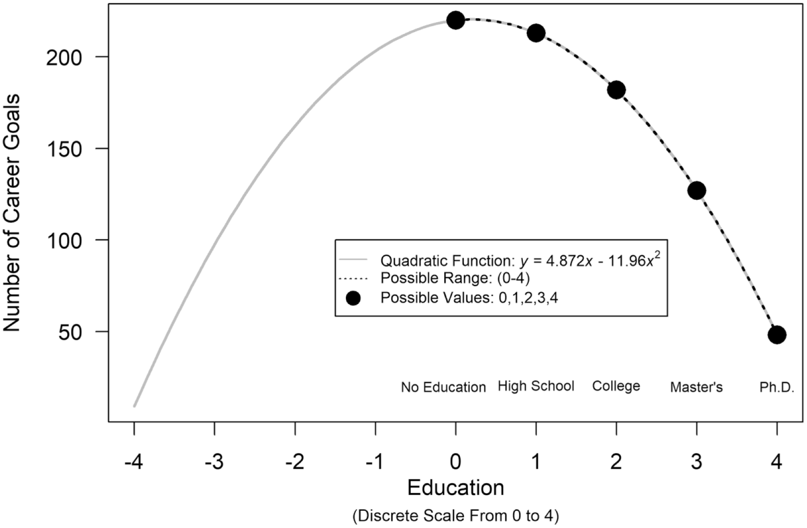
Hypothetical example of a significant quadratic term not associated with an actual U shape. Number of goals scored by soccer players during their careers is graphed as a function of the players’ educational achievement. Although the regression analysis yielded a quadratic function, the overall pattern is U shaped only if impossible values of x are included. The R code to reproduce this figure is available at https://osf.io/9uwxg/.

Level 2: Is the sign flip within the range of values?

At the next level, a quadratic regression is interpreted as providing evidence for a U-shaped relation only if the estimate of b is statistically significant within the range of observed, or at least possible, x values. Some researchers have carried out this additional step in their published articles (it is also illustrated by the preceding discussion of Fig. 1). For example, Berman, Down, and Hill (2002) wrote, “The value [at which the sign flips] is actually above any value observed in the data, suggesting that, although negative returns are a theoretical possibility, they are not encountered” (p. 23). Even with this step, however, it is problematic to conclude that the relationship is U shaped, because we need to take into account sampling error. We assume that the true relationship is y = ax + bx², but we do not observe a and b and instead observe estimates $\hat{a}$ and $\hat{b}$ . As estimates, they contain error, and therefore, our estimate of the point at which the effect of x on y flips sign, $(- \hat{a} / 2 \hat{b})$ $\hat{b}$ , also contains error.⁷

Level 3: Is the sign flip statistically significant within the range of values?

Noting that a quadratic term is simply an interaction of a variable with itself (see, e.g., McClelland & Judd, 1993, p. 382), we can take into account sampling error in analyses of quadratic regression estimates in general, and in analyses of the point where the effect of x on y flips sign in particular, as we do for any regression interaction. In particular, we may estimate the effect of x on y, and its confidence interval and/or p value, for different values of x. This general approach to analyzing interactions was first introduced by Johnson and Neyman (1936). It is sometimes known as the pick-a-point or spotlight approach when applied to a handful of x values, and as the floodlight, or Johnson-Neyman, procedure when applied to all of them or to the critical x values where the slope changes between being statistically significant and not being statistically significant (Aiken & West, 1991; Preacher, Curran, & Bauer, 2006; Spiller, Fitzsimons, Lynch, & McClelland, 2013). In recent years, a few articles have explicitly suggested relying on this Johnson-Neyman procedure to analyze quadratic-regression result when testing for U-shaped relationships (Lind & Mehlum, 2010; Miller, Stromeyer, & Schwieterman, 2013; Spiller et al., 2013).⁸

Even this more sophisticated use of quadratic regressions to test for a U shape is invalid, however. The reason is that the regression results, and therefore the Johnson-Neyman calculations, hinge on the assumption that the true relationship between x and y is exactly quadratic. Figure 2 provides realistic examples of cases in which the assumption is not met and the conclusions are erroneous.

Fig. 2.

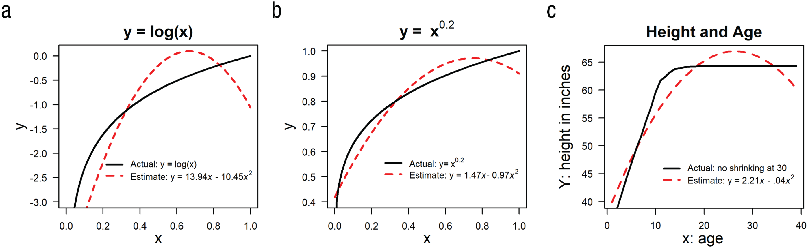
Examples of quadratic regressions misdiagnosing presence of a U shape. The graphs in (a) and (b) were created using a single simulated data set with N = 100,000; for each graph, the values of x were obtained by squaring random draws from the U(0,1) distribution. Large samples without noise were used to convey the point that quadratic regressions get it wrong because of specification error, rather than, say, lack of power or sampling error. The data in (c) come from the Centers for Disease Control (Kuczmarski, 2002). The R code to reproduce this figure is available at https://osf.io/3psev/.

Figure 2a shows a scenario in which the true relationship is y = log(x) and a quadratic regression would result in $\hat{y}$ = 13.94x – 10.45x². In this equation, the effect of x on y is, dy/dx = 13.96 – 2 * 10.45x. When x = 0.25, the effect of x is positive, 8.735, but in contrast, when x = 0.75, the effect is negative, −1.71. Of course, that result is wrong, as the effect of x is never negative when y = log(x), but it is estimated as negative because we are incorrectly assuming that the relationship is quadratic. Specification error is behind the erroneous conclusion. Figures 2b and 2c provide additional examples of quadratic regression leading to misdiagnosis of a U-shaped relationship.

Assuming a quadratic relationship may also lead to false negatives, failure to diagnose U-shaped relationships that are present, even when the sample size is infinite. This will occur when the true relationship is U shaped but deviates sufficiently from the quadratic shape (see Fig. 3).

Fig. 3.

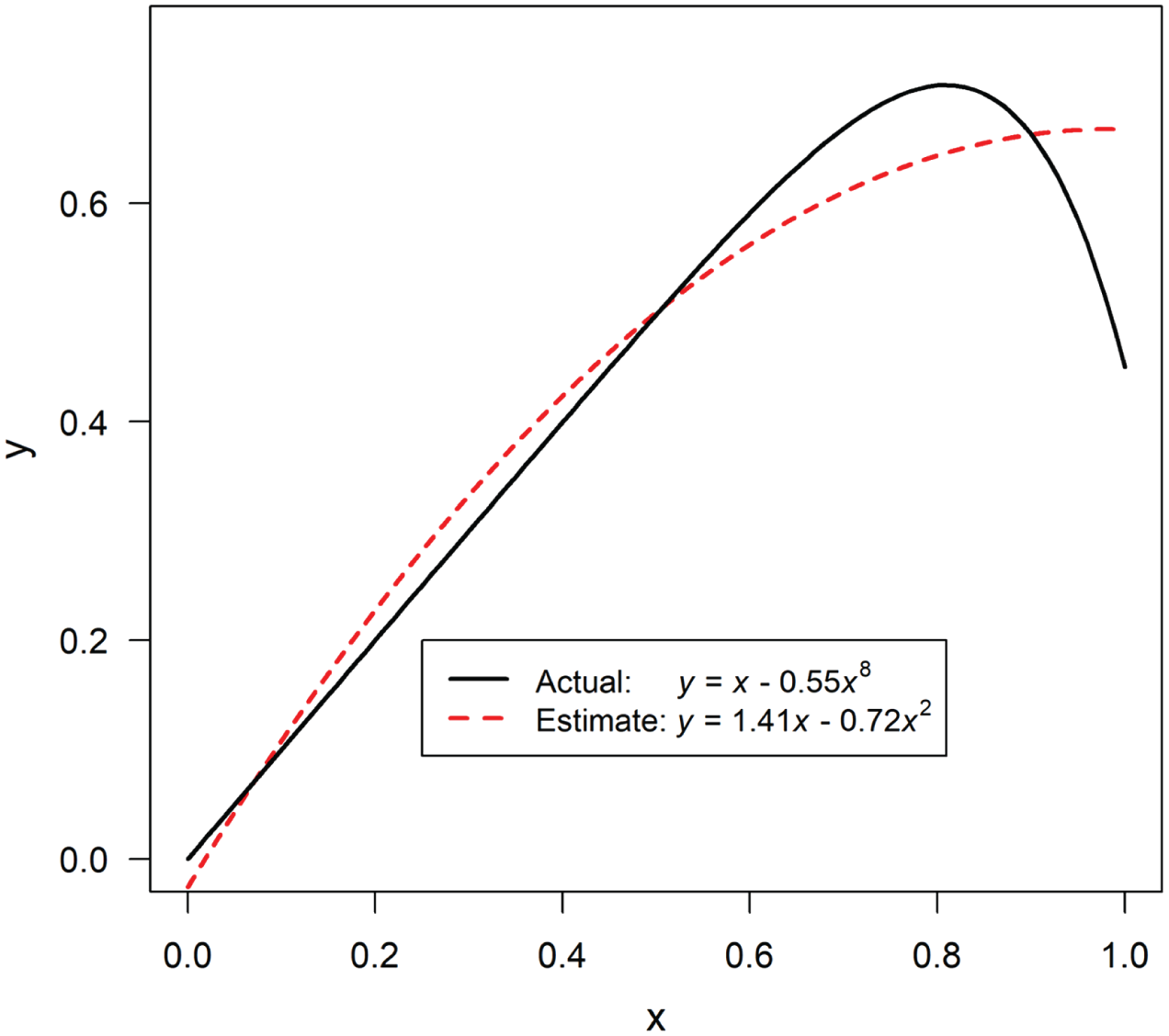
Example of a quadratic regression that falsely indicates the absence of a U shape. The graph was created from a single data set with N = 100,000 observations; x was generated by drawing at random from the U(0,1) distribution and squaring the result. The R code to reproduce this figure is available at https://osf.io/3psev/.

The quadratic regressions in Figures 2 and 3 perform poorly because they minimize the sum of squared errors, ( $\hat{y}$ – y)² without taking into account overall shape. During the model-fitting process, there is no penalty if obtaining a better fit requires outputting a quadratic function that generates a nonexistent U shape or misses a real U shape.

What About Diagnostic Tests?

Many textbooks recommend that researchers conduct diagnostic tests before interpreting regression results, but are those recommendations enough to protect us from wrong inferences about U shapes based on quadratic regressions? In this section, I argue that the answer is no.

First, in practice, researchers do not follow the recommendations; they do not run, or at least do not report, diagnostic tests on their regression results. Second, regression diagnostics qualitatively assess the general adequacy of the model, but we want to quantitatively assess the adequacy of the conclusion that the relationship is U shaped. Figure 4 illustrates this problem, showing a case in which regression diagnostics for a true-positive and a false-positive U-shaped relationship are indistinguishable from one another.

Fig. 4.

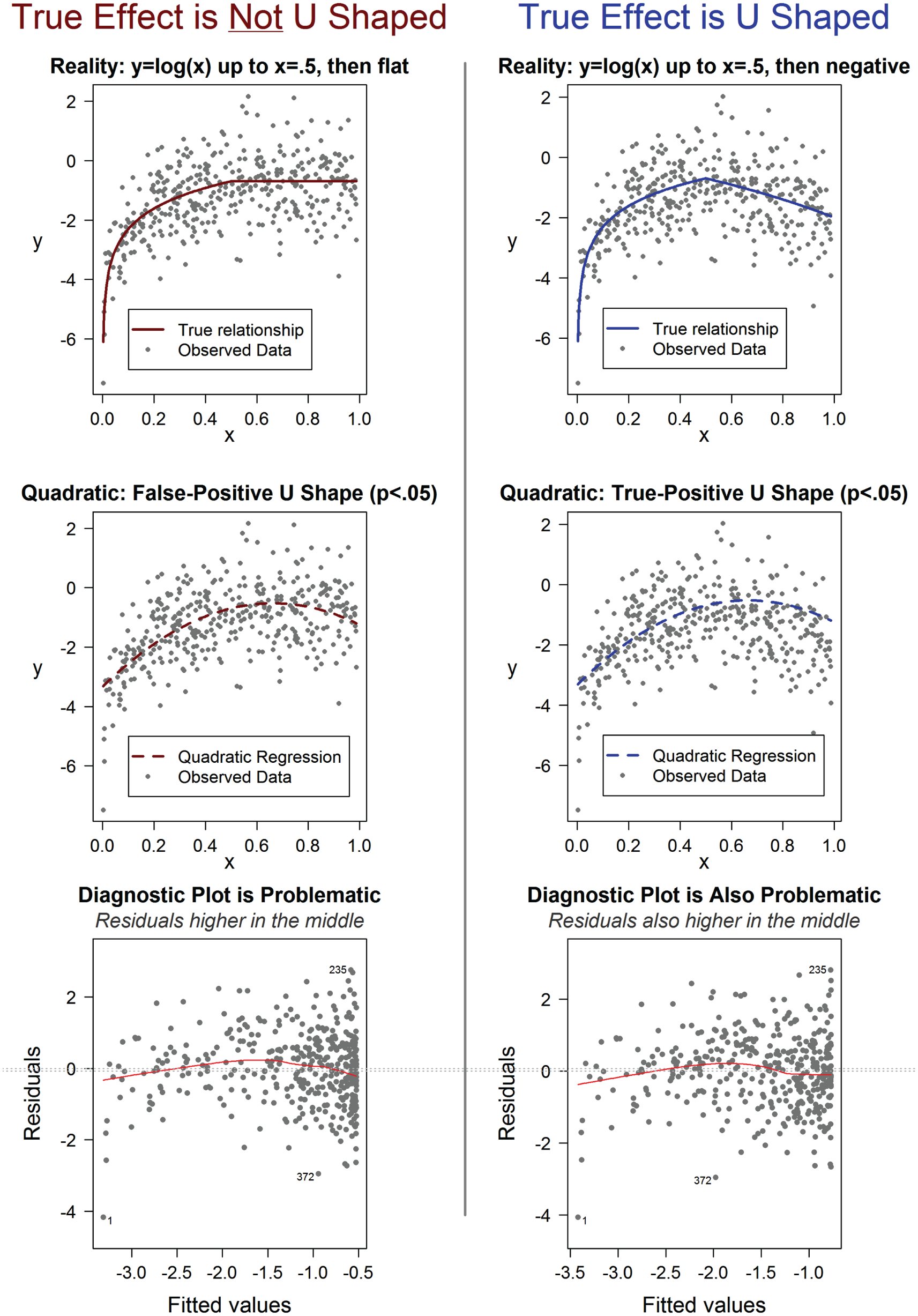
Example illustrating that diagnostic plots are not diagnostic about the correctness of an inference about a U-shaped relationship based on quadratic-regression results. The data for this example were generated by drawing 400 observations from a U(0,1) distribution for x and adding noise from an N(0,1) distribution to the true y value. The true relationship for the data in the left column is not U shaped, but the true relationship for the data in the right column is U shaped (see the models in the top row). The second row shows the results from a quadratic regression for each data set. In the third row, the residuals are plotted against fitted values; in the absence of specification error, there should be no association between the two, but the fitted (red) lines in the graphs show that the residuals are higher in their middle range than at lower and higher values. The R code to reproduce this figure is available at https://osf.io/kuj3d/.

Third, it is not clear what researchers should do when they diagnose their quadratic regression as misspecified. If not a quadratic model, what model should they estimate? There is no default alternative; researchers would need to try multiple functional forms (e.g., higher-order polynomials, interrupted log regressions, various interactions) until one subjectively seems to fit well enough. This leads to two problems. One is that when those more complicated models are estimated, it is not clear how the researcher should go about testing for a U shape. For example, if we fit a fourth-order polynomial to the y = log(x) data used to construct Figure 2a, we obtain the following estimate: y = 44x – 142x² + 189x³ – 86x⁴. Should we interpret this equation as evidence for or against a U shape? Perhaps the most sensible thing to do is to compute the implied marginal effect of x on y for every value of x and then average the resulting values for two ranges of x. But now we have a two-lines test, except that we are averaging fitted values, computed assuming an arbitrary functional form, instead of averaging observed values. In addition, the second problem is that the abundance of alternatives to the quadratic opens the door to overfitting in general and p-hacking in particular.

The Two-Lines Solution

Interrupted regression

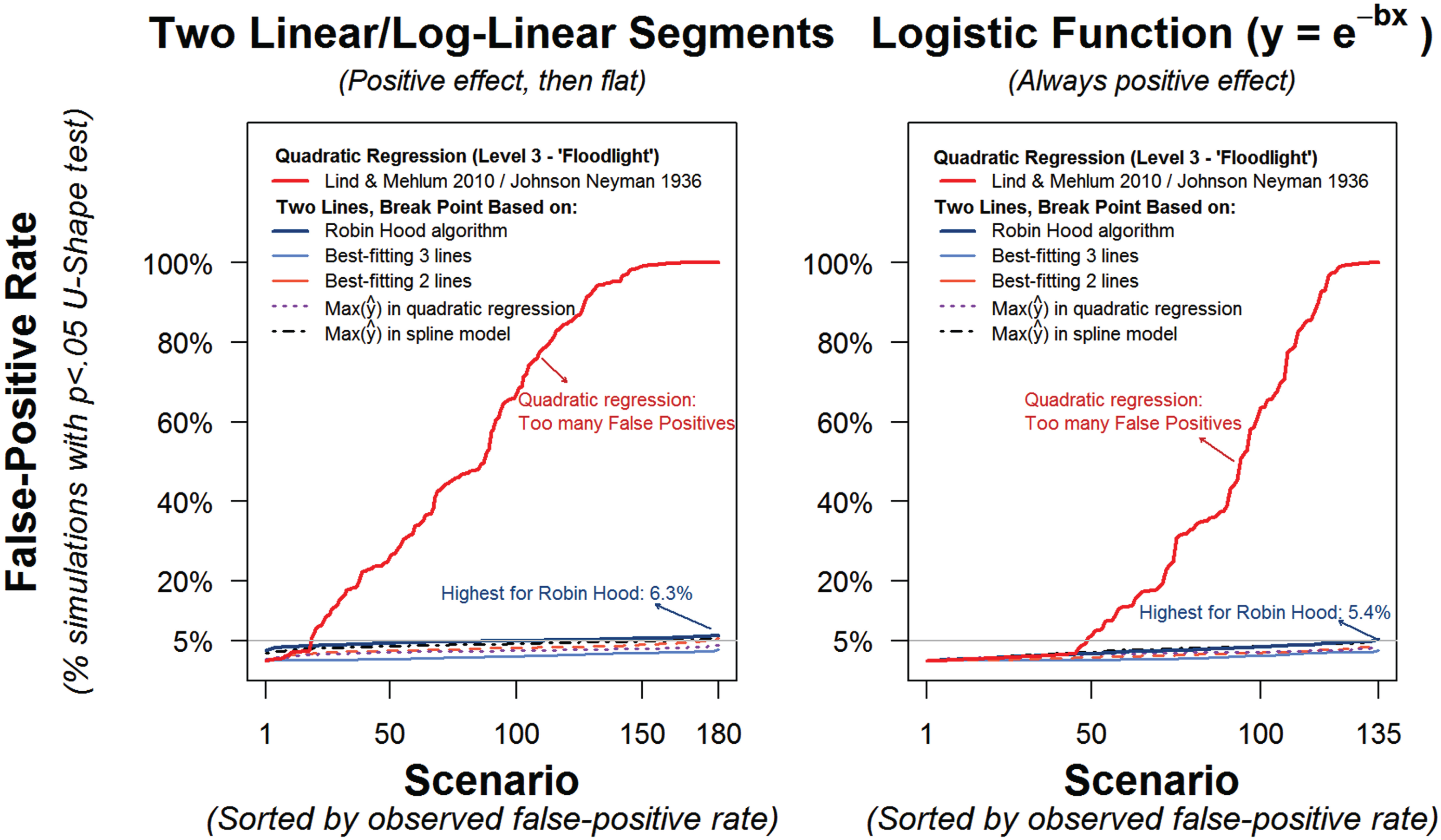
Because hypotheses positing U shapes state merely that the effect of x on y changes sign for low versus high x values, we should test these hypotheses by merely testing if the effect of x on y changes sign for low versus high x values. Such a test involves computing two average slopes, which in turn is done by estimating two regression lines, one for x ≤ x_c and the other for x ≥ x_c, where x_c is the break point separating the two regions. One may increase statistical efficiency by simultaneously estimating both lines in a single regression, relying on what is often referred to as an interrupted regression (see, e.g., Marsh & Cormier, 2001, p. 7). Specifically, interrupted regressions conform to the following general formulation:⁹

y = a + b x_{l o w} + c x_{h i g h} + d * h i g h + Z B_{Z},

(1)

where x_low = x – x_c if x < x_c and 0 otherwise, x_high = x – x_c if x ≥ x_c and 0 otherwise, and high = 1 if x ≥ x_c and 0 otherwise.

Z is the (optional) matrix with covariates, and B_Z is its vector of coefficients.

Setting the break point

We can set the break point seeking to maximize fit or to maximize statistical power. That is, we can seek to arrive at a model that fits the data best or at a model that has the highest probability of diagnosing f (x) as U shaped when it is, without exceeding the nominal false-positive rate when it is not.

Maximizing fit

Setting the break point to maximize fit involves answering this question: Given that we will fit the data with two lines, which break point leads to two lines that best fit the data overall? There is a literature examining how to maximize fit for segmented and interrupted regressions (see, e.g., Hansen, 2000; Molinari, Daures, & Durand, 2001; Muggeo, 2003; Stasinopoulos & Rigby, 1992). But when testing for U shapes we are not trying to fit the data as well as possible.

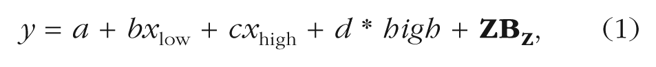
We are not fitting two lines with a possible discontinuity between them because we believe the real relationship has that shape and we want to approximate it as well as possible. Rather, we are only estimating regressions to compute average slopes in two sets of x values. Thus, we want to find the break point that answers a different question: If the true relationship is U shaped (i.e., if there really is a sign change for the effect of x on y within the set of observed values), which break point maximizes the chance that we will detect it? Figure 5 illustrates the conflict between these two goals. Moreover, later on, when evaluating the performance of different break points, I show that the break point that maximizes fit provides lower statistical power than that obtained with the proposed Robin Hood procedure.

Fig. 5.

Examples illustrating that the break point that maximizes overall two-lines fit does not necessarily maximize power to detect a U-shaped relationship. Each graph shows the best-fitting two-lines model (obtained using Muggeo’s, 2003, procedure) and the real relationship for a simulated data set. The vertical dotted lines contrast the break point for the two regression lines that maximizes overall fit and the break point at which the sign of the effect of x on y changes (i.e., the U-shape break point). The R code to reproduce this figure is available at https://osf.io/w3m2u/.

Maximizing power

Without making strong assumptions about (a) the functional form of the relationship between x and y, f (x); (b) the distribution of x; and (c) the distribution of the error term, it does not seem possible to arrive at a theoretically optimal break point that maximizes statistical power for U-shape testing. The approach I propose here, instead, is algorithmic, designed to have high power, rather than demonstrably maximal power, for a very broad range of situations (but presumably not all). I developed the algorithm keeping in mind three key ideas: (a) Because the two-lines test requires both slopes to be significant, increasing its power requires increasing the power of the statistically weaker of the two lines. A segment of an interrupted regression, in turn, has more power when (b) it is steeper (i.e., the effect is bigger) and (c) it includes more observations (i.e., the standard error is smaller). Thus, conceptually, the algorithm sets a break point that will increase the statistical strength of the weaker of the two lines, by placing more observations in that segment without overly attenuating its slope. I refer to it as the Robin Hood algorithm, for it takes away observations from the more powerful line and assigns them to the less powerful one.

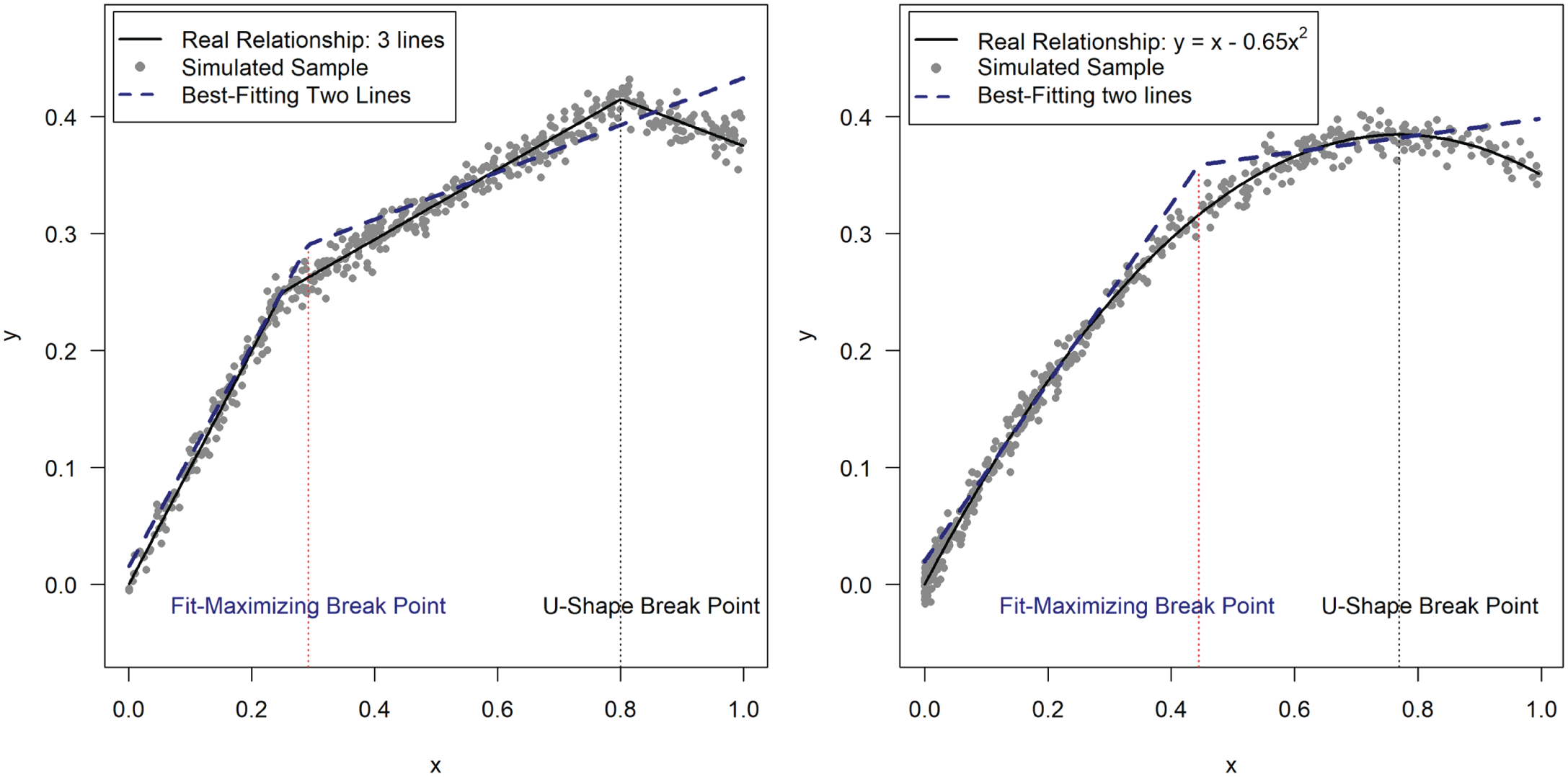
I rely on Figure 6 to describe the Robin Hood algorithm. Every panel involves the same true underlying relationship between x and y, depicted by the solid line in Figure 6a, and the same single random sample, depicted with the same scatterplot in every panel. From left to right, the top row in the figure illustrates increasingly sophisticated approaches for setting the break point, culminating in the proposed Robin Hood algorithm in the rightmost column. The bottom row shows the resulting two-lines regression estimates.

Fig. 6.

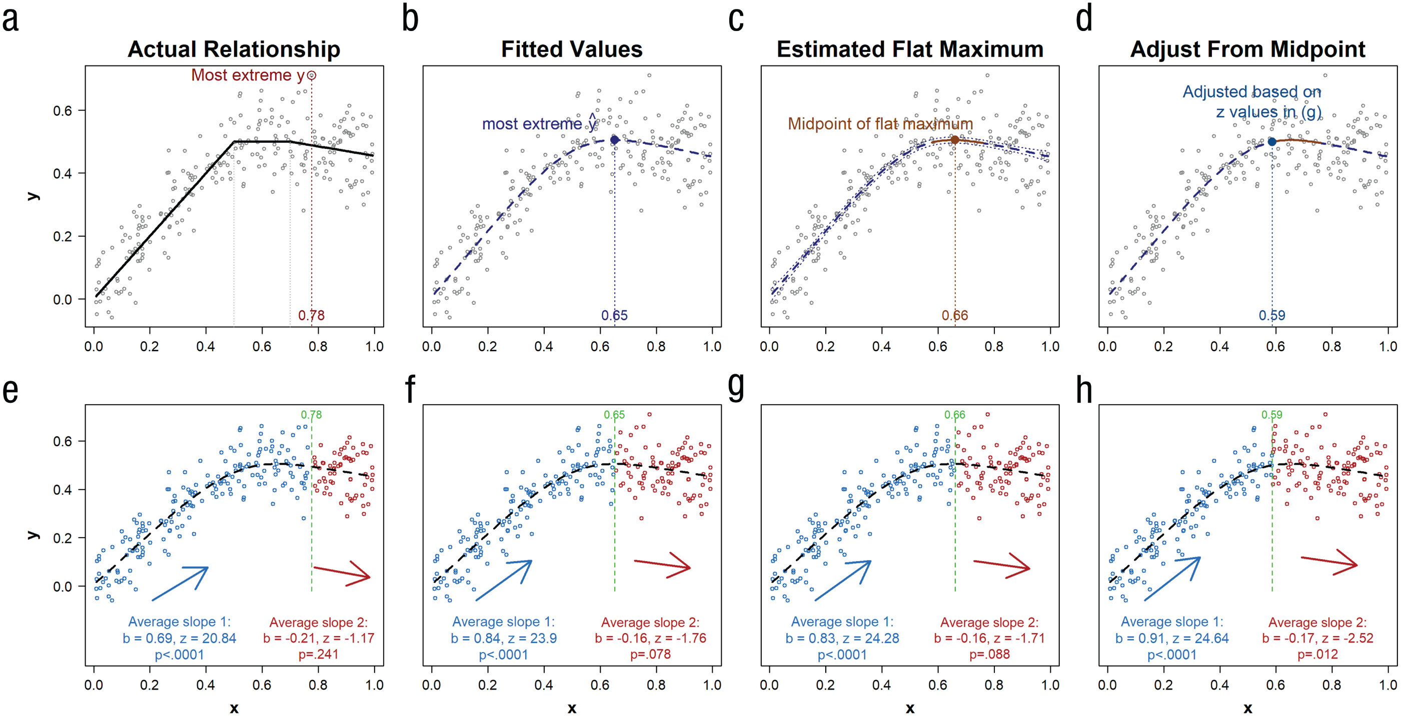
Illustration of four procedures to identify the break point (a–d) and their consequences (e–h). All panels are based on the same random sample (each circle represents a data point); the true relationship between x and y is shown by the solid line in (a). The effect of x on y is positive up to x = 0.5, flat up to x = 0.7, and negative onward. The top row shows four alternative ways to set the break point: It may be the x value associated with (a) the most extreme y value; (b) the most extreme fitted value, $\hat{y}$ ; (c) the midpoint of the flat maximum; or (d) the solution provided by the Robin Hood algorithm. The bottom row shows the resulting two-lines regressions. The fitted values in (b) through (d) were obtained by smoothing the scatterplot with a cubic spline. The flat region in (c) and (d) is where $\hat{y} s$ are within 1 SE of the maximum $\hat{y}$ . The R code to reproduce this figure is available at https://osf.io/zdert/.

For illustrative purposes, consider attempting to obtain two steep slopes by setting x_c, the break point, at the x value associated with the most extreme observed y value (first column in Fig. 6). An obvious problem is that individual observations, especially the most extreme one, can be greatly influenced by random error. Figure 6a, for example, shows that the x value associated with the most extreme observation, x = 0.78, falls outside the range of x values with maximum true y values, 0.5 < x < 0.7.

We can cancel much of the random error by estimating a flexible model of f (x), for example, a polynomial, local, kernel, or spline regression, and using the model’s fitted values instead of the observed values to identify the most extreme observations. I rely on splines here because they easily accommodate covariates, can be used to construct confidence intervals for f (x), and do not rely on functional-form assumptions (see Section 3.2.1 in Wood, 2006).¹⁰ In particular, Figures 6b and 6f depict the fitted values, $\hat{y}$ s, obtained from a cubic spline regression and showcase the consequences of moving the break point from the x associated with the most extreme observed y to the x associated with the most extreme fitted value, $\hat{y}$ _max.

In the example depicted in Figure 6, and presumably in many psychological phenomena, relationships are U rather than V shaped, having regions with a relatively flat maximum. It therefore seems sensible to identify the set of most extreme $\hat{y}$ s rather than the single most extreme $\hat{y}$ . I define $\hat{y}$ s within 1 SE of $\hat{y}$ _max as that set and refer to it as $\hat{y}$ _flat. Thus, every $\hat{y}$ in $\hat{y}$ _flat is within 1 SE of $\hat{y}$ _max. The solid line in Figure 6c depicts $\hat{y}$ _flat, and Figure 6g shows the slopes of the two resulting regression lines when the break point is set as the midpoint of $\hat{y}$ _flat.

We now have a set of candidate x_c values, those associated with $\hat{y}$ _flat. The goal is to choose the one among them that we expect to result in the highest statistical power to detect a U shape, and thus the one among them that we expect to give the highest statistical power to the weaker of the two lines within the interrupted regression. The algorithm achieves that goal by setting x_c so that it allocates a disproportionate share of the observations in $\hat{y}$ _flat to the weaker line; by increasing the number of observations in that segment, it reduces its standard error, increasing its statistical power.

The algorithm proceeds in two steps. In the first step, it identifies which of the two lines is statistically weaker. In the second step, it sets the break point by allocating observations in $\hat{y}$ _flat to the first versus second line in inverse proportion to the lines’ relative statistical strength. Specifically, in the first step, the algorithm sets the x value that is the midpoint of $\hat{y}$ _flat as an interim break point. It estimates an interrupted regression and computes the absolute values of the test statistics for both lines, z₁ and z₂, and then sets the break point for the second step in inverse proportion to these zs. Specifically, the break point becomes the z₂/(z₁ + z₂)th percentile of the x values within $\hat{y}$ _flat.

If both lines are about equally strong, statistically speaking, with roughly identical test statistics, the break point will remain roughly at the midpoint of $\hat{y}$ _flat. If the z value of the first line in the first step were, say, 3 times that of the second line, then the break point would be set at the 75th percentile of xs within $\hat{y}$ _flat, so that the second (weaker) line has 75% of $\hat{y}$ _flat and the first line the remaining 25%. Again, the algorithm allocates additional observations from within the $\hat{y}$ _flat region to the weaker line so that its standard error gets smaller.

In Figure 6, setting the midpoint of $\hat{y}$ _flat as the break point leads to z₁ = 24.28 and z₂ = 1.71. Computing the ratio z₂/(z₁ + z₂), we obtain 6.58%, so the Robin Hood algorithm sets the breakpoint at the 6.58th percentile of the x values associated with $\hat{y}$ _flat, which in that sample corresponds to x = 0.59 (Fig. 6d). Using that break point, we obtain the final interrupted regression to test for the presence of a U shape (see Fig. 6h), and in this case, we obtain a much stronger result for the second slope, p = .012 (vs. p = .088).

In sum, the Robin Hood algorithm consists of the following five steps:

Estimate a cubic spline for the relationship between x and y

Identify $\hat{y}$ _max, the most extreme internal fitted value

Identify $\hat{y}$ _flat, the set of $\hat{y}$ values within 1 SE of $\hat{y}$ _max

Estimate an interrupted regression using as the break point the median x value within $\hat{y}$ _flat (The regression will result in two test statistics, one for each line. Let their absolute values be z₁ and z₂.)

Set the break point at the z₂/(z₁ + z₂)th percentile of the x values associated with $\hat{y}$ _flat

It is important to note that because the break point is set algorithmically within a set of candidate break points, it conveys no interpretable meaning on its own. We should not conclude that the breakpoint is the point where the sign of the effect switches. The specific point of the sign switch, to the extent it actually exists, is not estimated precisely with the two-lines test.

Performance of the Two-Lines Test

False-positive and false-negative U shapes

Figure 7 shows results for false-positive detection of a U shape in simulated scenarios. The left panel shows results obtained with six testing procedures (including the Robin Hood algorithm) when the true relationship would be expected to lead to the most false positives: an initial strong effect followed by a long flat segment. The right panel shows results for the same testing procedures for scenarios in which the data followed a (monotonic) logistic function. For the quadratic-regression approach, I report results for its most sophisticated version, the procedure proposed by Lind and Mehlum (2010), which is equivalent to that proposed by Spiller et al. (2013), Miller et al. (2013), and Aiken and West (1991).¹¹

Fig. 7.

False-positive rates for detecting U shapes in simulated data sets. Results are shown for six different testing procedures, including quadratic regression and the two-lines test with the Robin Hood algorithm. Results in the left panel are for scenarios involving a relationship between x and y that consisted of two segments. For x < x_c, the marginal effect of x on y was positive; for x ≥ x_c, it was zero. The scenarios combined the following parameterizations: (a) five distributions of x (normal, uniform, beta with left skew, beta with right skew, or optimized for the quadratic as in McClelland, 1997), (b) two effects of x on y (y = x or y = log(x); i.e., linear or log linear), (c) three sample sizes (100, 200, or 500), (d) three values of σ in e~N(0,σ) (100%, 200%, or 300% of SD(y) before adding noise), and (e) two values of x_c (30th or 50th percentile of x). The full combination of parameters led to 180 scenarios. Results in the right panel are for scenarios involving a logistic function. The same parameterizations for the distribution of x, sample size, and amount of noise as in the left panel were used, but instead of differing in slopes and cutoffs, the scenarios differed in the values of b in the logistic function (0.5, 1.5, or 2.5). Thus, there were 135 scenarios in total. All two-lines results are from interrupted regressions (i.e., regressions that allowed a discontinuity at the break point). Each scenario was simulated 500 times, and if the observed false-positive rate was 4.5% or higher, it was run another 5,000 times. The R code to reproduce the simulations is available at https://osf.io/wdbmr/.

The results in Figure 7 are highly consistent. They show that the quadratic-regression approach to testing for U-shaped relationships had an unacceptably high false-positive rate—often a 100% rate—for a very broad range of scenarios. In contrast, the two-lines approach in general, and the Robin Hood procedure for setting the break point in particular, showed acceptable performance. False-positive rates were typically below the nominal 5% level (as is typically the case when the null hypothesis is a composite null; see, e.g., Bowman, Jones, & Gijbels, 1998), and even the post hoc most extreme scenario raised the false-positive rate only barely above the 5% level (and these rates are necessarily overestimates, as they were selected ex post because they were the highest values).

Exploring factors that influence false-positive rates (see Supplement 1 in the Supplemental Material), I found that scenarios using the distribution of x suggested by McClelland (1997) had higher false-positive rates than other scenarios; greater levels of random noise were also associated with higher false-positive rates. I ran additional simulations that relied on that distribution of x and had even higher levels of noise than those used in Figure 7 and found that the false-positive rate did not increase any further.

Figure 8 moves on to false negatives, comparing estimates of statistical power obtained using the Robin Hood algorithm to set the break point with estimates of power obtained using four alternative approaches to setting the break point. Results are shown for two general functional forms (Fig. 9 shows examples of the individual simulations behind the left panel of Fig. 8). Because quadratic regressions yielded unacceptably high false-positive rates, Figure 8 does not include power results for that approach. For statistical inference, we should select the most powerful test among those that satisfy the nominal false-positive rate. For example, if the test consisted of a coin that read “U shape” on either side, flipping the coin would lead to 100% power, but this is not a statistical test we would want to use.

Fig. 8.

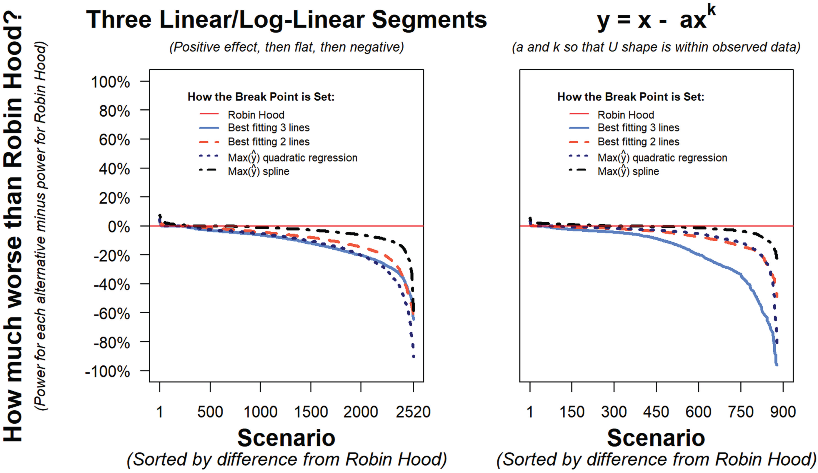
Statistical power for detecting U shapes: how the Robin Hood algorithm compares with four alternative approaches to setting the break point. Results in the left panel are for simulated scenarios involving three linear or log-linear segments, with cutoffs at x_c and x_d. For x < x_c, the marginal effect of x on y was positive; for x_c < x < x_d, the marginal effect of x was zero; and for x > x_d, the marginal effect was negative. The scenarios combined the same parameters as in the left panel of Figure 7, crossed with four values of x_d (30th, 50th, 70th, or 90th percentile of x) and four values of the slope of the negative effect of x on y when x > x_d (25%, 50%, 100%, or 200% of the magnitude of the slope when x < x_c). The full combination of parameters led to 2,520 scenarios (see Fig. 9 for examples). Results in the right panel are for simulated scenarios following the form y = x – ax^k. The same parameterizations for the distribution of x, sample size, and amount of noise as in the left panel were used, but instead of differing in slopes and cutoffs, the scenarios differed in the values of k (k = 2, 3, 4, or 5) and the values of a (set so that y = x – ax^k would produce an inverted U shape with the maximal value of y at the 50th, 60th, 70th, 80th, or 90th percentile of x). The full combination of parameters led to 900 scenarios. Results for each of the 3,420 scenarios are based on 500 or 2,500 simulations, depending on the extremity of results after 500. 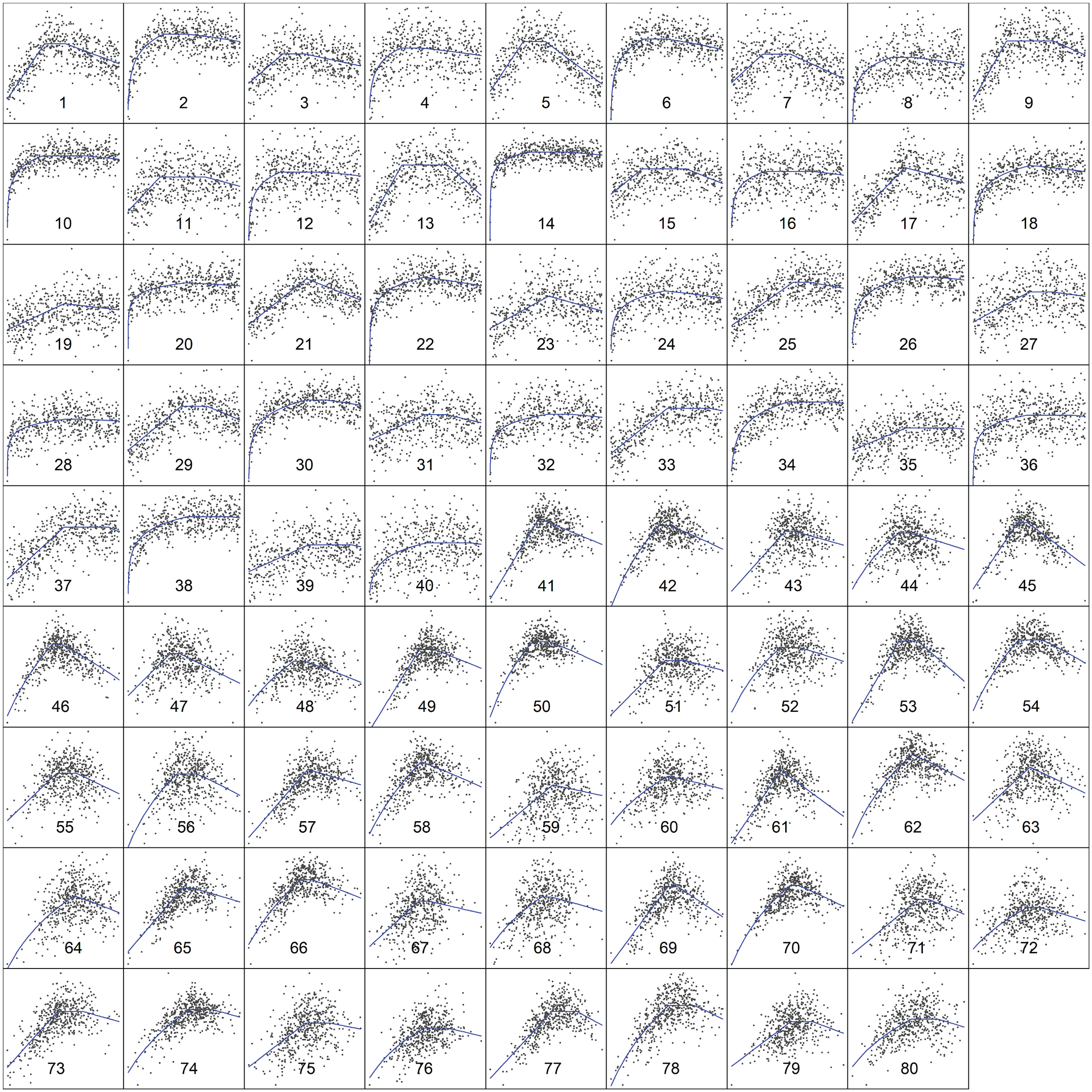Max( $\hat{y}$ ) = the highest fitted value of y. The R code to reproduce the simulations is available at https://osf.io/wdbmr.

Fig. 9.

A representative subset of 80 of the 2,520 scenarios used to compare power across procedures in the left panel of Figure 8. The solid lines represent the underlying true functions, and each gray dot represents a single random draw from the specified distributions of x values and noise. Max( $\hat{y}$ ) = the highest fitted value of y. The R code to reproduce this figure is available at https://osf.io/m7avc/.

To facilitate comparisons with the proposed Robin Hood procedure, Figure 8 shows the difference between the power of each alternative procedure and that of the Robin Hood procedure. The panels of Figure 8 paint a highly consistent picture. The Robin Hood algorithm generally outperformed all other alternatives. Two counterintuitive general patterns are worth highlighting. First, estimating three rather than two lines led to dramatic losses of statistical power; this occurred because the observations allocated to the middle line did not contribute to the precision of the slope estimates involved in the test. Second, the least powerful approach to setting the break point for a two-lines estimation was an approach previously proposed by several authors, including me: setting the break point as the quadratic regression’s most extreme fitted value (Haans, Pieters, & He, 2016; Iribarren et al., 1996; Simonsohn & Nelson, 2014).

Demonstrations

In this section, I take two examples of purportedly U-shaped relationships in the published literature and demonstrate that using the two-lines test instead of a quadratic regression would lead to different conclusions. The top row in Figure 10 revisits the analyses by Sterling, Jost, and Pennycook (2016), who wrote (in their discussion of secondary analyses), that people “who were moderate in terms of their support for the free market appeared to be more susceptible to bullshit than extremists in either direction” (p. 356). They arrived at this conclusion that an inverted-U-shaped relationship was present because the quadratic term in their regression was significant (p = .026). I successfully reproduced their results analyzing their posted data (Fig. 10a). The two-lines test, however, showed that the slope of the second line, although negative, was far from significant, p = .45 (Fig. 10b). Keep in mind that if x and y were uncorrelated for high values of x (i.e., if the true second slope were flat), 50% of the estimated slopes would be negative (and 45% of them would be at least as steep as observed—that is the meaning of the p = .45 reported in the figure). The data are inconclusive: They are consistent with a U-shaped relationship, consistent with lack of a correlation among people who endorse free-market ideology at a relatively high level, and consistent with a monotonic effect. Again, prediction of a U-shaped relationship was secondary to the authors. Their core prediction of an association between free-market ideology and bullshit receptivity is consistent with the first line in the two-lines test).

Fig. 10.

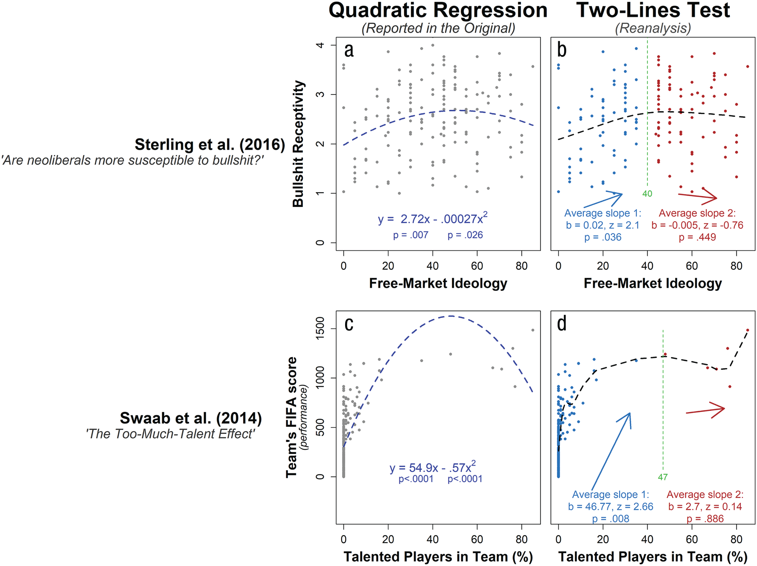
Examples of the difference in results obtained when quadratic regression and the two-lines test are applied to data from published articles. The graphs in the top row (a, b) show results for Sterling, Jost, and Pennycook’s (2016) study on the relationship between ratings of the profundity of a series of vague but seemingly profound statements and endorsement of free-market ideology. The graphs in the bottom row (c, d) show results for Swaab, Schaerer, Anicich, Ronay, and Galinsky’s (2014) study of the relationship between a country’s ranking by the Fédération Internationale de Football Association (FIFA) and the percentage of players on the country’s team who played for a top professional team (e.g., Arsenal). Dots depict individual observations (experimental subjects and country teams in the top and bottom rows, respectively). The horizontal dashed lines depict fitted lines from quadratic regressions in the left column and fitted lines from cubic splines in the right column. The R code to reproduce this figure is available at https://osf.io/3jbzk/.

Swaab, Schaerer, Anicich, Ronay, and Galinsky (2014), in their Study 2, examined the relationship between the number of elite players on a country’s soccer team and its rating by the Fédération Internationale de Football Association (FIFA). Their results, they wrote, “revealed a significant quadratic effect of top talent: Top talent benefited performance only up to a point, after which the marginal benefit of talent decreased and turned negative” (p. 1584; italics added). I successfully replicated those results with independently obtained data, but in the two-lines test, the slope of the second line was also positive (albeit far from significant; see Fig. 10b). These data do not support the conclusion that there is such a thing as “too much talent” in international soccer teams.

Limitations

In this section, I discuss three limitations of the two-lines test and the proposed Robin Hood algorithm.

Limitation 1: asymptotic properties

I have proposed an algorithm and evaluated its performance via simulation in small samples, without deriving its theoretical asymptotic properties. Moreover, the two-lines test uses this algorithm without known theoretical properties to set the break point.

Limitation 2: X, N, and W shapes

The two-lines test is expected to perform well as long as the true relationship of interest has at most two regions where the impact of x on y has opposite signs; that is, the relationship is (a) flat overall (no effect), (b) monotonic or weakly monotonic, or (c) U shaped. It will not perform well, at least in terms of interpretability, if the true relationship has more than one change in sign, for instance, if it is N shaped, X shaped, or W shaped, rather than U shaped. Such relationships, it is worth noting, invalidate the interpretability of quadratic regressions as well. The nonparametric smooth line that accompanies the output generated by the app that runs the two-lines test (available at http://webstimate.org/twolines/) may be used as a partial solution to this limitation, as it alerts users if the relationship looks N, X, or W shaped.

Limitation 3: imprecise false-positive rate

The precise false-positive rate of the two-lines test is not known, and it cannot be guaranteed to be 5% for any specific data set, for two reasons. The first reason is that the null hypothesis of the absence of a U shape is what is known as a composite null. The second reason is that the Robin Hood algorithm slightly overfits the data. For a detailed discussion of these issues, see Supplement 8 in the Supplemental Material. Nevertheless, the false-positive rate of the two-lines test is expected to be generally lower than the nominal rate, and almost never higher than 6% for a nominal α of 5% (see Fig. 7 and also Supplement 1 in the Supplemental Material).

Conclusions

The use of quadratic regressions to test for U-shaped relationships is as invalid as it is common. To interpret the results of a quadratic regression, we need to know that the true functional form is indeed quadratic—something that is virtually impossible to know in social science. The two-lines test is arguably the most straightforward test of the hypothesis that the average effect of x on y is of opposite sign for high versus low values of x. It makes no assumptions about the functional form of f (x). The Robin Hood procedure to set the break point for the two lines achieves notably higher power than any alternative with which I have compared it.

Supplemental Material

SimonsohnOpenPracticesDisclosure – Supplemental material for Two Lines: A Valid Alternative to the Invalid Testing of U-Shaped Relationships With Quadratic Regressions

Supplemental material, SimonsohnOpenPracticesDisclosure for Two Lines: A Valid Alternative to the Invalid Testing of U-Shaped Relationships With Quadratic Regressions by Uri Simonsohn in Advances in Methods and Practices in Psychological Science

Supplemental Material

SimonsohnSupplementalMaterial – Supplemental material for Two Lines: A Valid Alternative to the Invalid Testing of U-Shaped Relationships With Quadratic Regressions

Supplemental material, SimonsohnSupplementalMaterial for Two Lines: A Valid Alternative to the Invalid Testing of U-Shaped Relationships With Quadratic Regressions by Uri Simonsohn in Advances in Methods and Practices in Psychological Science

Footnotes

Appendix

Table A1.

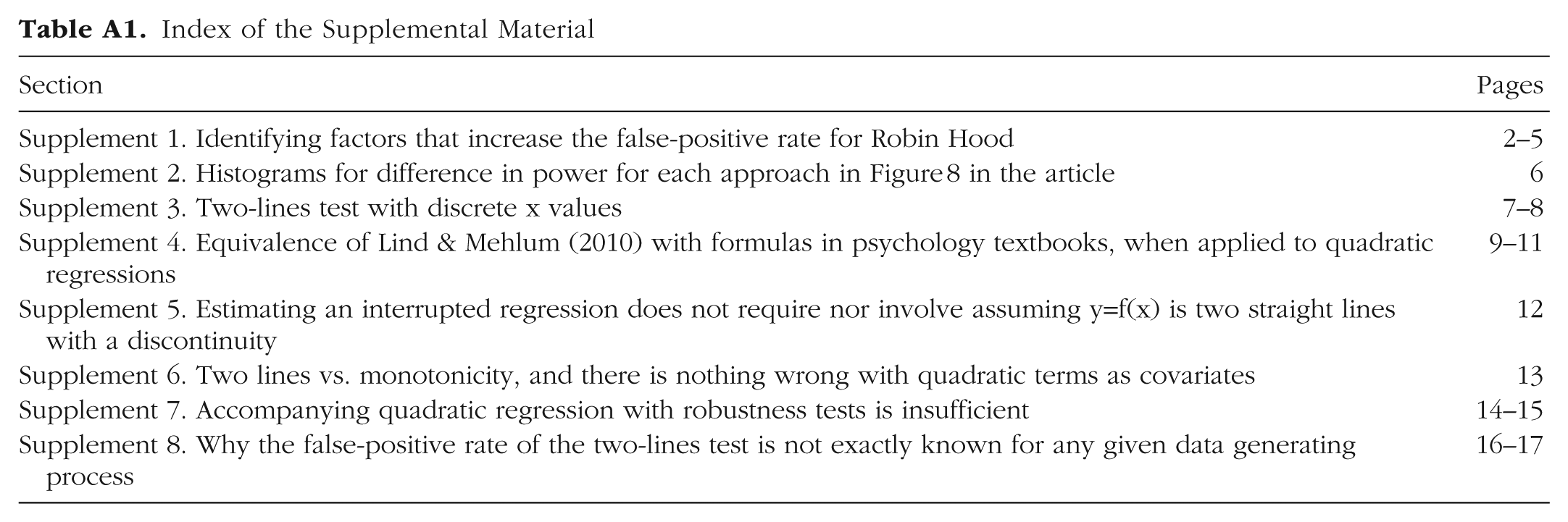
Index of the Supplemental Material

Section	Pages
Supplement 1. Identifying factors that increase the false-positive rate for Robin Hood	2–5
Supplement 2. Histograms for difference in power for each approach in Figure 8 in the article	6
Supplement 3. Two-lines test with discrete x values	7–8
Supplement 4. Equivalence of Lind & Mehlum (2010) with formulas in psychology textbooks, when applied to quadratic regressions	9–11
Supplement 5. Estimating an interrupted regression does not require nor involve assuming y=f(x) is two straight lines with a discontinuity	12
Supplement 6. Two lines vs. monotonicity, and there is nothing wrong with quadratic terms as covariates	13
Supplement 7. Accompanying quadratic regression with robustness tests is insufficient	14–15
Supplement 8. Why the false-positive rate of the two-lines test is not exactly known for any given data generating process	16–17

Action Editor

Daniel J. Simons served as action editor for this article.

Author Contributions

U. Simonsohn is the sole author of this article and is responsible for its content.

Declaration of Conflicting Interests

The author(s) declared that there were no conflicts of interest with respect to the authorship or the publication of this article.

Supplemental Material

Additional supporting information can be found at

Open Practices

All data and materials have been made publicly available via the Open Science Framework and can be accessed at https://osf.io/psfwz/. The complete Open Practices Disclosure for this article can be found at http://journals.sagepub.com/doi/suppl/10.1177/2515245918805755. This article has received badges for Open Data and Open Materials. More information about the Open Practices badges can be found at .

Notes

References

Aiken

L. S.

West

S. G.

(1991). Multiple regression: Testing and interpreting interactions. Thousand Oaks, CA: Sage.

Berman

S. L.

Down

Hill

C. W.

(2002). Tacit knowledge as a source of competitive advantage in the National Basketball Association. Academy of Management Journal, 45, 13–31.

Bowman

Jones

Gijbels

(1998). Testing monotonicity of regression. Journal of Computational and Graphical Statistics, 7, 489–500.

Choi

Kirkorian

H. L.

(2016). Touch or watch to learn? Toddlers’ object retrieval using contingent and noncontingent video. Psychological Science, 27, 726–736. doi:10.1177/0956797616636110

Cohen

West

S. G.

Aiken

L. S.

(2003). Applied multiple regression/correlation analysis for the behavioral sciences (3rd ed.). Mahwah, NJ: Erlbaum.

Gelman

Park

D. K.

(2008). Splitting a predictor at the upper quarter or third and the lower quarter or third. The American Statistician, 62(4), 1–8.

Grant

A. M.

Schwartz

(2011). Too much of a good thing: The challenge and opportunity of the inverted U. Perspectives on Psychological Science, 6, 61–76.

Haans

R. F.

Pieters

Z. L.

(2016). Thinking about U: Theorizing and testing U- and inverted U-shaped relationships in strategy research. Strategic Management Journal, 37, 1177–1195.

Hansen

B. E.

(2000). Sample splitting and threshold estimation. Econometrica, 68, 575–603.

10.

Iribarren

Sharp

Burchfiel

C. M.

Sun

Dwyer

J. H.

(1996). Association of serum total cholesterol with coronary disease and all-cause mortality: Multivariate correction for bias due to measurement error. American Journal of Epidemiology, 143, 463–471.

11.

Jaspers

Pieters

(2016). Materialism across the lifespan: An age-period-cohort analysis. Journal of Personality and Social Psychology, 111, 451–473. doi:10.1037/pspp0000092

12.

Johnson

P. O.

Neyman

(1936). Tests of certain linear hypotheses and their application to some educational problems. Statistical Research Memoirs, 1, 57–93.

13.

Josef

A. K.

Richter

Samanez-Larkin

G. R.

Wagner

G. G.

Hertwig

Mata

(2016). Stability and change in risk-taking propensity across the adult life span. Journal of Personality and Social Psychology, 111, 430–450. doi:10.1037/pspp0000090

14.

Koopmann

Lanaj

Wang

Zhou

Shi

(2016). Nonlinear effects of team tenure on team psychological safety climate and climate strength: Implications for average team member performance. Journal of Applied Psychology, 101, 940–957. doi:10.1037/apl0000097

15.

Kuczmarski

R. J.

Ogden

C. L.

Guo

S. S.

Grummer-Strawn

L. M.

Flegal

K. M.

Mei

. . . Johnson

C. L.

(2002). 2000 CDC growth charts for the United States: Methods and development (DHHS Publication No. (PHS) 2002-1696). Retrieved from https://www.cdc.gov/nchs/data/series/sr_11/sr11_246.pdf

16.

Lind

J. T.

Mehlum

(2010). With or without U? The appropriate test for a U-shaped relationship. Oxford Bulletin of Economics and Statistics, 72, 109–118.

17.

Loschelder

D. D.

Friese

Schaerer

Galinsky

A. D.

(2016). The too-much-precision effect: When and why precise anchors backfire with experts. Psychological Science, 27, 1573–1587. doi:10.1177/0956797616666074

18.

Marsh

L. C.

Cormier

D. R.

(2001). Spline regression models. Thousand Oaks, CA: Sage.

19.

McClelland

G. H.

(1997). Optimal design in psychological research. Psychological Methods, 2, 3–19.

20.

McClelland

G. H.

Judd

C. M.

(1993). Statistical difficulties of detecting interactions and moderator effects. Psychological Bulletin, 114, 376–390.

21.

Miller

J. W.

Stromeyer

W. R.

Schwieterman

M. A.

(2013). Extensions of the Johnson-Neyman technique to linear models with curvilinear effects: Derivations and analytical tools. Multivariate Behavioral Research, 48, 267–300.

22.

Molinari

Daures

J.-P.

Durand

J.-F.

(2001). Regression splines for threshold selection in survival data analysis. Statistics in Medicine, 20, 237–247.

23.

Muggeo

V. M.

(2003). Estimating regression models with unknown break-points. Statistics in Medicine, 22, 3055–3071.

24.

Payne

B. K.

Brown-Iannuzzi

J. L.

Loersch

(2016). Replicable effects of primes on human behavior. Journal of Experimental Psychology: General, 145, 1269–1279.

25.

Preacher

K. J.

Curran

P. J.

Bauer

D. J.

(2006). Computational tools for probing interactions in multiple linear regression, multilevel modeling, and latent curve analysis. Journal of Educational and Behavioral Statistics, 31, 437–448.

26.

Qian

Khoury

T. A.

Peng

M. W.

Qian

(2010). The performance implications of intra- and inter-regional geographic diversification. Strategic Management Journal, 31, 1018–1030.

27.

Seidman

(2012). Positive and negative: Partner derogation and enhancement differentially related to relationship satisfaction. Personal Relationships, 19, 51–71.

28.

Simonsohn

Nelson

L. D.

(2014). [27] Thirty-somethings are shrinking and other u-shaped challenges [Web log post]. Retrieved from http://www.datacolada.org/27

29.

Simonton

D. K.

(1976). Biographical determinants of achieved eminence: A multivariate approach to the Cox data. Journal of Personality and Social Psychology, 33, 218–226.

30.

Spiller

S. A.

Fitzsimons

G. J.

Lynch

J. G.

Jr. McClelland

G. H.

(2013). Spotlights, floodlights, and the magic number zero: Simple effects tests in moderated regression. Journal of Marketing Research, 50, 277–288.

31.

Stasinopoulos

Rigby

(1992). Detecting break points in generalised linear models. Computational Statistics & Data Analysis, 13, 461–471.

32.

Sterling

Jost

J. T.

Pennycook

(2016). Are neoliberals more susceptible to bullshit? Judgment and Decision Making, 11, 352–360.

33.

Swaab

R. I.

Schaerer

Anicich

E. M.

Ronay

Galinsky

A. D.

(2014). The too-much-talent effect: Team interdependence determines when more talent is too much or not enough. Psychological Science, 25, 1581–1591.

34.

Ungemach

Stewart

Reimers

(2011). How incidental values from the environment affect decisions about money, risk, and delay. Psychological Science, 22, 253–260.

35.

von Bastian

C. C.

Souza

A. S.

Gade

. (2016). No evidence for bilingual cognitive advantages: A test of four hypotheses. Journal of Experimental Psychology: General, 145, 246–258.

36.

Wilson

K. S.

DeRue

D. S.

Matta

F. K.

Howe

Conlon

D. E.

(2016). Personality similarity in negotiations: Testing the dyadic effects of similarity in interpersonal traits and the use of emotional displays on negotiation outcomes. Journal of Applied Psychology, 101, 1405–1421. doi:10.1037/apl0000132

37.

Wood

(2006). Generalized additive models: An introduction with R (1st ed.). Boca Raton, FL: CRC Press.

Supplementary Material

Please find the following supplemental material available below.

For Open Access articles published under a Creative Commons License, all supplemental material carries the same license as the article it is associated with.

For non-Open Access articles published, all supplemental material carries a non-exclusive license, and permission requests for re-use of supplemental material or any part of supplemental material shall be sent directly to the copyright owner as specified in the copyright notice associated with the article.

0.00 MB

0.64 MB

0.63 MB