
Abstract
Researchers may want to know whether an observed statistical relationship is either meaningfully negative, meaningfully positive, or small enough to be considered practically equivalent to zero. Such a question cannot be addressed with standard null hypothesis significance testing or standard equivalence testing. Three-sided testing (TST) is a procedure to address such questions by simultaneously testing whether a relationship is significantly bounded below, within, or above predetermined smallest effect sizes of interest. TST is a natural extension of the standard procedure of two one-sided tests (TOST) for equivalence testing. TST offers a more comprehensive decision framework than TOST with no penalty to error rates or statistical power. In this article, we give a nontechnical introduction to TST; provide commands for conducting TST in R, Jamovi, and Stata; and provide a Shiny app for easy implementation. Whenever a meaningful smallest effect size of interest can be specified, TST should be combined with null hypothesis significance testing as a standard frequentist testing procedure.
Keywords
Researchers often use standard null hypothesis significance testing (NHST) to evaluate the null hypothesis (
A problem with standard NHST is that researchers can only ever reject
This limitation of standard NHST leads to two substantial problems. First, researchers commonly misinterpret statistically insignificant results as evidence that the relationship of interest is negligibly small even when the chance of a meaningfully large, noisily estimated relationship is high (Aczel et al., 2018; Fitzgerald, 2025; Gates & Ealing, 2019; Greenland et al., 2016). Second, researchers who are familiar with only standard NHST lack an inferential method to conclude that a relationship is null, which they may often want to do. To provide just a few examples, researchers may want to test whether a drug has no negative side effects, whether a new treatment works as well as existing treatments, whether two populations are similar on some attribute, and so on. None of these predictions can be tested with standard NHST. Figure 1a demonstrates the problem visually. The first (blue) and second (orange) estimates would yield identical statistical significance conclusions in standard NHST even though the null hypothesis is clearly better supported by the first (blue) estimate than by the second (orange) estimate.

Contrasting standard (a) null hypothesis significance testing (NHST) with (b) two one-sided testing (TOST). Four identical estimates are tested with either standard NHST or TOST. The 1 –
A remedy to this situation is the frequentist procedure of two one-sided tests (TOST) for equivalence testing (see Lakens et al., 2018). The TOST procedure allows researchers to test whether a relationship is smaller than the “smallest effect size of interest” (SESOI) for that relationship. In this procedure, a relationship is considered to be “practically equal to zero” if it can be significantly bounded both (a) above
However, the TOST procedure has its own limitation: In TOST, it is not possible to accept the hypothesis that the relationship of interest is large enough to care about—that is, that it is more extreme than the SESOI. Put differently, the TOST procedure does not distinguish between estimates that significantly exceed the SESOI (e.g., the third green estimate in Fig. 1b) and estimates whose relationship with the SESOI is uncertain (e.g., the second orange and fourth red estimates in Fig. 1b).
A common but flawed solution to this problem is to combine standard NHST with the TOST procedure (e.g., see Campbell & Gustafson, 2018). This allows researchers to test both whether the relationship of interest is different from zero and whether it is smaller than the SESOI. However, this procedure does not actually test if the relationship is large enough to care about. Even a combination of standard NHST and equivalence-testing approaches cannot tell whether there is significant evidence that a relationship is larger than its SESOI. For example, the bottom red estimate in Figure 1 is significantly greater from zero (Fig. 1a) and not significantly smaller than the SESOI (Fig. 1b). According to common practice, this would often be interpreted as a meaningfully large result even though it obviously does not indicate strong evidence for a relationship larger than the SESOI. Consequently, it is not safe to assume that a significant standard-NHST result plus a statistically insignificant TOST result indicates evidence for a practically large relationship.
To obtain significant evidence that a relationship is larger than its SESOI, researchers need minimum-effects tests (see Murphy & Myors, 1999). Such procedures can test for inferiority, assessing whether a relationship is at least as negative as its lower SESOI bound (see Fig. 2a). They can also test for superiority, assessing whether a relationship is at least as positive as its upper SESOI bound (see Fig. 2c).
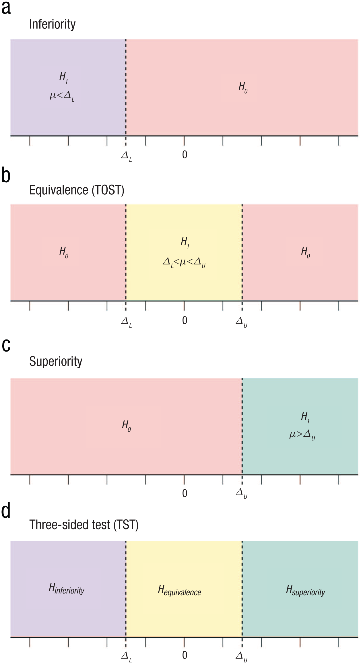
Hypotheses for (constituent tests of) the three-sided testing approach. (a) Inferiority. (b) Equivalence (two one-sided tests [TOST]). (c) Superiority. (d) Three-sided test (TST).
In practice, researchers may often want to test for superiority, inferiority, and equivalence all at the same time. Fortunately, there is a formal procedure that lets one conduct all three tests simultaneously while controlling error rates across all tests, known as three-sided testing (TST). TST is simply a combination of TOST and minimum-effects tests. Initially developed in the field of medical statistics (Goeman et al., 2010), TST is a relevant procedure in a broad range of disciplines, including psychology. In any research project in which analyses include tests for statistical equivalence, TST is a uniform improvement over the more widely adopted TOST procedure. TST permits the same power for equivalence testing as the TOST procedure while simultaneously allowing researchers to test for significant evidence that relationships are bounded outside of their SESOIs, which the TOST procedure alone cannot do. TST thus gives researchers a comprehensive testing framework to assess the practical significance of statistical relationships.
What Is the TST Procedure?
The TST procedure tests three mutually exclusive hypotheses, all of which are related to the same relationship of interest and each of which should lead to a meaningfully different conclusion if accepted: (a)
The TST procedure simply entails running all the tests listed above at once and then using the combined result of all tests to make an overall inference about the practical significance of the effect (see Fig. 2d). For a more technical introduction to TST, see Goeman et al. (2010). In this article, we present an identical formulation of the original TST procedure, combining a TOST procedure, an inferiority test, and a superiority test to make the procedure more easily understandable for researchers who are already familiar with the TOST procedure for equivalence testing. In what follows, we offer two hypothetical examples of psychological-research projects in which TST could be used for effective data-driven decision-making.
Example 1: comparing treatment options for insomnia
Suppose researchers are studying the effects of a new treatment for insomnia. The standard care for individuals suffering from chronic insomnia is sleep-inducing medication combined with cognitive-behavioral therapy for insomnia (CBT-I). However, a new therapeutic approach has been proposed as a substitute for CBT-I: attention and commitment therapy for insomnia (ACT-I).
The researchers would like to know whether it is preferable or even clinically responsible to offer ACT-I instead of standard CBT-I care to insomnia patients. Suppose then that they commission a large-scale randomized controlled trial to study the effectiveness of ACT-I relative to standard insomnia treatment. Insomnia patients in the control group receive the standard course of CBT-I treatment, and patients in the treatment group receive ACT-I instead. The outcome of interest for this trial is the difference in average minutes of sleep per night at endline between patients receiving ACT-I and patients receiving CBT-I. The research team sets an SESOI for this trial based on the number of additional minutes of sleep per night that patients would consider large enough to warrant a change in treatment course. The researchers run a longitudinal survey of patients receiving standard care and find that 15 min per night seems to be the smallest change in sleep duration that patients would consider a large enough benefit to merit changing their course of treatment. This implies that the SESOI for differences in insomnia care is 15 min of sleep per night and that
The researchers develop an official evidence-based policy for the use of ACT-I in insomnia treatment based on TST results:
Inferiority: If ACT-I leads to a reduction of more than 15 min in average nightly sleep duration compared with CBT-I, then therapists will be discouraged from offering ACT-I.
Equivalence: If ACT-I leads to a change in nightly sleep duration within
Superiority: If ACT-I leads to an increase of more than 15 min in average nightly sleep duration compared with CBT-I, then ACT-I will be recommended to replace CBT-I as the standard care offered to insomnia patients.
Inconclusive: If the practical significance of differences between the sleep improvements yielded by ACT-I and CBT-I is inconclusive, then a replication study will be conducted, and results from the two studies will be pooled to provide a conclusive test. If this pooled study still does not yield a precise result, then the mean minutes of sleep gained or lost will be used as a temporary basis for policy until more data become available, and no additional recommendations will yet be made.
Example 2: behavioral research on sales tactics
Consider a set of researchers who are advising a services company. The company sells service packages to clients, offering small, medium, or large packages (increasing in price). Company leadership has noticed that some branches attempt to anchor clients on purchasing the medium package by telling clients that the medium package is the most popular purchase. There is debate among company leadership as to whether this sales tactic is a good idea. Anchoring clients on the medium package will increase sales if this tactic draws clients away from purchasing the small package or no package at all, but will decrease sales if the medium package instead substitutes for the large package, or if the anchoring tactic discourages purchases of any package at all.
Suppose, then, that the company runs an experiment to assess the effects of the anchoring tactic in sales pitches. Company branches are randomly assigned into a treatment group that uses the anchoring tactic and a control group that does not. The company estimates that the cost of coordinating use of a single sales tactic across branches would be $10,000 per month. They therefore decide that any difference in branch-level monthly sales below $10,000 is practically equal to zero and consequently that any difference in such sales exceeding $10,000 is practically meaningful. This implies that the SESOI for this intervention in this company is $10,000 and that
The company’s official stance on the anchoring tactic will depend on the practical significance of the tactic’s impact on sales:
Inferiority: If the tactic leads to a loss in revenue larger than $10,000 per month, then the company will conclude that sales pitches with anchoring are inferior to pitches without anchoring and will ban use of the anchoring tactic in sales pitches across all branches.
Equivalence: If the effect is significantly bounded between −$10,000 and $10,000 per month, then the company will conclude that the tactic’s effect is practically equal to zero and will allow branches to freely choose whether to use the tactic.
Superiority: If the tactic’s effect is significantly greater than $10,000 per month, then the company will conclude that the sales tactic is superior and will mandate its use in sales pitches throughout the company.
Inconclusive: If none of these conclusions can be reached with statistical significance, then the company will delay its decision until more data become available (to ensure error rates are controlled in this case, TST should ideally be combined with a sequential-analysis procedure; see Lakens, 2022).
How to Execute and Interpret TST
In what follows, we start by discussing methods for specifying an SESOI for TST. We then present two identical methods for conducting TST. The methods can be applied to any statistical estimate for which (a) a standard error can be computed and (b) test statistics can be reasonably assumed to be Student
Specifying an SESOI
The first step in TST is to specify a meaningful SESOI. Just as in equivalence testing, specifying an SESOI is the most challenging aspect of TST. In general, how you should proceed with SESOI specification depends very much on the specific question you want to answer and the research field you are working in. No one approach will fit all contexts. To give an impression of the range of SESOI-specification strategies available, we outline four concepts that may be helpful to researchers seeking to define SESOIs in a wide variety of research contexts. In what follows, we focus our recommendations on methods that reduce researcher degrees of freedom whenever possible and highlight methods that are susceptible to “SESOI-hacking.”
Unit interpretability and standardized effect sizes
SESOIs are difficult to specify unless one’s parameter of interest is “unit-interpretable,” that is, unless it is measured in a unit that can be meaningfully reasoned about. For example, the effect of a binary treatment on a dummy variable indicating a depression diagnosis is unit-interpretable because people can easily interpret what it means to switch from control to treatment conditions and can relatively easily interpret what it means for the probability of depression to increase or decrease. Likewise, a regression of annual salary on years of education yields a unit-interpretable parameter because people can easily reason about how many more or fewer dollars per year they will make if they undertake 1 additional year of education.
A common example of a parameter that is not unit-interpretable is a group difference in a Likert scale. Not only does the difference between levels of a Likert scale differ depending on the number of items on the scale and the specific wording of the labels on each item, but also, the meaning of a linear move from one item to the next will conceptually differ depending on the construct measured by the Likert scale.
Whenever possible, it is always preferable to establish SESOIs based on unit-interpretable effect sizes. Unfortunately, most standardized-effect-size measures applied in psychology are not unit-interpretable. Some examples of unit-interpretable standardized-effect-size measures include odds ratios (which are often estimated in biomedical research) and elasticities (which are regularly estimated in economics).
Although standardized effect sizes are often less unit-interpretable than “raw” effect sizes, they nonetheless have unique interpretability properties. Because standardized effect sizes are often used across studies, they make effect sizes comparable across studies. This specific utility of standardized effect sizes was directly referenced in historical American Psychological Association statistical-reporting guidelines, which encouraged the use of effect-size measures that could be easily compared with those of prior studies (Wilkinson & American Psychological Association Task Force on Statistical Inference, 1999).
Standardized mean differences—such as Glass’s (1976)
This distributional approach is far superior to using benchmark values—such as those proposed by Cohen (1988)—to set SESOIs, a practice that methodological guides on equivalence testing and SESOI determination often discourage (see Anvari & Lakens, 2021; Bakker et al., 2019; Funder & Ozer, 2019; Lakens et al., 2018). In many disciplines, there is documented evidence that canonical small effect-size benchmarks are larger than a substantial proportion of published effect sizes (Gignac & Szodorai, 2016; Kraft, 2020; Lovakov & Agadullina, 2021; Paterson et al., 2016). Even SESOIs set using benchmark values based on the distribution of published effect sizes for a given parameter are problematic. Principally, the distribution of published effect sizes is well known to be biased in favor of statistically significant results (Brodeur et al., 2023; Franco et al., 2014; Moniz et al., 2025). This, in turn, results in the inflation of published effect sizes that are considerably larger than those from (robustness) replications (see Brodeur et al., 2024; Camerer et al., 2016, 2018; Gelman & Carlin, 2014; Open Science Collaboration, 2015; Yang et al., 2023). Furthermore, even in a discipline with no publication bias, a published effect size that is practically meaningful in one context may be practically negligible in another; SESOIs for individual studies must be idiosyncratically determined for a specific study’s context. In addition, the large, heterogeneous menu of published estimates typically available to researchers can create avenues for researcher degrees of freedom and opportunities to “hack” the SESOI.
In many contexts relevant to psychological research, one can convert unit-uninterpretable parameters into unit-interpretable parameters by dichotomizing outcomes based on a practically meaningful division. For example, scales used to diagnose mental-health conditions, such as stress or depression, can be dichotomized at thresholds used for clinical diagnosis of those conditions. One practice common in economics is to dichotomize variables using a dummy indicating whether the variable is above or below the median value in the sample. Treatment effects on these dichotomized outcomes are unit-interpretable as effects on diagnosis probability or as effects on the probability of being “above median” on a certain outcome. A key drawback to this approach is that dichotomizing a continuous variable can reduce power by discarding informative variation (Ragland, 1992); so if possible, it is useful for researchers designing new studies to measure constructs in units that render the end parameter that will be estimated in their study unit-interpretable.
Eliciting SESOIs from surveys
Regardless of whether a given parameter is unit-interpretable, the SESOI for that parameter can be reliably established by eliciting judgments on the smallest practically meaningful effect size from independent samples. In psychological research, Anvari and Lakens (2021) termed this an “anchor-based” approach for determining SESOIs. However, anchor-based approaches for SESOI determination actually constitute a broader class of SESOI-determination methods originating in the medical literature, which “anchor” SESOIs to some other estimate (e.g., the medical impact of a major life event or aging a certain number of years; see Lydick & Epstein, 1993). Because such anchor-based methods for setting SESOIs can rely on many possible anchors (see Devji et al., 2020), allowing researchers to select their own anchor creates considerable researcher degrees of freedom and risks of Region of Practical Equivalence (ROPE)-hacking. However, in this broader class of approaches, the SESOI-determination method that Anvari and Lakens identified as anchor-based most closely aligns with methods for determining minimal (clinically) important differences.
Minimal important differences are often elicited from patients or physicians by surveying the smallest effect size that would be large enough to justify changing a course of treatment (Ferreira et al., 2012). For instance, the insomnia-treatment experiment described above uses such a survey to identify the smallest change in sleep that patients would consider clinically meaningful. Outside of the clinical context, Anvari and Lakens (2021) recommended surveying people about the smallest effect size that they would find perceptible. A more generally applicable method in cases in which direct stakeholders are difficult to identify or reach is surveying researchers for their judgments on SESOIs; for a more comprehensive guide on such surveys, see Fitzgerald (2025). Regardless of whether they are elicited from stakeholders or experts, the key component that can make SESOIs elicited from surveys credible is that such SESOIs are determined from a data source that is independent of the research team and their data.
Smallest measurable differences
One potentially useful SESOI is the smallest measurable difference for a given instrument. For example, Brañas-Garza et al. (2021) used equivalence testing to show that the effect of hypothetical stakes on the number of risky choices made on a multiple-price list is bounded beneath one risky choice. The SESOI could also be set to 1 for a single Likert item or the number of correct answers on a test because this is similarly equivalent to the smallest measurable difference in those outcomes. In cases in which such measures are present on both sides of a regression equation, the commensurate smallest measurable difference would be equivalent to a 1-point increase in the independent variable being associated with a 1-point change in the dependent variable (i.e., a regression coefficient of
A 1-point shift in a composite Likert scale—that is, a scale composed using a (weighted) average—is not the same as the smallest measurable difference for that scale and should not be interpreted as one. Consider the widely used nine-item Patient Health Questionnaire (PHQ-9) for depression diagnosis, which is composed of 4-point Likert items (Kroenke et al., 2001). The PHQ-9 scale is often reported as a raw sum of points across its nine items, ranging from 0 to 27. At this unit scale, a 1-point difference is the smallest measurable difference in the PHQ-9. However, the PHQ-9 could in principle be converted into a composite scale by dividing this sum total by 9, effectively creating an average score per item; many Likert scales are transformed in this way in psychological research. It would be inappropriate to interpret a 1-point difference in this composite scale as the smallest measurable difference for the PHQ-9. Consider that Kroenke et al. (2001) found that the raw PHQ-9’s raw standard deviation is 6.1 in patients with major depressive disorder. This implies that a 1-point difference in a composite PHQ-9 scale would exceed two-thirds of a standard deviation, whereas a 1-point difference in the raw scale would be just over 0.16 SD.
Cost–benefit analysis
In applied settings in which effects can be tied to specific costs and benefits—for example, when a certain intervention has a known cost and unit-interpretable benefits have a distinct financial valuation—it may be possible to specify SESOIs based on cost–benefit analysis. For example, the sales-tactic experiment described above uses a cost–benefit analysis to set the SESOI. When the SESOI is set in this way, one can explicitly test whether a given observed effect is large enough for intervention benefits to outweigh costs. See Fitzgerald (2025) for more detailed guidance on practical significance testing with SESOIs determined through cost-benefit analysis.
TST using one-sided tests
The first way to conduct TST is by obtaining
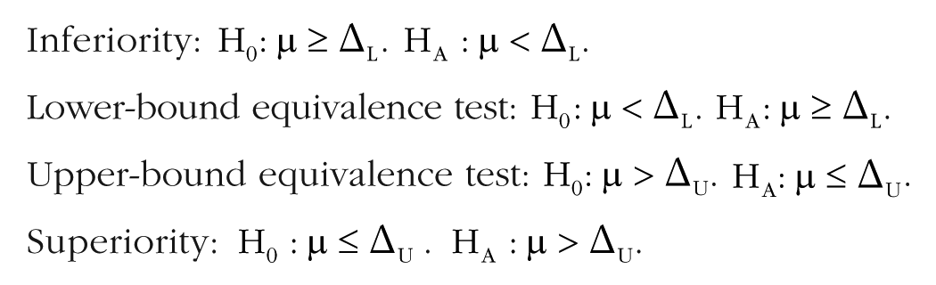
Inferiority:
Lower-bound equivalence test:
Upper-bound equivalence test:
Superiority:
Running these four tests will yield four one-sided
Practically significant and negative: If the one-sided inferiority-test statistic is significant at level
Practically equal to zero: If both of the two one-sided tests for equivalence are significant at level
Practically significant and positive: If the one-sided superiority-test statistic is significant at level
Inconclusive: If none of the above conditions hold, then remain uncertain about the practical significance of the relationship.
Notice that even though we have set a significance level of 5%, the
No multiple-hypothesis-testing corrections are required for the lower- and upper-bound equivalence tests because the TOST procedure already requires that both one-sided tests are significant at level
TST using confidence intervals
An identical procedure for conducting TST is to compute two confidence intervals (CIs) for the relationship of interest—one at
To start, compute the
Practically significant and negative: If the
Practically equal to zero: If the
Practically significant and positive: If the
Inconclusive: If none of the above conditions hold, then remain uncertain about the practical significance of the relationship.
Figure 3 illustrates this CI procedure for a significance level of
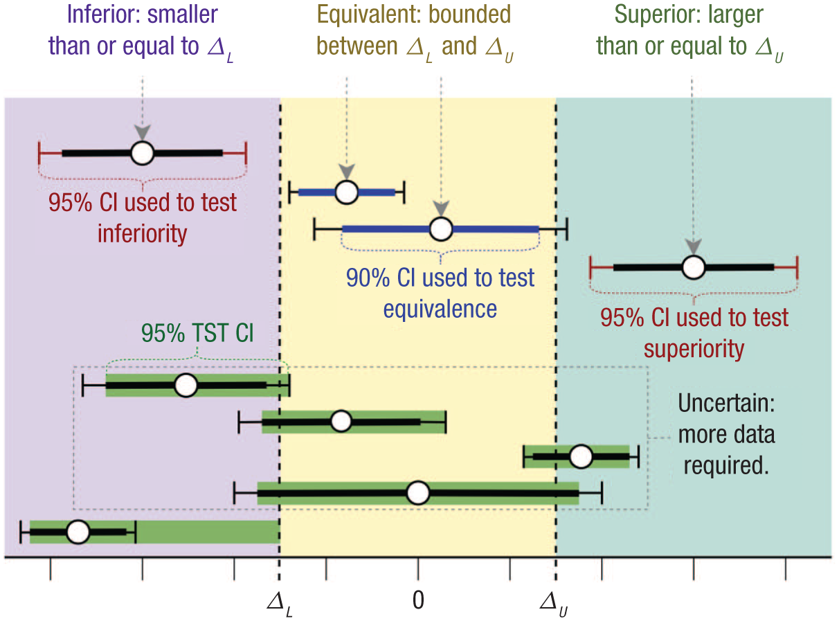
Illustration of how different test results should be interpreted in three-sided testing (TST) at a significance level of
The TST CI
Although the
and its upper bound can be written as

Figure 3 displays the
Note that the regions rejected by the TST CI yield the same practical-significance conclusions as the decision rule discussed in TST Using CIs, the latter of which is much simpler to interpret. The TST CI does not in any way change conclusions arising from the TST procedure discussed in TST Using CIs and TST Using One-Sided Tests but, rather, constrains the precision that can be reliably reported for the estimate when TST is implemented. Intuitively, this is because TST induces a power trade-off: Although TST provides researchers with more power to reach statistical-significance conclusions across multiple tests, this comes at the cost of reducing the precision with which researchers can bound the relationship of interest if it significantly exceeds the SESOI bounds.
In the software applications described below, both classic and TST CIs are computed automatically for convenience. When reporting TST results, we recommend displaying triple-banded CIs displaying the
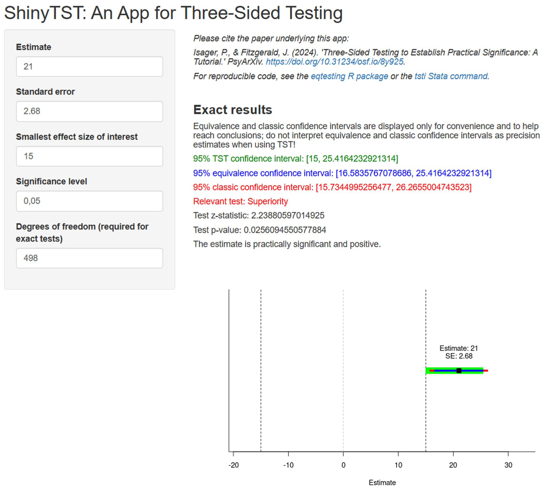
ShinyTST example for an estimate of 21, standard error of 2.68, and smallest effect size of interest of 15.

ShinyTST example for an estimate of 10, standard error of 2.68, and smallest effect size of interest of 15.

ShinyTST example for an estimate of −20, standard error of 2.68, and smallest effect size of interest of 15.

ShinyTST example for an estimate of −12, standard error of 2.68, and smallest effect size of interest of 15.

A partitioning of the parameter space permitting a combination of three-sided testing (TST) and standard null hypothesis significance testing. Estimates are displayed along with
TST using the ShinyTST application
To enable as many readers as possible to apply TST in their own data analyses, we have developed a stand-alone, point-and-click application. The ShinyTST app requires four inputs and has one optional input. Required inputs include an estimate (e.g., a mean difference or a correlation coefficient), the standard error of that estimate, the SESOI (in the same units as the estimate), and the significance level
Consider again our hypothetical experiment on treatment options for insomnia. Based on differences in hours slept per night in each treatment condition, we want to decide if the novel ACT-I is practically inferior, equivalent, or superior to standard CBT-I treatment. We can conduct TST in the ShinyTST app to help us make this decision.
Example 1: a practically significant relationship
Suppose that in our experiment we observe that compared with the control group receiving CBT-I, patients treated with ACT-I sleep 21 more min per night at endline, with a standard error of 2.68 min. Our significance level is 5%, and as discussed in Example 1: Comparing Treatment Options for Insomnia, our SESOI is 15 min of sleep per night. We have 500 participants in our experiment, implying that our tests are conducted with 498 degrees of freedom.
Figure 4 displays where to input these parameters in ShinyTST and the resulting output. Following the TST procedure, we would conclude that this relationship is superior to our SESOI. The “Relevant test” output tells us that the relevant test to look at in this case is the superiority test because the observed estimate is more positive than the upper SESOI bound. The color of the “Relevant test” output signals which classic CI is relevant for drawing a conclusion. In this case, the red-colored 95% classic CI is the relevant one, and we can see in both the numeric output and the accompanying graph that the lower 95% classic CI bound is greater than the upper SESOI bound of 15 min of nighttime sleep. That is, the entire 95% classic CI falls above the SESOI. Accordingly, the test
Example 2: a relationship practically equal to zero
Now suppose instead that patients receiving ACT-I sleep 10 min more than the control group, keeping everything else the same as before. The estimate is smaller than the SESOI, but is it precise enough that we can confidently rule out practically meaningful differences in sleep between treatments? Figure 5 displays the TST results for this estimate.
In this case, we would conclude that the relationship is practically equal to zero. That is, the difference in average sleep times between ACT-I and CBT-I patients is significantly bounded within
Example 3: inconclusive results
Now suppose we observe that at endline, patients receiving ACT-I sleep an average of 20 min less per night than patients receiving CBT-I, again holding all else constant. This estimate is more negative than our lower SESOI bound, but is it estimated precisely enough that we should conclude that ACT-I is a clinically irresponsible treatment? Figure 6 displays the TST results for this estimate.
In this case, we arrive at an inconclusive result. As in Figure 4, the “Relevant test” output indicates that the red-colored 95% classic CI is relevant for this estimate because the estimate is more negative than the lower SESOI bound. The
Finally, suppose instead that ACT-I patients sleep 12 min less per night than CBT-I patients on average, again holding all else constant. As in Example 2, this estimate is smaller in magnitude than the SESOI. But is it precisely bounded enough that we should give clinicians free reign to select between ACT-I and CBT-I at will? Figure 7 displays TST results for this estimate.
This case also yields an inconclusive result. As in Figure 5, the “Relevant test” output indicates that the blue-colored 90% classic CI is relevant for this estimate because the estimate is between the SESOI bounds. This estimate’s 90% classic CI intersects one of the SESOI bounds, and the TST
TST in R, Jamovi, and Stata
Although our point-and-click application is easy to use, statistical software is better for reproducible analyses. We therefore supplement the ShinyTST app and the tutorials in this article with examples of how to conduct TST in both R and Jamovi. These examples work with data from a case similar to that discussed in Example 1: A Practically Significant Relationship and, respectively, use the tst command in the eqtesting R package (Fitzgerald, 2025) and the TOSTER module in Jamovi (Caldwell, 2022; Lakens, 2017). We direct readers more familiar with Stata to the tsti command, which can be downloaded from Statistical Software Components.
Supplementary material SM1 (https://osf.io/6wbxh) demonstrates how to conduct TST in R using either four one-sided tests or CIs. In addition, the tutorial demonstrates how to conduct TST using the tst function in the eqtesting R package (Fitzgerald, 2025). The tst function is an R-based version of the ShinyTST app. Finally, the tutorial demonstrates how to adapt the tst function to your own data and how to retrieve the statistics used as input to tst from various statistical models in R.
Supplementary material SM2 (https://osf.io/ncxvg) provides a Jamovi file that contains the same simulated data as the R script and a TST analysis conducted using Jamovi’s TOSTER module. In the Jamovi file, the “Results” pane contains two identical TOST independent sample
Reporting TST Results
When reporting TST results, include the following information:
The relevant test (inferiority, equivalence, or superiority): This information is automatically provided by the ShinyTST app, the tst command in R, and the tsti command in Stata, but this can also be inferred directly by examining the point estimate’s relationship with the SESOI bounds.
The TST
The standard error and
The conclusion of the test: Interpret whether the relationship is practically significant and negative, practically equivalent to zero, or practically significant and positive, or whether the TST results are inconclusive. TST regions rejected by the TST CI can also be rejected.
In addition to visualizing triple-banded CIs of the form in Figures 4 to 7, the superior TST results in Example 1: A Practically Significant Relationship could be reported as follows:
We conducted a three-sided test to assess whether ACT-I leads to at least 15 min more sleep per night than standard CBT-I care, which is the SESOI in this setting. Our experimental results imply that ACT-I yields significantly more than 15 min extra sleep on average compared with CBT-I (
The practically negligible result in Example 2: A Relationship Practically Equal to Zero could instead be reported as follows:
Our experimental results imply that differences in average nighttime sleep between patients treated with ACT-I and patients treated with CBT-I is significantly smaller than 15 min per night (
The uncertain result reported first in Example 3: Inconclusive Results could be reported as follows:
Given our experimental results, the practical significance of sleep differences between ACT-I and CBT-I is inconclusive (
Power Analysis and Sample-Size Planning for TST
Best practices for computing necessary sample sizes for sufficient power in TST differ from those for computing power and sample sizes for equivalence testing or minimum-effect testing. Unlike these tests, the TST procedure tests several hypotheses at once. Consequently, having sufficient a priori power for conclusive TST results requires having sufficient power for all tests. Our recommendations for computing sample sizes for sufficient power thus differ depending on whether you expect to obtain an estimate larger or smaller in magnitude than the SESOI.
Appendix A in the Supplemental Material provides interested readers with a comprehensive guide on power analysis for TST. As in other power analyses, this requires researchers to have an informative a priori expectation of both the effect size they will observe and the standard deviation(s) of their outcome(s) of interest. Both quantities can be derived from either pilot studies or the results of similar previous studies. Standard deviations may also potentially be set using normative data on population-level variation in outcomes of interest; for an example, see Example 1: Statistical and Inferential Power for a Large Effect.
TST has more inferential power than both standard NHST and TOST. That is, researchers can reach more informative conclusions with TST than they can with standard NHST and TOST while simultaneously controlling error rates for these conclusions. The price one has to pay for this improved inferential power is lower statistical power to declare “significant” effects compared with standard NHST. To illustrate this, consider the following two examples.
Example 1: statistical and inferential power for a large effect
Returning to our insomnia treatment experiment from Example 1: Comparing Treatment Options for Insomnia, suppose that we expect that the difference in average nighttime sleep between ACT-I patients and CBT-I patients will be 30 min per night, double the SESOI. We expect from population-level data that nighttime sleep varies with a standard deviation of 65 min per night (Sivertsen et al., 2020). To calculate the required sample size for a superiority test in R, use the base power.t.test function with the delta parameter set to the difference between the effect size you want to power to and the upper SESOI bound: sesoi = 15 effect = 30 stdev = 65 power.t.test( delta = effect - sesoi, sd = stdev, sig.level = 0.05, power = 0.80, type = ‘two.sample’, alternative = ‘two.sided’)
To have at least 80% power to detect a sleep effect of 30 min per night with an SESOI of 15 min per night, we would need 148 people in each group. Compare this with statistical power under standard NHST, in which our goal is simply to test whether the effect is different from zero: effect = 30 stdev = 65 power.t.test( delta = effect, sd = stdev, sig.level = 0.05, power = 0.80, type = ‘two.sample’, alternative = ‘two.sided’)
For 80% power to detect this effect under standard NHST, we need only 37 people in each group. The larger the SESOI bounds are, the more underpowered TST is to detect “significant” effects relative to standard NHST (conditional on the SESOI being less than the anticipated effect size; superiority and inferiority tests naturally have zero power when the SESOI exceeds the anticipated effect size). However, with standard NHST, we can conclude only that the effect is larger than zero; we cannot formally conclude anything about the practical significance of the effect. In contrast, TST allows us to formally draw a conclusion about practical significance. Therefore, compared with standard NHST, TST sacrifices statistical power to achieve greater inferential power.
Note that here, the TOST procedure has zero statistical power because the effect size is presumed to fall outside of the SESOI bounds. The TOST procedure never yields statistically significant results for effect sizes larger than the SESOI; so in this example, TST yields no additional gains in inferential power to conclude that effects are practically negligible (although this is not a loss relative to standard NHST because standard NHST also does not allow researchers to formally test this conclusion). In what follows, we provide an example in which TST does yield additional inferential power in this way.
Example 2: statistical and inferential power for a practically negligible effect
Suppose instead that we expect no differences in nighttime sleep between ACT-I and CBT-I patients (keeping everything else the same as before). In this example, we expect to observe an effect bounded within the SESOI bounds. To calculate the required sample size for an equivalence test in R, we use the power_t_TOST function in the TOSTER package (see Lakens & Caldwell, 2025): library(TOSTER) sesoi = 15 effect = 0 stdev = 65 power_t_TOST( delta = effect, sd = stdev, eqb = sesoi, alpha = 0.05, power = 0.80, type = ‘two.sample’)
Given an SESOI of 15 min of nighttime sleep, to have at least 80% power to conclude that an observed difference in average sleep times of 0 min per night is practically equivalent to 0 under TST, we would need 162 people in each group. Note that this is exactly identical to the number of people we would need to conclude that such a relationship is practically negligible under standard equivalence testing. The equivalence-test component of TST is identical to the TOST procedure, so statistical power to conclude that an effect is practically negligible is also identical between TST and the TOST procedure. This is why we say that TST is a uniform improvement over the TOST procedure. It has the same statistical power as the TOST procedure, but it has increased inferential power because TST can also reach conclusions about practically meaningful effects through inferiority and superiority tests, which the TOST procedure alone cannot.
Note also that standard NHST has neither statistical nor inferential power when the true relationship is zero. Standard NHST cannot reach the correct conclusion when there is no relationship, which is why many researchers turn to equivalence testing in the first place. TST has greater inferential power than standard NHST for both null and nonzero relationships.
TST in Complex Statistical Designs
The examples above and in the supplementary files all demonstrate how to conduct TST for relatively simple models such as
When conducting exploratory analyses in large data sets with many variables, one should keep in mind that TST requires correction for multiple comparisons in just the same way that standard NHST does. When testing one single relationship, there is no need to correct for multiple-hypothesis testing across the superiority, inferiority, and equivalence tests in TST because the size of the union of these tests is controlled at nominal levels (provided that one employs the significance thresholds discussed in TST Using One-Sided Tests and TST Using Confidence Intervals). However, across tests of multiple relationships, each execution of TST is independent, and correction for multiple comparisons across the TST executions is therefore required.
Combining TST With NHST
If we expect the SESOI to change in the future, then it may be worth combining TST with standard NHST. Returning to our experiment on anchoring sales tactics in Example 2: Behavioral Research on Sales Tactics, the company’s SESOI for branch-level sales may increase over time as the company grows in size. Likewise, the smallest practically meaningful change in branch-level sales may decline in periods when the company experiences financial distress. It thus may be useful to record whether the anchoring tactic has some nonzero effect on sales to inform future experiments and policies.
To combine TST and standard NHST, simply add a two-sided test against zero to the TST procedure outlined in this article. Figure 8 shows how this alteration augments the TST procedure. This effectively partitions the
Conclusion
Whenever researchers can specify a meaningful SESOI, TST is a superior testing procedure compared with both standard NHST and TOST procedures. TST allows one to detect significant evidence that a relationship is practically significant or practically negligible and to test more meaningful predictions than standard NHST (see also Lakens, 2022; Meehl, 1967). Researchers should therefore strongly consider TST as their default frequentist test procedure if they can specify a meaningful SESOI.
Researchers conducting quantitative analyses virtually always wish to make concrete statements about whether their estimates “matter.” Researchers have historically done this by leaning on the precision guarantees offered by standard NHST, labeling estimates that can be precisely bounded away from zero as “statistically significant.” However, this practice somewhat abuses the definition of the word “significant” and conflates estimates’ practical significance with their precision. This conflation between precision and practical significance means that null estimates become conflated with imprecise estimates, which is a key motivation behind publication bias against null results (Fitzgerald, 2025).
TST addresses this by separating estimates’ precision from their significance. In TST, the significance of estimates is determined by their relationship with the SESOI, and the precision of the estimate is judged by the formal hypothesis tests in the TST framework. In so doing, TST allows researchers to more credibly distinguish which estimates are practically meaningful and which ones are practically negligible.
Footnotes
Acknowledgements
We thank Jelle Goeman for helpful comments and feedback. All errors are our own. The anchoring-tactic example in this article was first suggested by ChatGPT.
Transparency
Action Editor: David A. Sbarra
Editor: David A. Sbarra
Author Contributions