
Abstract
Psychologists are often interested in whether an independent variable has a different effect in condition A than in condition B. To test such a question, one needs to directly compare the effect of that variable in the two conditions (i.e., test the interaction). Yet many researchers tend to stop when they find a significant test in one condition and a nonsignificant test in the other condition, deeming this as sufficient evidence for a difference between the two conditions. In this Tutorial, we aim to raise awareness of this inferential mistake when Bayes factors are used with conventional cutoffs to draw conclusions. For instance, some researchers might falsely conclude that there must be good-enough evidence for the interaction if they find good-enough Bayesian evidence for the alternative hypothesis, H1, in condition A and good-enough Bayesian evidence for the null hypothesis, H0, in condition B. The case study we introduce highlights that ignoring the test of the interaction can lead to unjustified conclusions and demonstrates that the principle that any assertion about the existence of an interaction necessitates the direct comparison of the conditions is as true for Bayesian as it is for frequentist statistics. We provide an R script of the analyses of the case study and a Shiny app that can be used with a 2 × 2 design to develop intuitions on this issue, and we introduce a rule of thumb with which one can estimate the sample size one might need to have a well-powered design.
“This independent variable had a statistically significant effect in condition A, and by contrast, we found no statistically significant effect in condition B.” Many researchers believe that these findings are sufficient to support the claim that there is a difference between conditions A and B in the effect of the variable. However, such an inference does not follow from these results, as it requires the test of the difference in the effect between the conditions, or, in other words, the test of the interaction (Abelson, 1995, p. 111; Gelman & Stern, 2006). This inferential mistake is common in neuroscience (Nieuwenhuis, Forstmann, & Wagenmakers, 2011), and one can safely assume that psychologists are also not immune from committing it. Although this mistake is now well recognized when it comes to null-hypothesis significance testing, how does it relate to the use of Bayes factors?
When conventional cutoffs are used for Bayes factors (see Box 1 for a brief introduction on the interpretation of Bayes factors via the conventional cutoffs), there may be conditions in which this inferential mistake is even more likely than with frequentist statistics. If there is good-enough Bayesian evidence for the alternative hypothesis, H1, in one condition and for the null hypothesis, H0, in another, surely one can conclude that the effect is bigger in the first condition than the second! Through personal discussions with colleagues, we have gotten the impression that it may not be obvious for many researchers that this latter conclusion is incorrect even if they are aware of the corresponding inferential mistake when it comes to frequentist statistics. Readers can explore the extent to which they are attracted toward this inappropriate conclusion, which asserts an interaction in the absence of a direct test of it, by considering the hypothetical study described in Box 2 (a scenario that we discuss in detail as Example 2 later in this Tutorial). As they read the information in the box, they can also test whether they would be more inclined to accept this inappropriate conclusion when it is based on frequentist or on Bayesian statistics.
The Interpretation of the Bayes Factor
The Bayes factor is a continuous measure of the strength of relative evidence for two hypotheses according to their ability to predict the data at hand (Dienes, 2016; Kruschke & Liddell, 2018; Rouder, Speckman, Sun, Morey, & Iverson, 2009). In this Tutorial, we report Bayes factors that represent the evidence for the alternative hypothesis, H1, over the null hypothesis, H0. A Bayes factor of 1 means that the two hypotheses can predict the data equally well. The convention we follow (which is not universal) is that the larger the Bayes factor, the better H1 fits the data compared with H0, and the smaller the Bayes factor, the better H0 fits the data compared with H1. To aid decision making, Jeffreys (1961) suggested BF > 3 as the cutoff of substantial evidence for H1 over H0. Note that Jeffreys chose this value with the intention that Bayes factors should lead to judgments similar to those that follow from null-hypothesis significance testing; that is, a statistical test resulting in p = .05, the usual cutoff for rejecting H0, will usually provide a Bayes factor around 3 as long as the obtained effect size is about what was predicted. Following a principle of symmetry, we interpret BF < 1/3 as substantial evidence for H0 over H1. However, we do not mean to indicate that BF > 3 should be automatically accepted as the level of good-enough evidence for H1 over H0. Indeed, it is a rough guideline, and the level of good-enough evidence remains a matter of scientific debate (e.g., currently, the level of good-enough evidence for H1 is defined as BF > 6 at Cortex and as BF > 10 for Registered Reports at Nature Human Behavior). Nonetheless, in this Tutorial, we apply the cutoff of substantial evidence as the cutoff for good-enough evidence.
Test Your Intuitions
At a Golf Club in Sussex, a coach stumbled upon a sport psychology article concluding that mental training (e.g., imagining hitting the ball with a golf club) can help golfers improve their skills when it is combined with real training. Before implementing the mental training in all student groups, the coach decided to test whether players can benefit from it. Therefore, the coach asked the students in one group to engage in mental training (on top of the traditional training) twice every week for the next 3 months. The coach also had a control group in which the students underwent traditional training but were not told to do the mental training; the students in this group had skills roughly identical to those of the students in the mental-training group. The coach assessed the performance of the students at baseline and after 3 months of training. The evaluation was performed on an interval scale from 0 to 10. Given the results of past studies with other sports, the coach expected that after 3 months of training, performance could improve by about 2 units.
To draw conclusions from the analyses, the coach used null-hypothesis significance testing, and the alpha level was set at the traditional .05. The coach reported the results of two statistical tests and a conclusion based on those tests. Evaluate the appropriateness of the following conclusion on a scale from 0 (you feel that the conclusion is completely inappropriate) to 10 (you feel that the conclusion is completely appropriate based on the information at your disposal): Comparing baseline and posttraining performance in the control group yielded a nonsignificant result, t(19) = 0.29, mean difference = 0.11, p = .776. However, in the group of students who engaged in the mental training, there was a significant improvement in performance after 3 months, t(19) = 2.61, mean difference = 0.81, p = .017. On the basis of these results, the coach concluded that traditional training is more efficient when it is combined with mental training than when it is not.
Now suppose that the coach used Bayes factors (see Box 1), instead of null-hypothesis significance testing, to draw conclusions. Given that the coach had reasons to expect an effect of about 2 units, he used a half-normal distribution with a standard deviation of 2 as the model for the alternative hypothesis. Assess the appropriateness of the following conclusion based on the Bayes factors by choosing a value from the same scale of appropriateness (i.e., 0 means that you feel that the conclusion is completely inappropriate, and 10 means that you feel that the conclusion is completely appropriate): Comparing baseline and posttraining performance of the control group yielded good-enough evidence for the null hypothesis of no change, t(19) = 0.29, mean difference = 0.11, p = .776, BFH(0, 2) = 0.24 (see the main text for an explanation of the notation for Bayes factors). However, the analysis of the data of the mental-training group yielded good-enough evidence supporting an improvement in performance after 3 months of training, t(19) = 2.61, mean difference = 0.81, p = .017, BFH(0, 2) = 6.12. On the basis of these results, the coach concluded that traditional training is more efficient when it is combined with mental training than when it is not.
The central goal of this Tutorial is to substantiate in readers the statistical intuition that to claim the existence of a difference in the effect of an independent variable between two conditions or groups, one always needs to test the interaction, and that this principle is as true for Bayesian as for frequentist statistics. We present a hypothetical case study in which Bayes factors for evidence of the presence of an effect are calculated for an experimental group and a control group for which frequentist statistical tests were significant and non-significant, respectively. By this approach, we aim to illustrate that there are cases in which using Bayes factors instead of frequentist statistics could make it more likely to commit the inferential mistake that is the focus of this Tutorial, and there are cases in which it may be the other way around. By increasing the sample size and reducing the raw effect size in our case study, we cover all the scenarios in such a case: insensitive evidence versus evidence for an effect coupled with an insensitive test of the interaction, insensitive evidence versus evidence for an effect coupled with a sensitive test of the interaction, evidence for no effect versus evidence for an effect coupled with an insensitive test of the interaction, and evidence for no effect versus evidence for an effect coupled with a sensitive test of the interaction.
The Case Study
Consider the hypothetical study, described in Box 2, in which a golf coach is trying to test whether or not adding mental training to traditional training can improve golf performance. To investigate this question, the coach randomly assigned students to a group that received traditional training only (henceforth, the control group) and a group that received traditional plus mental training (henceforth, the mental-training group). The coach assessed golf performance at baseline and after 3 month of training. Therefore, the study had a 2 × 2 mixed design. Hence, the crucial test of the idea that one can benefit more from golf training if it is combined with mental training boils down to a test of the 2 × 2 interaction of time of assessment (baseline vs. posttraining) and type of training (traditional vs. traditional plus mental). For the sake of simplicity, imagine that golf performance was measured on a scale from 0 to 10, and the coach expected that the mental training should improve performance by about 2 units.
Justifying the Model of H1 and the Model of the Data
To compute a Bayes factor, one needs to specify the parameters of the models representing the predictions of the hypotheses under comparison (see Box 3 for more information on the essential model choices that must be made when calculating a Bayes factor). The model of H0 assumes no difference in the population. To model the prediction of H1 in our case study, we employed a half-normal distribution with a mode of zero. The properties of the normal distribution align with the scientific intuition that small effect sizes are more probable than large ones (Dienes & Mclatchie, 2018), and we opted for a half-normal distribution because it is in line with the directional prediction of H1. To specify the standard deviation of the distribution, we applied the expectation of the hypothetical coach, who assumed that performance should improve by about 2 units. 1 In addition, we needed a model of the data (also referred to as likelihood; see Box 3). We used the t distribution, which is recommended over the normal distribution when the variance of the data is estimated because it is unknown (Dienes & Mclatchie, 2018). To notate the Bayes factors in our case study, we use BFH(0, 2), following the convention introduced by Dienes (2014). This notation includes all the necessary information about the model of H1: The subscript “H” indicates a half-normal distribution, “0” refers to the mode, and “2” refers to the standard deviation of the distribution. All Bayes factors reported in this Tutorial represent evidence for H1 over H0.
The Anatomy of the Bayes Factor
In order to assess the predictive ability of hypotheses, one needs to create models that represent their predictions. Modeling the prediction of no difference (the null hypothesis) is the straightforward part of the process. However, specifying the predictions of the alternative hypothesis requires scientifically informed decisions in every case, and so it can be a subject of debate. For instance, one needs to define the shape and parameters of the distribution representing the predictions of the alternative hypothesis as a function of the possible population effect sizes. Should the distribution be a uniform, t, or normal distribution, and should it be one-tailed or two-tailed? Should the distribution be centered on zero or on a nonzero population value? What should be the level of variance in the model? The discussion of these decisions is beyond the scope of the current Tutorial, so we refer readers to Dienes (2015, 2019) and Dienes and Mclatchie (2018). Nonetheless, we justify all of the choices about the model specifications in our case study. Finally, in specifying the alternative hypothesis, one needs to define the likelihood function, which models the probability of the data given different population effect sizes.
Specifying all of these parameters requires the researcher to make many decisions, which has the side effect of increasing analytic flexibility and so the opportunity to cherry-pick the results supporting the researcher’s pet theory. The most crucial step during which one can introduce bias is perhaps the model specification of H1, which, in some cases, can have a drastic effect on conclusions. One way to reduce bias is by constraining analytic flexibility through preregistering the exact parameters of the model of H1 or the strategy with which one will acquire those parameters (Chambers, 2013; Munafò et al., 2017). One can also consider reporting a robustness region that indicates the range of parameters (e.g., standard deviations of the half-normal distribution modeling H1) that would lead to the same conclusion (i.e., good-enough support for H1 over H0, insensitive evidence, good-enough support for H0 over H1) as the chosen model specification (Dienes, 2019). Robustness regions can diminish bias by increasing transparency regarding the analytic choices, much as multiverse analyses do (Steegen, Tuerlinckx, Gelman, & Vanpaemel, 2016). Robustness regions have the additional benefit that when there are good rationales for a variety of model specifications, one can ascertain the robustness of one’s chosen model specification by simply checking whether all plausible parameters lie within the robustness region. In this Tutorial, we report the robustness region for every Bayes factor in the following format: RRconclusion[min, max], where “min” indicates the smallest and “max” indicates the largest standard deviation of the model of H1 that leads to the same conclusion. We indicate the original conclusion in the subscript of the robustness region by reporting one of the following: BF < 3, 1/3 < BF < 3, or BF > 3.
Disclosures
All the materials of this Tutorial are available on the Open Science Framework, at https://osf.io/jbuv7. These materials include the R script of the Bayes factor analyses introduced here and the script of the Bayes factor function. They also include the R script of a simple and interactive Web application, a Shiny app, that can calculate the Bayes factors of 2 × 2 between-groups and within-participants designs. Box 4 presents an example of the usage of the Bayes factor R script (namely, the test of the interaction in the example we discuss next), and Figure 1 portrays how the Shiny app can be applied to compute all three Bayes factors of this example. The Bayes factor Shiny app can be accessed at https://bencepalfi.shinyapps.io/Bayesian_Interaction_App/.
Calculating the Bayes Factor in R
To calculate the Bayes factor in R, one needs to obtain the summary statistics of the data (mean, standard error, and degrees of freedom) and decide on the parameters of the model of the alternative hypothesis, H1.
The following R script reproduces the results of the test of the interaction in Example 1 (the # symbol identifies comments that are included to help readers and will be ignored by R when the script is run):
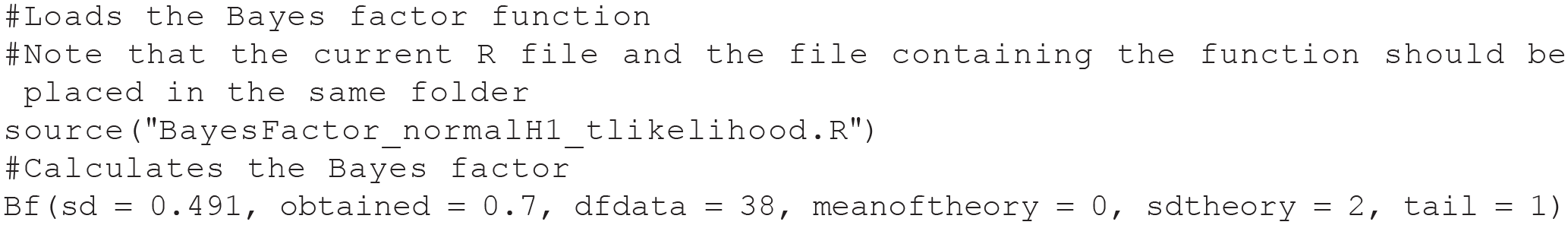
The first three arguments of the function specify the parameters of the likelihood function: the standard error, the estimate (i.e., raw effect size), and the degrees of freedom of the distribution, respectively. The last three arguments define the parameters of the model of H1: the center (or mode in the case of a one-tailed distribution) and the standard error of the distribution and whether it is one- or two-tailed. When all parameters are provided, the function returns a vector containing the value of the Bayes factor (evidence for H1 over the null hypothesis).
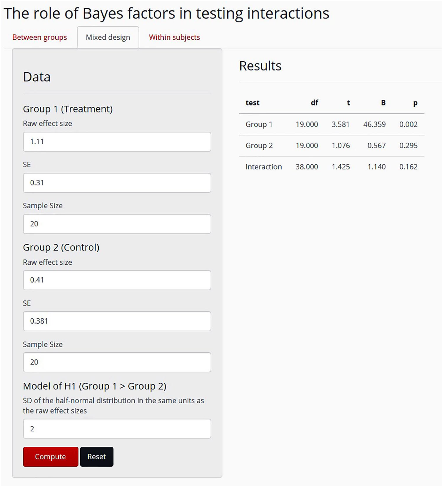
Print screen of the Shiny app at https://bencepalfi.shinyapps.io/Bayesian_Interaction_App/. For 2 × 2 designs, this app calculates the Bayes factor separately for each of the two groups and for the interaction, given the following statistical parameters: the raw effect size and its standard error for each group, the sample size, and the standard deviation of the half-normal distribution that models the predictions of the alternative hypothesis, H1. In the top left corner of the screen, the user can select from the “Between groups,” “Mixed design,” and “Within subjects” options. The between-groups and mixed-design options are identical in that they run an independent-samples t test to test the interaction, and they request the same input parameters. For the within-subjects design, the user needs to provide the raw difference between the conditions and its standard deviation in addition to the parameters needed for between-groups and mixed designs. The results appear on the right side of the screen, once the “Compute” button is pressed. The Shiny app reports the degrees of freedom, the t value, the Bayes factor (“B”), and the p value for each group (or condition) and for the interaction between the independent variables. The data and results shown here are for Example 1 in the text.
Example 1: When the Bayes Factor Helps the Researcher Avoid Committing the Inferential Mistake
In our hypothetical study, suppose that the coach found that the test comparing baseline and posttraining performance was significant in the mental-training group, t(19) = 3.58, mean difference = 1.11, p = .002, and was not significant in the control group, t(19) = 1.08, mean difference = 0.41, p = .295. Given these results, the coach concluded that the effect of traditional training is expressed (at least after 3 months of training) only if it is combined with mental training. This conclusion would be premature for two reasons. First, one cannot claim the absence of an effect on the basis of a nonsignificant test (Cohen, 1994; Dienes, 2014; Rouder, Speckman, Sun, Morey, & Iverson, 2009), and so it is false to imply that there is evidence against the effectiveness of the training in the control group. There is no evidence for the contrary either. The coach simply needs to refrain from making a decision. Second, a more relevant point for the purpose of the current Tutorial is that the dissimilarity of two categorical statements (i.e., significant improvement vs. not significant improvement) does not allow a meaningful categorical statement about the difference between the two groups (i.e., the difference is not necessarily significant in itself; Abelson, 1995, p. 111). From this second point, it follows that one needs to test the difference directly to make any meaningful claim about the interaction between time of assessment and group. The test of the interaction, however, yields a nonsignificant result, t(38) = 1.43, mean difference = 0.70, p = .162, which means that one needs to suspend judgment regarding the influence of the mental training on the effectiveness of traditional golf training.
The question arises, what conclusions would one draw in this scenario if one relied on Bayes factors? These data translate into substantial evidence for the effectiveness of the training in the mental-training group, BFH(0, 2) = 46.36, RRBF > 3[0.2, 36.3], and insensitive evidence for the effectiveness of the training in the control group, BFH(0, 2) = 0.57, RR1/3 < BF < 3[0, 3.5], as well as for the interaction directly comparing the effectiveness of the training in the two groups, BFH(0, 2) = 1.14. RR1/3 < BF < 3[0, 7.4]. Clearly, one cannot easily claim that good-enough evidence for the effect of training in one group and insensitive evidence for the effect of training in the other group is good-enough evidence in itself for a difference between the groups. Apparently, using Bayes factors may help one avoid the inferential mistake regarding the interaction even if one were to ignore the results of the direct test of the interaction.
The only way to come to a conclusion regarding whether or not mental training combined with traditional training is superior to traditional training alone is to collect more data until one obtains evidence in one direction or the other. Optional stopping is not a problem for Bayesian statistics; the Bayes factor will retain its meaning regardless of the stopping rule applied (Dienes, 2016; Rouder, 2014 2 ). Thus, one can check the Bayes factor every time one recruits a new participant and stop once the Bayes factor reaches a good-enough level of evidence. For example, in this scenario, assuming that the raw effect sizes and their variances remain constant, the coach would need to recruit 94 participants in total (47 per group) to have substantial evidence for the interaction, BFH(0, 2) = 3.09, RRBF > 3[0.3, 2.0]. In this scenario, the evidence for the efficacy of the training in the control group would still be insensitive, BFH(0, 2) = 0.89, RR1/3 < BF < 3[0, 5.4]. Thus, there can still be evidence for a difference in effects between two groups when there is evidence for an effect in one group coupled with no evidence one way or the other in the other group.
Example 2: When the Bayes Factor Might Exacerbate the Problem and Seemingly Create an Inferential Paradox
Now consider the scenario described in Box 2, which differs from Example 1 only in that the raw difference between baseline and posttraining performance is reduced by 0.3 units in both of the groups. All other parameters (e.g., the standard deviations and the performance difference between the control and mental-training groups) are kept constant. In this scenario, the results of significance tests probing the efficacy of the training separately in the two groups are identical to the results in Example 1 (i.e., nonsignificant improvement in the control group and significant improvement in the mental-training group). However, the Bayes factors reveal that this scenario is different from Example 1, as there is good-enough evidence for the presence of an effect of training in the mental-training group, t(19) = 2.61, mean difference = 0.81, p = .017, BFH(0, 2) = 6.12, RRBF > 3[0.2, 4.3], and good-enough evidence for the absence of an effect of training in the control group, t(19) = 0.29, mean difference = 0.11, p = .776, BFH(0, 2) = 0.24, RRBF < 1/3 [1.5, ∞].
It might seem intuitive to conclude that the evidence for a difference in the effectiveness of training between the groups must be substantial in itself as well (cf. your feeling of appropriateness about the conclusion when you read Box 2). However, that is an unwarranted conclusion, as the rule that one cannot draw a meaningful conclusion from the difference between two categorical statements (Abelson, 1995, p. 111) applies to Bayesian statistics just as much as it applies to frequentist statistics. Hence, regardless of how tempting it feels to claim that the group with substantial evidence for H1 must be different from the group with substantial evidence for H0, one needs to directly compare these two groups to determine whether there is an interaction.
It appears that in this case, unlike in Example 1, relying on the Bayes factor for the control group rather than on the p value would not help one avoid making the inferential mistake of ignoring the test of the interaction. On the contrary, using the Bayes factor may even amplify the problem, as having good-enough evidence for H1 in group A and good-enough evidence for H0 in group B can easily create the false impression that there is no need for further statistical analyses and that the two groups must be different. However, neglecting the test of the interaction is an inferential mistake; moreover, it would lead to an incorrect conclusion, because the test of the interaction must yield the same result as in Example 1 given that the difference between the groups and the groups’ standard deviations did not change. The test of the interaction is nonsignificant, t(38) = 1.43, mean difference = 0.70, p = .162, and the Bayes factor is insensitive, BFH(0, 2) = 1.14, RR1/3 < BF < 3[0, 7.4].
Seemingly, this scenario presents a paradox in which one can claim that an effect exists in group A and does not exist in group B, but one cannot state that the effect is stronger in group A than in group B. These conclusions are inconsistent with one another, but the Bayes factor should not take the blame for this inconsistency. The cause of this paradox is that cutoffs have been used to interpret the Bayes factors, and so they have been reduced from continuous to categorical indicators. That is, the Bayes factors underlying the claims that there is an effect in group A and that the interaction is insensitive point in the same direction (i.e., both Bayes factors are larger than 1). Hence, the inconsistency was created by imposing a cutoff and labeling the first Bayes factor as good-enough evidence for H1 and the second as insensitive evidence. Nevertheless, applying a cutoff to distinguish good-enough from insensitive evidence is useful for scientific practice, as it allows one to draw conclusions. And researchers often need to draw conclusions in order to move on with an experiment: For example, it should be established that a manipulation (e.g., of mood) does what is expected before one interprets the results of the crucial test of the substantial theory (does learning depend on mood?); the replicability of an effect should be demonstrated before the exploration of potential moderators is undertaken; a nuisance alternative theory, such as demand characteristics (e.g., Lush, 2020), should be ruled out before a more interesting, bolder theory is tested in further experiments; and so on. (Only a statistician and not a scientist would recommend not ever drawing any conclusions from statistics!) In other words, cutoffs provide a clear rule for determining when the evidence is good enough for making a decision. On the other hand, if one relies on such a decision rule, one needs to accept that it can lead to paradoxical situations.
Fortunately, there is a way to escape this paradox. There is no need to consider the evidence at one’s disposal as fixed. Therefore, the remedy is to collect more data until the Bayes factor of the crucial test exceeds one of the cutoff values (as mentioned earlier, optional stopping does not invalidate conclusions based on Bayes factors). For instance, assuming that the raw effect sizes and their variances stay constant while data in this scenario are collected, one would need to recruit the same number of participants (47 per group) as needed in Example 1 to obtain evidence for a difference in the effect of training between the groups. Note that optional stopping applies to multilab collaborations as well: If a lab runs out of participants before reaching good-enough evidence, another lab can continue with the accumulation of evidence.
Discussion
In this Tutorial, we aimed to illustrate how the application of Bayes factors with cutoffs relates to the old problem of the tendency to compare the statistical significance of the simple effects in two groups to decide whether there is a difference between the groups rather than to compare the groups directly. We introduced two scenarios in which group A had a significant effect, whereas group B had a nonsignificant effect. In Example 1, employing Bayes factors instead of null-hypothesis significance testing would likely help a researcher avoid the inferential mistake because the test of the nonsignificant group turned out to be insensitive, and it is unlikely that a researcher would assume that good-enough evidence for H1 in group A and insensitive evidence in group B indicate a clear difference between the two groups. In Example 2, however, the Bayes factor for group B provided good-enough evidence for H0, and in such a scenario, applying Bayes factors instead of null-hypothesis significance testing might increase the probability of committing the inferential mistake.
We showed that drawing a conclusion from Bayes factors can sometimes lead to a paradox (i.e., good-enough Bayesian evidence for H1 in group A, good-enough Bayesian evidence for H0 in group B, and the lack of good-enough Bayesian evidence for the interaction). This paradox can arise when conclusions are guided by cutoffs that turn the continuous measure of evidence into a categorical measure. This situation bears a strong resemblance to the circumstances addressed in Arrow’s theorem (1951), according to which there is no consistent way to explore the preference of a group (“will of the people”), and any ranked voting system (i.e., a system that turns strengths of opinion into a categorical outcome) will lead to paradoxes, perhaps undermining faith in representative government and democracy itself. However, as Deutsch (2011) pointed out, Arrow’s theorem considers only a particular stage of social decision making, as if preferences and options were fixed. As long as preferences can be altered through open discussion and reasoning, and it is possible to modify or replace the options, democracy can be used consistently to select good policies. This conclusion is just as true for science, which is aimed at discovering good explanations, rather than choosing good policies or governments. When it comes to science, it would be a mistake to assume that evidence or the list of options (tested hypotheses) is fixed. Hence, even if one stumbles upon a paradox, this is a transient state, and by accumulating more evidence, or by modifying the hypotheses (e.g., replacing a one-sided H1 with a one-sided H2 pointing in the other direction), one can resolve the inconsistency. That is, the issue we have raised about cutoffs leading to paradox is a very general one that is not unique to science, let alone Bayes factors. The solution is just as general.
Continuing data collection until one obtains good-enough evidence for or against the model predicting an interaction, which is critical to escape the inferential paradox illustrated in Example 2, can be challenging in some cases if there are not sufficient resources. Thus, estimating the sample size one might need to find good-enough evidence for one hypothesis over another should play an essential role in the planning phase of an experiment. To this aim, one can compute the rough estimate of the sample size needed to probably obtain a Bayes factor that is equal to or larger than a specific value (i.e., the cutoff of good-enough evidence defined by us). For instance, to have a long-term 50% relative frequency of obtaining a Bayes factor of 3 (or 1/3), one should simply replicate the steps of the sample-size increase of Examples 1 and 2. That is, one can take the raw effect size and its standard deviation in a pilot study and assume that these parameters remain constant while the sample size increases (see Dienes, 2015, for a detailed tutorial). (For an alternative view on how to plan the design of a future experiment to achieve good-enough evidence, see Schönbrodt & Wagenmakers, 2018; for a tutorial, see Stefan, Gronau, Schönbrodt, & Wagenmakers, 2019). Finally, it is important to bear in mind that sample-size estimation is useful for planning, such as for roughly estimating how long data collection will take, but has no influence on the inferences made once the data are in. The final Bayes factor obtained is the measure of evidence for one hypothesis over another. The meaning of a Bayes factor is independent of the sample-size estimation procedure (Dienes, 2016). Thus, in Example 2, the sample-size estimation suggests the need to recruit 47 additional participants to gain good-enough evidence for the interaction. However, one may reach good-enough evidence with fewer additional participants or only after recruiting more than 47 additional participants, and once this happens, the conclusion regarding the presence or lack of the interaction should be based solely on the strength of the available evidence (i.e., the Bayes factor based on all the data collected to date).
In conclusion, it is evident that using Bayes factors is not a panacea for the inferential mistake discussed in this Tutorial. In Example 1, we illustrated that reliance on Bayes factors may mitigate the problem, and in Example 2, we showed that such reliance may exacerbate the problem. By discussing these two examples, we have intended to raise awareness that any claim about the moderating effect of an independent variable should be supported by a sensitive test of the interaction regardless of whether one uses frequentist or Bayesian statistics. Irrespective of how paradoxical it seems, good-enough Bayesian evidence for H1 in group A and good-enough Bayesian evidence for H0 in group B does not necessarily mean good-enough Bayesian evidence for a difference between the two groups.
Supplemental Material
Palfi_AMPPSOpenPracticesDisclosure-v1-0 – Supplemental material for Why Bayesian “Evidence for H1” in One Condition and Bayesian “Evidence for H0” in Another Condition Does Not Mean Good-Enough Bayesian Evidence for a Difference Between the Conditions
Supplemental material, Palfi_AMPPSOpenPracticesDisclosure-v1-0 for Why Bayesian “Evidence for H1” in One Condition and Bayesian “Evidence for H0” in Another Condition Does Not Mean Good-Enough Bayesian Evidence for a Difference Between the Conditions by Bence Palfi and Zoltan Dienes in Advances in Methods and Practices in Psychological Science
Footnotes
Transparency
Action Editor: Alex O. Holcombe
Editor: Daniel J. Simons
Author Contributions
B. Palfi performed the data analysis and wrote the script of the Shiny app under the supervision of Z. Dienes. B. Palfi drafted the manuscript, and Z. Dienes provided critical revisions. Both authors approved the final version of the manuscript for submission.
Notes
References
Supplementary Material
Please find the following supplemental material available below.
For Open Access articles published under a Creative Commons License, all supplemental material carries the same license as the article it is associated with.
For non-Open Access articles published, all supplemental material carries a non-exclusive license, and permission requests for re-use of supplemental material or any part of supplemental material shall be sent directly to the copyright owner as specified in the copyright notice associated with the article.