Sage Journals: Discover world-class research

Abstract

This article explains a decision rule that uses Bayesian posterior distributions as the basis for accepting or rejecting null values of parameters. This decision rule focuses on the range of plausible values indicated by the highest density interval of the posterior distribution and the relation between this range and a region of practical equivalence (ROPE) around the null value. The article also discusses considerations for setting the limits of a ROPE and emphasizes that analogous considerations apply to setting the decision thresholds for p values and Bayes factors.

Keywords

Bayesian credible interval Bayes factor equivalence testing hypothesis testing meta-analysis open materials

In everyday life and in science, people often gather data to estimate a value precisely enough to take action. We use sensory data to decide that a fruit is ripe enough to be tasty but not overripe—that the ripeness is “just right” (e.g., Kappel, Fisher-Fleming, & Hogue, 1995, 1996). Scientists measured the position of the planet Mercury (among other things) until the estimate of the parameter γ in competing theories of gravity was sufficiently close to 1.0 to accept general relativity for applied purposes (e.g., Will, 2014).

These examples illustrate a method for decision making that I formalize in this article. This method, which is based on Bayesian estimation of parameters, uses two key ingredients. The first ingredient is a summary of certainty about the measurement. Because data are noisy, a larger set of data provides greater certainty about the estimated value of measurement. Certainty is expressed by a confidence interval in frequentist statistics and by a highest density interval (HDI) in Bayesian statistics. The HDI summarizes the range of most credible values of a measurement. The second key ingredient in the decision method is a range of parameter values that is good enough for practical purposes. This range is called the region of practical equivalence (ROPE). The decision rule, which I refer to as the HDI+ROPE decision rule, is intuitively straightforward: If the entire HDI—that is, all the most credible values—falls within the ROPE, then accept the target value for practical purposes. If the entire HDI falls outside the ROPE, then reject the target value. Otherwise, withhold a decision.

In this article, I explain the HDI+ROPE decision rule and provide examples. I then discuss considerations for setting the limits of a ROPE and explain that similar considerations apply to setting the decision thresholds for p values and Bayes factors.

Disclosures

Files available at the Open Science Framework (OSF; https://osf.io/jwd3t/) provide complete R code for the two-group example in Figure 2. This code can be trivially modified for other sets of two-group data. The Supplement file available at the same URL discusses the following topics:

ROPE limits for regression coefficients in logistic regression

Highest-density intervals versus equal-tailed intervals

Decision-theoretic properties of the HDI+ROPE decision rule, including its asymptotic consistency and a loss function for which the decision procedure may be a Bayes rule

A decision rule based on the ROPE without the HDI

Comparison of the HDI+ROPE decision rule with frequentist equivalence testing, null-hypothesis significance testing (NHST), and Bayes factors

Application of the HDI+ROPE decision rule to meta-analysis and comparison with meta-analysis using Bayes factors

Bayesian Parameter Estimation

Bayesian inference is merely reallocation of credibility across possibilities, according to the mathematics of conditional probability. In formal data analysis, the possibilities are parameter values in a model of the data. For example, suppose we are measuring the systolic blood pressure (in units of millimeters mercury) of a group of people who have been exposed to a stressor. We may choose to describe the set of blood pressures with a normal distribution, which has two parameters: the location parameter, µ, which characterizes the central tendency, and the scale parameter, σ, which characterizes the variability across people. We start with a prior distribution, a reasonable probability distribution over possible values of the parameters. Note that the prior distribution is a joint distribution over the space of (µ,σ) parameter value combinations. (The prior distribution is not a distribution over data, nor is the prior distribution a sampling distribution of test statistics.) After measuring the people’s blood pressures, we reallocate probability to values of µ and σ that are consistent with the observed measurements. The result is a posterior probability distribution over the joint space of all possible combinations of the parameter values, (µ,σ). Bayesian inference computes the reallocation using a simple formula called Bayes rule, named after Thomas Bayes (Bayes & Price, 1763). (For nontechnical introductions to Bayesian data analysis, see Kruschke & Liddell, 2018a, 2018b; for an accessible book-length tutorial, see Kruschke 2015).

Probability distribution over parameter values

There is uncertainty about the parameter values because many parameter values are reasonably consistent with whatever data we may have. In a Bayesian framework, the uncertainty in parameter values is represented as a probability distribution over the space of parameter values. Parameter values that are more consistent with the data have higher probability than parameter values that are less consistent with the data. If we are uncertain about the parameter values, perhaps because we have very few data, then the probability distribution over the parameter space is spread out. With more data, the distribution becomes more peaked over a narrower range of values, reflecting our increased certainty in the estimate.

The HDI

In the case of continuous parameters, the height of the distribution at a given value is called the probability density for that value (for discrete-valued parameters, the term probability mass is used). The width of the parameter distribution indicates our uncertainty in the parameter value. A useful summary of the width is the 95% HDI. Any parameter value inside the HDI has higher probability density than any value outside the HDI, and the total probability of values in the 95% HDI is 95%. Parameter values with higher density are interpreted as more credible than parameter values with lower density. Therefore, we can describe values inside the 95% HDI as “the 95% most credible values of the parameter.” (For further discussion, see the section titled Equal-Tailed Intervals Vs. Highest-Density Intervals in the Supplement file at the OSF, https://osf.io/jwd3t/).

Making a Decision Based on the Relation Between the HDI and ROPE

Discrete decisions should be avoided if possible, because such decisions encourage people to ignore the magnitude of the parameter value and its uncertainty (e.g., Cumming, 2014; Kruschke & Liddell, 2018b; Wasserstein & Lazar, 2016, and many references cited therein). Such black-and-white thinking leads to misinterpretation and confusion. Despite this admonition against black-and-white thinking, there may be some situations in which an analyst needs to make a discrete decision about a parameter value such as a null value. In medical applications, for example, decisions to recommend a treatment or not must be made.

The ROPE

There are many possible decision rules, but here I focus on one that requires the analyst to consider whether all the most credible parameter values are sufficiently far away from the null value that the null value can be rejected, or whether all the most credible parameter values are sufficiently close to the null value that the null value can be accepted. This decision rule is made concrete by defining proximity to the null value using the ROPE, which specifies the range of parameter values that are equivalent to the null value for practical purposes. The notion of the ROPE appears in the literature under many different names, such as indifference zone, range of equivalence, equivalence margin, margin of noninferiority, smallest effect size of interest, and good-enough belt (e.g., Carlin & Louis, 2009; Freedman, Lowe, & Macaskill, 1984; Hobbs & Carlin, 2008; Lakens, 2014, 2017; Serlin & Lapsley, 1985, 1993; Spiegelhalter, Freedman, & Parmar, 1994).

The HDI+ROPE decision rule

Consider a ROPE around a null value of a parameter. If the 95% HDI of the parameter distribution falls completely outside the ROPE, then one should reject the null value, because the 95% most credible values of the parameter are all not practically equivalent to the null value. If the 95% HDI of the parameter distribution falls completely inside the ROPE, then one should accept the null value for practical purposes, because the 95% most credible values of the parameter are all practically equivalent to the null value. If the 95% HDI is neither completely outside nor completely inside the ROPE, then one should remain undecided, because some of the most credible values are practically equivalent to the null but others are not. This HDI+ROPE decision rule has been described in several previous publications (Kruschke, 2010, 2011a, 2011b, 2013, 2015; Kruschke, Aguinis, & Joo, 2012; Kruschke & Liddell, 2018a, 2018b; Kruschke & Vanpaemel, 2015).

Figure 1 illustrates different relationships between an HDI and ROPE, and the decisions to which they lead. Figure 1a shows a case in which the HDI falls completely outside the ROPE, and therefore the null value is rejected because all the most credible values are not practically equivalent to the null. Figure 1b shows a case in which the HDI falls completely inside the ROPE, and therefore the null value is accepted for practical purposes because all the most credible values are practically equivalent to the null.

Fig. 1.

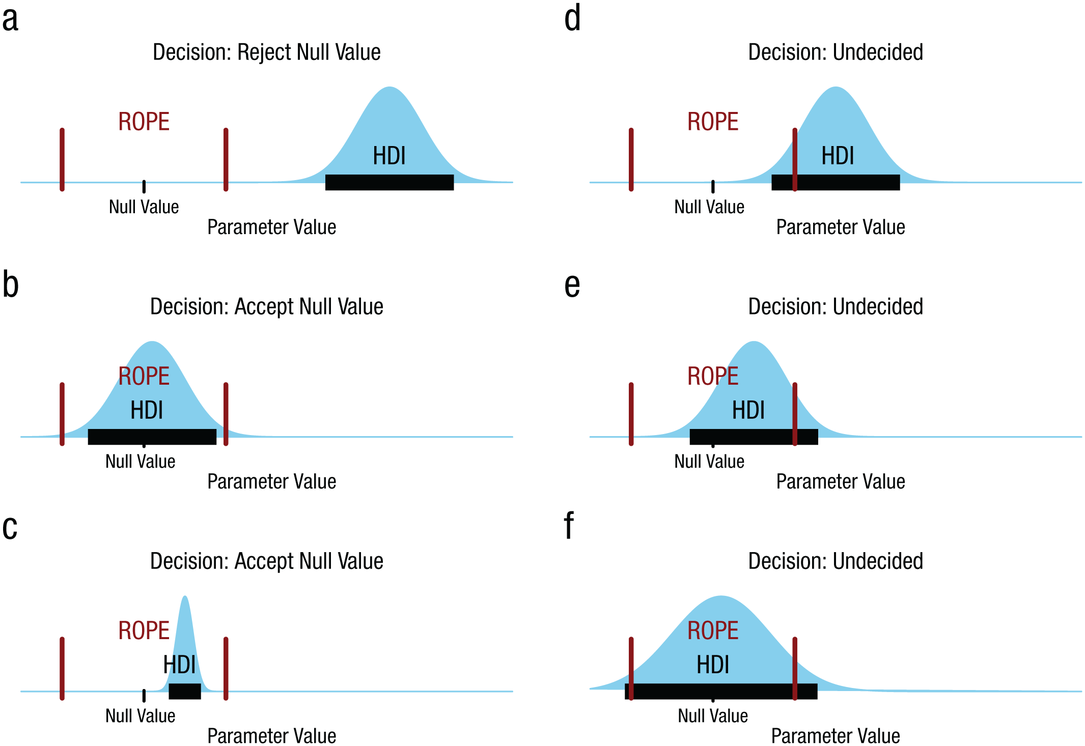
Examples of different relationships between a highest density interval (HDI) and the region of practical equivalence (ROPE), and the decisions to which they lead. In each panel, the unmarked vertical axis is probability density, the HDI is marked by the horizontal bar, and the ROPE limits are marked by the two vertical bars.

Figure 1c also shows a case in which the null value is accepted for practical purposes—here, despite the fact that the null value is not itself within the HDI. This case is important because it contrasts the meaning of the HDI (from Bayesian inference) with the meaning of the ROPE (from decision making). Accepting the null value for practical purposes does not mean that the null value is among the most credible values of the parameter distribution. Accepting the null value for practical purposes means merely that all the most credible values are practically equivalent to the null value.

The remaining panels in Figure 1 show cases in which we should remain undecided. In all three panels, some of the HDI falls outside the ROPE and some of the HDI falls inside the ROPE. Notice that we do not reject the null value in the situation depicted in Figure 1d despite the fact that the null value falls outside the HDI, because some of the HDI is practically equivalent to the null. This decision contrasts with the analogous situation in NHST: A null value is rejected if it falls outside the 95% confidence interval. We do not accept the null value in the case of Figure 1e despite the fact that the null value falls within the HDI, because some of the HDI is not practically equivalent to the null. We do not accept the null value in the case of Figure 1f despite the fact that the HDI spans the ROPE, because some of the most credible values are not equivalent to the null value.

Notice that accepting a landmark parameter value, as in the situations illustrated in Figures 1b and 1c, is not the same thing as treating the accepted value as the best estimate of the parameter value. On the contrary, the Bayesian posterior distribution indicates the estimate of the parameter value, and typically the most probable (modal) parameter value is treated as the best estimate of the parameter value. When we accept a landmark parameter value, we are merely saying that the estimate of the parameter value is close enough to the landmark value, with high enough precision, that we can treat the landmark value as good enough for practical purposes. In other words, accepting a landmark parameter value means that the best estimate of the parameter value is practically equivalent to the landmark value, not that the best estimate of the parameter value is the landmark value.

The Supplement file at the OSF (https://osf.io/jwd3t/) describes some decision-theoretic properties of the HDI+ROPE decision rule.

Numerical example

I illustrate this decision rule by applying it to a comparison of two groups for whom we have metric data (as opposed to ordinal or categorical data). Suppose the data are IQ scores from participants who have been given a placebo and participants who have been given a drug intended to make them smarter. The data within each group might have outliers, so we describe the groups with distributions that have optionally heavy tails (namely, mathematical t distributions). The model therefore has central-tendency parameters for the two groups, denoted µ₁ and µ₂; scale parameters for the two groups, denoted σ₁ and σ₂; and a normality parameter, denoted ν, that has large values for nearly normal distributions and small values for heavy-tailed distributions. The analysis begins with a broad prior distribution on the joint space of these five parameters. The broad prior is designed to have minimal influence on the form of the posterior distribution (see Kruschke, 2013, for complete details).

The data for this example were created as random numbers from normal distributions, and the sample sizes were arbitrary. The data are represented by the histograms in the upper right panels of Figure 2. The other panels of Figure 2 show aspects of the five-dimensional posterior distribution; that is, they show different perspectives of the single joint distribution. The parameter distributions were derived with Markov chain Monte Carlo methods (MCMC; see chap. 7 of Kruschke, 2015) and computed using the JAGS software (Plummer, 2003, 2017) with the runjags package in R (Denwood, 2016). HDI limits were computed from the MCMC chain using the method explained in Section 25.2.3 of Kruschke (2015) and with an effective sample size that exceeded 10,000, as recommended in Section 7.5.2 of Kruschke (2015). Complete computer code for this example is available at the OSF (https://osf.io/jwd3t/).

Fig. 2.

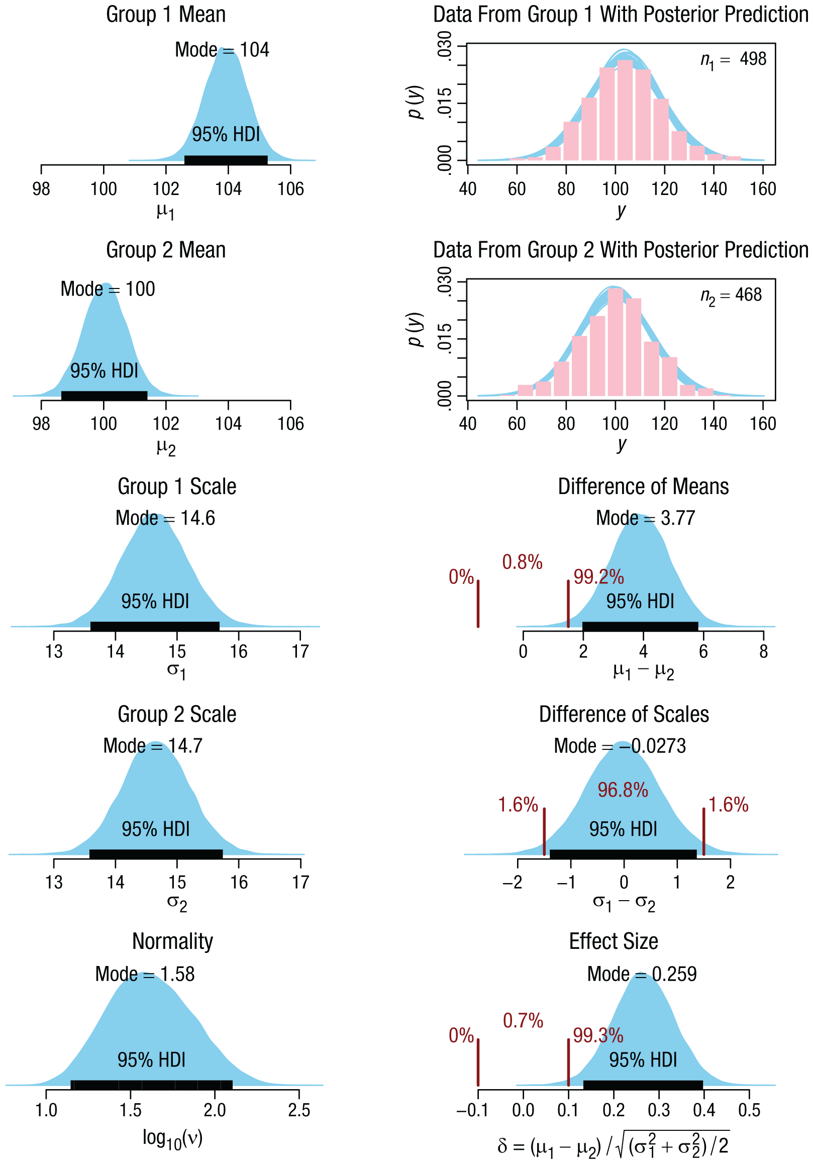
Applying the decision rule to compare two groups. The data from the groups (i.e., the IQ scores, denoted here by the generic label y) are shown as histograms in the two upper panels of the right column. Superimposed on the data histograms are t distributions predicted from the posterior distribution. The left column shows the (marginal) posterior distributions of the individual parameters in the model. The lower three panels of the right column show aspects of the posterior distribution with regions of practical equivalence (ROPEs), delimited by the vertical bars (see the main text for how the ROPE limits were selected). These panels show the percentages of the posterior distributions below the low limit of the ROPE, within the ROPE, and above the high limit of the ROPE. The 95% highest density intervals (HDIs) are indicated by the black horizontal bars. In this example, the ROPE+HDI decision rule rejects a mean difference of zero because the 95% HDI falls completely outside the ROPE, accepts a scale difference of zero because the 95% HDI falls completely inside the ROPE, and rejects an effect size of zero because the 95% HDI falls completely outside the ROPE.

In this application to two groups, it is natural to want to know the typical IQ score in each group (i.e., the magnitudes of µ₁ and µ₂), the spread of scores in each group (i.e., the magnitudes of σ₁ and σ₂), the difference in magnitude and spread between the two groups, and the uncertainty of all those estimates. We are interested in the magnitude of the difference between the means because that indicates how much IQ scores have been shifted by the smart drug, on average. We are interested in the magnitude of the difference between the spreads because that indicates how much the consistency of the scores has been affected by the smart drug. It is known, for example, that stressors can increase variability across people, as some people improve in response to a stressor whereas others decline (e.g., Lazarus & Eriksen, 1952). And of course, we are interested in the uncertainty of those estimates, so that we know how much confidence to place on their values.

The lower three panels of the right column in Figure 2 show, respectively, the posterior distribution of the difference between the means (i.e., µ₁ – µ₂), the posterior distribution of the difference between the scales (i.e., σ₁ – σ₂), and the posterior distribution of the effect size (i.e., the standardized difference between the means, calculated as $δ = (μ_{1} - μ_{2}) / \sqrt{(σ_{1}^{2} + σ_{2}^{2}) / 2}$ ; Cohen, 1988).

We can establish ROPEs on the parameters (or combinations of parameters) to make decisions. I discuss methods for setting ROPE limits later in this article, but here, for purposes of illustration, I set a ROPE on the effect size at half of Cohen’s conventional definition of a small effect, that is, at δ = ±0.1. To establish a ROPE on the difference between the means, one option is to start with the same convention as for δ and translate it to an analogous value on µ₁ – µ₂. Thus, if we assume that the standardized population value of σ is 15.0, then we can calculate the corresponding ROPE as follows: µ₁ – µ₂ = ±0.1 × 15 = ±1.5. A different option is to derive the ROPE from a real-world consideration, such as a change in mean IQ that would imply a negligible change in gross domestic product (GDP) per capita. Rindermann and Thompson (2011, p. 761) reported that a change of 1 IQ point in the population mean predicts a change of $229 in GDP per capita. If we suppose that a $687 change is practically equivalent to zero, then the ROPE would again have a width of 3 IQ points (i.e., ±1.5). Finally, for the ROPE on the difference between scales, I again used a half-width of 1.5, because σ is on the same scale as µ. This setting is merely a fallback position in the absence of specific knowledge about the utility of changes in variability, as distinct from changes in central tendency. These ROPEs are indicated in Figure 2. We decide to reject a zero difference between the means because the 95% most credible values are outside the ROPE. We also decide to reject a zero effect size. But we decide to accept a zero difference between the scales (σs) because the 95% most credible values of the difference are all practically equivalent to zero.

In summary, the posterior distribution is a multidimensional distribution on the joint parameter space, and various parameters (and combinations of parameters) can be compared simultaneously with relevant ROPEs. It is important to keep in mind that the full posterior distribution is the information delivered by Bayesian analysis, as summarized by the mode and 95% HDI of the distribution. The discrete decisions using ROPEs are secondary conclusions. Notice that to make these decisions using the HDI+ROPE rule, we must explicitly consider the magnitudes and uncertainties of the parameters; in contrast, p values and Bayes factors do not indicate the magnitudes and uncertainties of the parameters.

More About the ROPE

The ROPE in theory testing

The concept of the ROPE is useful for implementing a solution to a paradox from Meehl (1967, 1997). Theories pursued by NHST posit merely any nonnull effect and are therefore confirmed merely by rejecting the null value of the parameter, regardless of the actual magnitude of the parameter. Assuming that most variables of interest have some small but nonzero correlation with any other variable of interest, the correlation will be detected if the data set is large enough, and then the anything-but-null theory will be confirmed. Thus, anything-but-null theories incur a methodological paradox: Such theories become easier to confirm with larger sample sizes, rather than easier to disconfirm, and this is not the way scientific theories are supposed to work. By contrast, quantitatively predictive theories become easier to disconfirm with larger sample sizes because reality will almost always be somewhat discrepant from any quantitatively specific prediction. For example, the specific quantitative predictions of the Newtonian theory of gravity were disconfirmed by precise measurements of the orbit of the planet Mercury (e.g., Schiff, 1960; Will, 2014).

But how can quantitatively predictive hypotheses be confirmed? Serlin and Lapsley (1985, 1993) explained that a decision to confirm a quantitative prediction requires a ROPE (what they called a “good-enough belt”) around the predicted value. If the observed value is within the ROPE, the hypothesis is confirmed for the current practical purposes. The ROPE is a decision boundary that reflects the precision needed to distinguish current theories. If two theories make very similar predictions, then a narrow ROPE is needed to distinguish them. If two theories make rather different predictions, then a wider ROPE can be used. The ROPE also should take into account the practical meaning of the magnitude of discrepancy. In this way, when an observed value of a parameter falls within the ROPE of the predicted value, the prediction is said to be confirmed for current practical purposes.

The ROPE in equivalence testing and noninferiority testing

The concept of the ROPE is essential to frequentist equivalence testing (e.g., Lakens, 2017). In equivalence testing, the analyst specifies a ROPE around the null value and decides that the estimated parameter is statistically equivalent to the null value if the confidence interval falls entirely within the ROPE (e.g., Westlake, 1976, 1981). This decision rule follows naturally from the meanings of the confidence interval and ROPE: The confidence interval is the range of parameter values that are not rejected (e.g., Cox, 2006), and if all the unrejected values fall within the ROPE, then they are all practically equivalent to the null value.¹

The notion of the ROPE is also central to noninferiority testing (e.g., Lesaffre, 2008; Wiens, 2002), although only the low end of the ROPE is emphasized. In noninferiority testing, the analyst specifies a value below the null value that represents the largest decrease from the null value that is, nevertheless, negligible for practical purposes. The estimated value of the parameter is declared to be noninferior to the null value if that estimated value is significantly above the low end of the ROPE.

Specifying ROPE limits

How does one specify the limits of a ROPE? Because the ROPE is a decision threshold that captures practical equivalence, its limits are influenced by practical considerations, which might change through time as risks are reassessed and as theories are refined. Any decision rule must be calibrated to be useful to the audience of the analysis and to the people who are affected by the decision, and this is also true of decision rules based on p values and Bayes factors.

Equivalence testing has been used extensively in medical research, and the U.S. Food and Drug Administration (FDA) has set guidelines for the decision boundaries in equivalence testing (e.g., U.S. FDA, Center for Drug Evaluation and Research, 2001; U.S. FDA, Center for Veterinary Medicine, 2016). Recent FDA guidance for bioequivalence studies recommends ROPE limits of 0.8 and 1.25 for the ratio of means in the two groups (U.S. FDA, Center for Veterinary Medicine, 2016, p. 16). Contemporary industry standards use ROPE limits around ±20% for applications with moderate risk, but the ROPE may be narrower (i.e., ±5% to ±10%) when the risks are high, or the ROPE may be wider (i.e., ±26% to ±50%) when the risks are low (Little, 2015, Table 1).

Standards for the decision boundary of noninferiority testing have also been established by the FDA, and their recent guidance emphasizes that great care must be taken to establish the noninferiority limit because of the tremendous real-world costs and benefits of drugs and therapies (U.S. FDA, Center for Drug Evaluation and Center for Biologics Evaluation and Research, 2016). Walker and Nowacki (2011) explained that one conventional setting of the noninferiority limit is at half of “the lower limit of a confidence interval of the difference between the current therapy and the placebo obtained from a metaanalysis” (p. 194).

In many fields of science, competing theories make detailed quantitative predictions. For example, a parameter called γ should be exactly 1.0 in the theory of general relativity, but 0 in Newtonian gravity and other values near 1 in other theories (see Will, 2014, Fig. 5, p. 43, for a summary of the progression of 90 years of experiments measuring γ). A recent experiment established a value of 1 ± 0.00001 (Bertotti, Iess, & Tortora, 2003). This experiment does not merely reject Newtonian gravity (γ = 0), but confirms general relativity (γ = 1.0) even if one is using very narrow ROPEs.

In the social sciences, Cohen (1988) defined measures of effect size for different sorts of parameters and proposed conventional values for small, medium, and large effects typically observed in social-science research. In the case of the effect size of a mean, defined as δ = (µ – µ₀)/σ, Cohen suggested that 0.2 is a “small” effect, and therefore we might say that an effect is practically equivalent to zero if it is less than, say, half the size of a small effect and falls within a ROPE of ±0.1. This conventional limit was used for Figure 2.

It must be emphasized that “half the size of a small effect” is merely a fallback convention when there is no way to calibrate effects by their real-world consequences. In the case of IQ points, for instance, there might be applications for which a 0.1 effect implies nonnegligible practical consequences. A study of the GDP of 90 nations as a function of IQ and other variables found that “an increase of 1 IQ point in the intellectual class [the IQ at the 95th percentile] raises the average GDP [per capita] by $468 U.S.” (Rindermann & Thompson, 2011, p. 761). (The influence of IQ is weaker at the mean than at the 95th percentile, as mentioned earlier in the context of Fig. 2.) Thus, an increase of average IQ of the intellectual class from 130 to 131, for example, might have important consequences for GDP because that increase is multiplied across millions of people, even though an increase of 1 IQ point in any one person may be negligible for that person.

A different approach to setting the limits of a ROPE was described by Lakens (2017, p. 359), who pointed out that the maximum sample size a researcher is willing to collect data from implies, for any specific desired power, the minimal effect size that can be reliably detected. Implicitly, the sample size indicates the minimal effect size that the researcher is willing to treat as not practically equivalent to zero. This minimal effect size, in turn, implies corresponding ROPE limits for an equivalence test. I think, however, that this approach will yield ROPEs that are too wide when sample sizes are small (e.g., when research is underpowered; Maxwell, 2004) and will yield ROPEs that are too narrow when sample sizes are large (e.g., with “big data”; Adjerid & Kelley, 2018). ROPEs should be set according to the demands of competing theories and the practical implications of decisions, not by the measurement precision implied by sample size. Falling objects do not hit the ground more softly if they are measured with less precise instruments. A new drug is not more equivalent to an existing drug if it is tested for equivalence using a smaller sample size. Moreover, there are often moderate-N studies (which individually yield only moderate-precision estimates) that are worth doing even when the ROPE is relatively narrow, because future meta-analyses of multiple moderate-N studies may find a narrow meta-analytic HDI. Indeed, for random-effects models in meta-analyses, usually greater precision can be achieved by many moderate-N studies than by a few large-N studies, because hierarchical shrinkage of estimated parameter values operates more effectively (e.g., Kruschke & Liddell, 2018b; Kruschke & Vanpaemel, 2015). In meta-analyses, there is no foreknowledge of which studies will be uncovered for inclusion (from database searches of published studies and social-network searches of unpublished studies), so an analyst cannot anticipate the samples sizes or the number of studies. The ROPE must be defined from other considerations.

For parameters that have the same scale as the data, it is relatively straightforward to think about a ROPE. For example, in the case of IQ scores with a normal distribution, the mean, µ, is on the IQ scale, and its ROPE limits are in IQ points. Other models may have parameters that are less directly related to the scales of the data, and therefore ROPE limits may need to be derived more indirectly. Consider linear regression. We might want to say that a regression coefficient, β_x, is practically equivalent to zero if a change across the “main range of x” produces only a negligible change in the predicted value, $\hat{y}$ . Suppose we specify a negligible change in $\hat{y}$ as ±0.1S_y, where S_y is the standard deviation of y (a range that may be motivated by the convention that 0.1S is half of a “small” effect), and we specify the “main range of x” as M_x ± 2S_x (because if x were normally distributed, this range would cover just over 95% of the distribution). Given these specifications, a regression coefficient is practically equivalent to zero when a change of x from M_x – 2S_x to M_x + 2S_x yields a change of $\hat{y}$ only from M_y – 0.1S_y to M_y + 0.1S_y, which implies ROPE limits of β_x = ±0.05 for standardized variables. Similar considerations apply to logistic regression, as explained in the Supplement file at the OSF (https://osf.io/jwd3t/).

ROPE limits are like decision thresholds for p values and Bayes factors

In general, ROPE limits are defined by considering what counts as practically equivalent to the null value, by quantifying acceptable uncertainty as constrained by competing theories or real-world utilities. It can be challenging to specify a definitive ROPE, but one should not delude oneself into thinking that it is any more straightforward to specify a definitive decision threshold for a p value. Some people have grown comfortable with .05 as the decision threshold for a p value because it is a conventional value that statistical rituals are designed to comply with. But the convention hides the fact that there is vigorous debate about an appropriate decision threshold for p. In a recent article, Benjamin et al. (2018) argued that the threshold p value for the social sciences should be changed to .005. In physics, the contemporary conventional threshold p value corresponds to 5σ, which requires p < .00000029 for significance. Decision thresholds for p values are on no firmer ground than ROPE limits.

Bayesian null-hypothesis testing involves a decision statistic called the Bayes factor (BF). The specification of decision thresholds for BFs is as fraught as the specification of ROPEs and decision thresholds for p values. Jeffreys (1961) attached decision-strength labels to ranges of BFs as follows: 3.16 through 10.0 is “substantial,” greater than 10.0 through 31.6 is “strong,” greater than 31.6 through 100.0 is “very strong,” and greater than 100.0 is “decisive.” A subsequent influential article by Kass and Raftery (1995) suggested that BFs of 3.0 through 20.0 are “positive” evidence, BFs greater than 20.0 through 150.0 are “strong” evidence, and BFs greater than 150.0 are “very strong” evidence. In the psychological sciences, many proponents of BFs have routinely used 3 as the decision threshold (e.g., Dienes, 2016). On the other hand, Schönbrodt, Wagenmakers, Zehetleitner, and Perugini (2017) recommended a BF of 10 for mature confirmatory research but other limits for nascent research, and those authors also pointed out that different BF thresholds may apply to different types of hypothesis tests. Rouder, Morey, and Province (2013) emphasized that an extremely large BF is needed to reject null hypotheses that have a large prior probability, such as the null hypothesis that people cannot foretell the future through temporally reversed causality. Again, do not be lulled into thinking that establishing a decision threshold for Bayes factors is any easier than establishing ROPEs for HDIs.

Regardless of the decision statistic being used (p value, BF, or HDI), decision thresholds should ultimately take into account the utilities (i.e., costs and benefits) of the decisions. Unfortunately, the utilities are often unavailable. Regardless of the availability of utilities, the decision criteria should be established before the data are observed, to prevent biased decisions (e.g., Lakens et al., 2017).

Conclusion

Deciding to accept or reject a null value is dangerous, as it engenders fallacious black-and-white thinking. But when it is necessary to make such a decision, the fallacy might be fended off by focusing on explicit estimates of parameter magnitude and uncertainty. The HDI+ROPE decision method does exactly that: The analyst explicitly examines the probability distribution over parameter values and considers the relationship between the most credible parameter values and a region of practical equivalence to the null value. On the other hand, p values and BFs hide the parameter’s magnitude and uncertainty, which makes it easier to slip into specious black-and-white thinking. Setting the limits of a ROPE is no more difficult in principle than setting the decision threshold for a p value or for a BF, so researchers should be no more uncomfortable setting a ROPE than setting these other decision thresholds.

Supplemental Material

KruschkeOpenPracticesDisclosure – Supplemental material for Rejecting or Accepting Parameter Values in Bayesian Estimation

Supplemental material, KruschkeOpenPracticesDisclosure for Rejecting or Accepting Parameter Values in Bayesian Estimation by John K. Kruschke in Advances in Methods and Practices in Psychological Science

Footnotes

Acknowledgements

For comments on an early version of this article, the author gratefully acknowledges Brad Celestin and Torrin Liddell. In review and production, constructive comments were provided by Rogier Kievit, two anonymous reviewers, and Michele Nathan.

Action Editor

Daniel J. Simons served as action editor for this article.

Author Contributions

J. K. Kruschke is the sole author of this article and is responsible for its content.

Declaration of Conflicting Interests

The author(s) declared that there were no conflicts of interest with respect to the authorship or the publication of this article.

Open Practices

The R code for the example in Figure 2 has been made publicly available via the Open Science Framework and can be accessed at https://osf.io/jwd3t/. The complete Open Practices Disclosure for this article can be found at http://journals.sagepub.com/doi/suppl/10.1177/2515245918771304. This article has received the badge for Open Materials. More information about the Open Practices badges can be found at .

Notes

References

Adjerid

Kelley

(2018). Big data in psychology: A framework for research advancement. American Psychologist. Advance online publication. doi:10.1037/amp0000190

Bayes

Price

(1763). An essay towards solving a problem in the doctrine of chances. By the late Rev. Mr. Bayes, F. R. S. Communicated by Mr. Price, in a letter to John Canton, A. M. F. R. S. Philosophical Transactions, 53, 370–418. doi:10.1098/rstl.1763.0053

Benjamin

D. J.

Berger

J. O.

Johannesson

Nosek

B. A.

Wagenmakers

E.-J.

Berk

. . . Johnson

V. E

(2018). Redefine statistical significance. Nature Human Behavior, 2, 6–10. doi:10.1038/s41562-017-0189-z

Bertotti

Iess

Tortora

(2003). A test of general relativity using radio links with the Cassini spacecraft. Nature, 425, 374–376. doi:10.1038/nature01997

Carlin

B. P.

Louis

T. A.

(2009). Bayesian methods for data analysis (3rd ed.). Boca Raton, FL: CRC Press.

Cohen

(1988). Statistical power analysis for the behavioral sciences (2nd ed.). Hillsdale, NJ: Erlbaum.

Cox

D. R.

(2006). Principles of statistical inference. Cambridge, England: Cambridge University Press.

Cumming

(2014). The new statistics: Why and how. Psychological Science, 25, 7–29.

Denwood

M. J.

(2016). runjags: An R package providing interface utilities, model templates, parallel computing methods and additional distributions for MCMC models in JAGS. Journal of Statistical Software, 71(9), 1–25. doi:10.18637/jss.v071.i09

10.

Dienes

(2016). How Bayes factors change scientific practice. Journal of Mathematical Psychology, 72, 78–89. doi:10.1016/j.jmp.2015.10.003

11.

Freedman

L. S.

Lowe

Macaskill

(1984). Stopping rules for clinical trials incorporating clinical opinion. Biometrics, 40, 575–586.

12.

Hobbs

B. P.

Carlin

B. P.

(2008). Practical Bayesian design and analysis for drug and device clinical trials. Journal of Biopharmaceutical Statistics, 18, 54–80.

13.

Jeffreys

(1961). Theory of probability (3rd ed.). Oxford, England: Oxford University Press.

14.

Kappel

Fisher-Fleming

Hogue

E. J.

(1995). Ideal pear sensory attributes and fruit characteristics. HortScience, 30, 988–993.

15.

Kappel

Fisher-Fleming

Hogue

E. J.

(1996). Fruit characteristics and sensory attributes of an ideal sweet cherry. HortScience, 31, 443–446.

16.

Kass

R. E.

Raftery

A. E.

(1995). Bayes factors. Journal of the American Statistical Association, 90, 773–795.

17.

Kruschke

J. K.

(2010). Bayesian data analysis. Wiley Interdisciplinary Reviews: Cognitive Science, 1, 658–676. doi:10.1002/wcs.72

18.

Kruschke

J. K.

(2011a). Bayesian assessment of null values via parameter estimation and model comparison. Perspectives on Psychological Science, 6, 299–312.

19.

Kruschke

J. K.

(2011b). Doing Bayesian data analysis: A tutorial with R and BUGS (1st ed.). Burlington, MA: Academic Press.

20.

Kruschke

J. K.

(2013). Bayesian estimation supersedes the t test. Journal of Experimental Psychology: General, 142, 573–603. doi:10.1037/a0029146

21.

Kruschke

J. K.

(2015). Doing Bayesian data analysis: A tu-torial with R, JAGS, and Stan (2nd ed.). Burlington, MA: Academic Press.

22.

Kruschke

J. K.

Aguinis

Joo

(2012). The time has come: Bayesian methods for data analysis in the organizational sciences. Organizational Research Methods, 15, 722–752. doi:10.1177/1094428112457829

23.

Kruschke

J. K.

Liddell

T. M.

(2018a). Bayesian data analysis for newcomers. Psychonomic Bulletin & Review, 25, 155–177. doi:10.3758/s13423-017-1272-1

24.

Kruschke

J. K.

Liddell

T. M.

(2018b). The Bayesian new statistics: Hypothesis testing, estimation, meta-analysis, and power analysis from a Bayesian perspective. Psychonomic Bulletin & Review, 25, 178–206. doi:10.3758/s13423-016-1221-4

25.

Kruschke

J. K.

Vanpaemel

(2015). Bayesian estimation in hierarchical models. In Busemeyer

J. R.

Wang

Townsend

J. T.

Eidels

(Eds.), The Oxford handbook of computational and mathematical psychology (pp. 279–299). Oxford, England: Oxford University Press.

26.

Lakens

(2014). Performing high-powered studies efficiently with sequential analyses. European Journal of Social Psychology, 44, 701–710.

27.

Lakens

(2017). Equivalence tests: A practical primer for t tests, correlations, and meta-analyses. Social Psychological & Personality Science, 8, 355–362.

28.

Lakens

Adolfi

Albers

Anvari

Apps

Argamon

. . . Zwaan

(2017). Justify your alpha. Retrieved from https://psyarxiv.com/9s3y6

29.

Lazarus

R. S.

Eriksen

C. W.

(1952). Effects of failure stress upon skilled performance. Journal of Experimental Psychology, 43, 100–105. doi:10.1037/h0056614

30.

Lesaffre

(2008). Superiority, equivalence, and non-inferiority trials. Bulletin of the NYU Hospital for Joint Diseases, 66, 150–154.

31.

Little

T. A.

(2015). Equivalence testing for comparability. BioPharm International, 28(2), 45–48.

32.

Maxwell

S. E.

(2004). The persistence of underpowered studies in psychological research: Causes, consequences, and remedies. Psychological Methods, 9, 147–163.

33.

Meehl

P. E.

(1967). Theory-testing in psychology and physics: A methodological paradox. Philosophy of Science, 34, 103–115.

34.

Meehl

P. E.

(1997). The problem is epistemology, not statistics: Replace significance tests by confidence intervals and quantify accuracy of risky numerical predictions. In Harlow

L. L.

Mulaik

S. A.

Steiger

J. H.

(Eds.), What if there were no significance tests? (pp. 395–425). Mahwah, NJ: Erlbaum.

35.

Plummer

(2003). JAGS: A program for analysis of Bayesian graphical models using Gibbs sampling. In Hornik

Leisch

Zeileis

(Eds.), Proceedings of the 3rd International Workshop on Distributed Statistical Computing (DSC 2003). Retrieved from https://www.r-project.org/conferences/DSC-2003/Proceedings/Plummer.pdf

36.

Plummer

(2017). JAGS Version 4.3.0 user manual. Retrieved from https://sourceforge.net/projects/mcmc-jags/files/Manuals/4.x/jagsusermanual.pdf/download

37.

Rindermann

Thompson

(2011). Cognitive capitalism: The effect of cognitive ability on wealth, as mediated through scientific achievement and economic freedom. Psychological Science, 22, 754–763.

38.

Rouder

J. N.

Morey

R. D.

Province

J. M.

(2013). A Bayes factor meta-analysis of recent extrasensory perception experiments: Comment on Storm, Tressoldi, and Di Risio (2010). Psychological Bulletin, 139, 241–247.

39.

Schiff

L. I.

(1960). On experimental tests of the general theory of relativity. American Journal of Physics, 28, 340–343. doi:10.1119/1.1935800

40.

Schönbrodt

F. D.

Wagenmakers

E.-J.

Zehetleitner

Perugini

(2017). Sequential hypothesis testing with Bayes factors: Efficiently testing mean differences. Psychological Methods, 22, 322–339.

41.

Schuirmann

D. J.

(1987). A comparison of the two one-sided tests procedure and the power approach for assessing the equivalence of average bioavailability. Journal of Pharmacokinetics and Biopharmaceutics, 15, 657–680.

42.

Serlin

R. C.

Lapsley

D. K.

(1985). Rationality in psychological research: The good-enough principle. American Psychologist, 40, 73–83.

43.

Serlin

R. C.

Lapsley

D. K.

(1993). Rational appraisal of psychological research and the good-enough principle. In Keren

Lewis

(Eds.), A handbook for data analysis in the behavioral sciences: Methodological issues (pp. 199–228). Mahwah, NJ: Erlbaum.

44.

Spiegelhalter

D. J.

Freedman

L. S.

Parmar

M. K. B.

(1994). Bayesian approaches to randomized trials. Journal of the Royal Statistical Society: Series A, 157, 357–416.

45.

U.S. Food and Drug Administration, Center for Drug Evaluation and Research. (2001). Guidance for industry: Statistical approaches to establishing bioequiva-lence. Retrieved from https://www.fda.gov/downloads/drugs/guidances/ucm070244.pdf

46.

U.S. Food and Drug Administration, Center for Drug Evaluation and Research and Center for Biologics Evaluation and Research. (2016). Non-inferiority clinical trials to establish effectiveness: Guidance for industry. Retrieved from https://www.fda.gov/downloads/drugs/guidancecomplianceregulatoryinformation/guidances/ucm202140.pdf

47.

U.S. Food and Drug Administration, Center for Veterinary Medicine. (2016). Guidance for industry: Bioequivalence: Blood level bioequivalence study VICH GL52. Re-trieved from https://www.fda.gov/downloads/AnimalVeterinary/GuidanceComplianceEnforcement/GuidanceforIndustry/UCM415697.pdf

48.

Walker

Nowacki

A. S.

(2011). Understanding equivalence and noninferiority testing. Journal of General Internal Medicine, 26, 192–196.

49.

Wasserstein

R. L.

Lazar

N. A.

(2016). The ASA’s statement on p-values: Context, process, and purpose. The American Statistician, 70, 129–133. doi:10.1080/00031305.2016.1154108

50.

Westlake

W. J.

(1976). Symmetrical confidence intervals for bioequivalence trials. Biometrics, 32, 741–744.

51.

Westlake

W. J.

(1981). Response to bioequivalence testing—a need to rethink. Biometrics, 37, 591–593.

52.

Wiens

B. L.

(2002). Choosing an equivalence limit for noninferiority or equivalence studies. Controlled Clinical Trials, 23, 2–14.

53.

Will

C. M.

(2014). The confrontation between general relativity and experiment. Living Reviews in Relativity, 17, Article 4. doi:10.12942/lrr-2014-4

Supplementary Material

Please find the following supplemental material available below.

For Open Access articles published under a Creative Commons License, all supplemental material carries the same license as the article it is associated with.

For non-Open Access articles published, all supplemental material carries a non-exclusive license, and permission requests for re-use of supplemental material or any part of supplemental material shall be sent directly to the copyright owner as specified in the copyright notice associated with the article.

0.00 MB

0.64 MB