Sage Journals: Discover world-class research

Abstract

Longitudinal studies with time-varying treatments or exposures make it hard to figure out “what effect” is being estimated. Drawing on causal inference, we clarify this by distinguishing between total, direct, and—centrally—joint effects, defined within the potential-outcomes framework and illustrated with directed acyclic graphs. Joint effects extend average treatment effects to repeated interventions, providing a practical measure of combined intervention effects over time. Using a worked example on smartphone use and sleep quality, we demonstrate how different estimands answer different questions, why single total effects can sometimes mislead in longitudinal settings, and how joint effects capture strategy-level consequences across time. A key practical takeaway is that joint effects can be estimated in both experimental and observational studies. In the latter, it typically suffices to adjust only for variables that govern treatment decisions at each time point rather than modeling the entire causal system. Building on this, we propose covariate-driven treatment assignment (information-restriction designs in which decisions depend only on observed covariates) as a practical route to causal inference in nonexperimental psychology, and we connect these designs to estimation via g-methods from epidemiology. We provide open materials, including R code, to support adoption.

Keywords

causal inference longitudinal research time-varying treatments causal estimands joint effects g-methods psychology estimand g-formula media potential outcomes sleep open materials

Psychologists are increasingly interested in longitudinal study designs, driven by the desire to gain a deeper understanding of how psychological processes unfold over time (Baumert et al., 2017; Ebner Priemer et al., 2009). This growing interest has been fueled, in part, by the advent of novel data-collection techniques, including experience-sampling and mobile-sensing methods (Harari et al., 2016; Schoedel & Mehl, 2024; Wrzus & Neubauer, 2023). Alongside this development, psychological methodology has increasingly incorporated causal-estimation approaches from other disciplines, such as epidemiology and econometrics (Chatton & Rohrer, 2024; Grosz et al., 2024; Rohrer, 2018). In this context, methodological researchers have called for clearer communication of the causal estimand (i.e., the mathematical quantity that answers a causal research question; Auspurg & Brüderl, 2021; Lundberg et al., 2021) and greater precision in specifying the assumptions required for causal inference (Bailey et al., 2024). However, this body of research has focused predominantly on nonlongitudinal outcomes. As a result, there remains a gap in the integration of causal-inference methods for longitudinal data in psychological research (Bailey et al., 2024; Rohrer & Murayama, 2023).

The distinguishing feature of longitudinal designs in the context of causal inference is that treatment-outcome relationships are evaluated repeatedly over time, resulting in many possible estimands that researchers might be interested in. Rohrer and Murayama (2023) called for greater clarity in longitudinal settings because vague verbal theories lead to multiple possible estimands (for an example from cross-sectional research, see Auspurg & Brüderl, 2021). Articulating temporally precise theories and connecting them to statistical methods is essential in longitudinal designs (Hopwood et al., 2022). But this is achievable only if psychological researchers (a) are aware of the different estimands and (b) clearly specify their target estimand.

For this purpose, in the present article, we provide a conceptual introduction to the different causal estimands that can arise in longitudinal settings. In particular, we describe a class of estimands known as “joint effects.” These joint effects quantify how well an intervention or a treatment works when it is administered multiple times over a period of time. Their effectiveness is evaluated based on later outcomes, allowing for the comparison of temporal dependencies. Conceptually, joint effects allow researchers to address questions such as the following: Should a patient attend all therapy sessions (i.e., receive every treatment)? Is it sufficient to begin therapy later (i.e., receive only later treatments)? Or is it preferable to forgo therapy entirely (i.e., receive no treatment)?

Joint effects were first conceptualized in epidemiology, in which they remain the predominant estimand in longitudinal designs (Hernán & Robins, 2020; Robins, 1986). They have recently gained traction in psychology through a series of rather technical tutorial articles: Researchers have demonstrated how joint effects can be formulated in linear structural equation models (SEMs; Mulder et al., 2024, 2025)¹ and how SEM software can be used to implement different estimation strategies for joint effects (Loh et al., 2024; Loh & Ren, 2023). However, this literature devotes little attention to the underlying concept of the estimand itself or to the scenarios in which it can be meaningfully estimated. Instead, the focus is on what to do once joint effects have been selected as the target estimand and their identification is ensured.

Although psychology has a long tradition of modeling longitudinal data using SEMs (Usami et al., 2019), joint effects have rarely been treated as compelling estimands. We believe that more researchers would be interested in joint effects if they understood their meaning and usefulness more clearly. In this article, we bridge that gap by offering a concise, nontechnical introduction to what joint effects are and why they matter for psychologists. To that end, we develop a hypothetical longitudinal study to show how to identify and interpret joint effects, and we provide R code for simulation and estimation in the online supplement (https://osf.io/eczky/). We then discuss the practical value of joint effects, emphasizing that they can often be estimated under weaker confounding assumptions than methods commonly used in observational psychological research. Joint effects typically require adjustment only for variables that govern treatment decisions, and researchers do not need to know all variables in the causal system. We introduce a class of research designs that leverage this property. First, however, we present a conceptual overview of causal inference for longitudinal data using potential outcomes and causal graphs.

Introduction to Causal-Inference Tools

Quantitative causal reasoning usually follows a road map (see Dang et al., 2023; Lawes et al., 2025) that can be grouped into three broader stages. The first stage involves defining a quantifiable causal estimand: the quantity one wants to estimate (Lundberg et al., 2021). Once this target estimand is specified, the next stage is to articulate the assumptions necessary to identify the estimand and connect it to the available data. Finally, the third stage is to develop a statistical model that estimates the causal estimand.

In this article, we primarily focus on clarifying the first and second stages in the context of psychological-research scenarios. Our focus is not on the third stage, although we present one approach for estimating longitudinal effects in the online supplement.

Stage 1: defining the causal estimand of interest

Specifying the estimand is the foundational step in causal inference (Lundberg et al., 2021). It is essential to first state which causal effect one intends to investigate before describing the techniques used for its estimation (Rubin, 2005). In causal inference, these target quantities that answer the research question of interest are called “causal estimands.” For example, if a researcher is interested in how effective a drug is in relieving headaches, a corresponding causal estimand is the variable that addresses the following question: What is the quantitative difference in headache severity if a person takes the drug versus if the person does not?

Causal estimands become more difficult to conceptualize in longitudinal settings. In these contexts, numerous causal estimands can arise simply because there are many time points that can be compared. For instance, researchers might be interested in the effect of taking the drug only at a specific time point $t$ . They might also examine the effect of sustained drug treatment at all time points compared with treatment only during the early or later phases or no treatment at all.

A causal estimand represents the effect of actions or interventions and is therefore not merely a description of statistical models or coefficients. Thus, causal estimands require a distinct language. One predominant framework for formulating causal estimands is the potential-outcomes framework (POF; Neyman, 1923/1990; Rubin, 1974).

The potential-outcomes framework is a general framework for causal inference that is widely used in both epidemiology and economics (Hernán & Robins, 2020; Imbens, 2020). Psychologists may find this perspective on causality intuitive because it is based directly on an experimental point of view (Eronen, 2020; Rohrer & Lucas, 2020). The basic idea is that before a treatment ( $A$ ) is administered, a participant has two potential outcomes: $Y^{a = 1}$ in the treatment condition ( $a = 1$ ; read: the potential outcome of $Y$ for an individual under treatment $a = 1$ ) and $Y^{a = 0}$ under no treatment ( $a = 0$ ). The individual causal effect of a person is the difference between these two outcomes, $Y^{a = 1} - Y^{a = 0}$ .

As an example, consider the question of whether smartphone usage affects sleep quality. Let $Y^{a = 0}$ represent the sleep quality of a person on a day without smartphone usage and $Y^{a = 1}$ represent the sleep quality on the same day if the person used a smartphone at least once. After a poor night of sleep, the person may wonder, “What would my sleep quality have been like if I had not used my smartphone yesterday?” This question implies that all other conditions on that day remained identical except for smartphone usage. We denote this difference as $Y^{a = 1} - Y^{a = 0}$ .

Because only one potential outcome can be observed for each person, we cannot know individual causal effects (Holland, 1986). But we can still reason about the average treatment effect (ATE): the mean difference between sleep quality if everyone used their smartphone and if no one did, defined as $E [Y^{a = 1} - Y^{a = 0}]$ . The expectation aggregates the individual treatment effects into a single number—the causal estimand (Lundberg et al., 2021). This “total effect” of a treatment is a particularly important causal estimand because it is the quantity that can be estimated in an ideal randomized controlled trial (RCT) without bias (Ohlsson & Kendler, 2020).

In longitudinal study designs with time-varying treatments, a treatment $a_{t}$ is not administered only once but repeatedly over time ( $t = 1, \dots, T$ ). For example, researchers can divide a day into (e.g., hourly) bins and assess the effect of smartphone usage $a_{t}$ on sleep quality $Y$ for every time point $t$ . To keep the example simple, we primarily focus on settings in which the outcome $Y$ (in our case, sleep quality) is evaluated only once at the end of the study.

From a temporal perspective, potential outcomes depend on when the intervention occurs and when the outcome is assessed. We can consider distinct interventions at each time point. $Y^{a_{t}}$ denotes the potential outcome if smartphone usage was intervened on only at time point $t$ . If we view these interventions $a_{t}$ separately, we obtain a distinct end-of-study potential outcome for intervening at each time point: $Y^{a_{1}}, Y^{a_{2}}, \dots, Y^{a_{T}}$ . Alternatively, we can combine all interventions and conceptualize potential outcomes under a specific sequence of treatment interventions (Robins, 1986, 1997). In this case, we propose a counterfactual scenario in which the intervention occurs at each time point $t$ according to a specific sequence. For example, one possible sequence could involve using a smartphone during the morning hours but not during the evening hours.

This sequence of treatments is called a treatment “regime” or “strategy,” denoted by $\bar{a}$ (read: “a bar”). If we consider the treatment “smartphone usage” as binary, the phone can either be used or not at each time point $t$ . This results in $2^{T}$ possible strategies—one for each combination at time points $t = 1, \dots, T$ . Accordingly, there are $2^{T}$ potential outcomes, $Y^{\bar{a}}$ , one for each strategy.

For simplicity, in this article, we focus on static treatment strategies in which treatment assignment is fixed in advance for all $t$ s and is followed regardless of potential changes in other covariates. One conceptually important static strategy in many practical settings (e.g., psychotherapeutic settings) is to “always treat,” in which case, the treatment is administered at every time point. The sequence of values that represents this strategy is $\bar{a} = (1, 1, 1, \dots, 1) = \bar{1}$ . The individual potential outcome $Y^{\bar{a} = \bar{1}}$ of this longitudinal treatment strategy $\bar{a} = \bar{1}$ for some participant corresponds to a what-if statement: “What outcome would we observe if the participant followed the treatment strategy $\bar{a} = \bar{1}$ (e.g., used a smartphone at every time point $t$ )?”

The causal effect of a treatment strategy on the outcome—the difference in the outcome under two longitudinal treatment strategies—is called the “joint effect” of a treatment strategy (Elwert, 2013). The term “joint” highlights that multiple treatments are administered, and their combined effect on the outcome $Y$ is evaluated. The term “effect” signifies that this is a causal quantity, representing a contrast between two potential outcomes. At the population level, the most prominent extension of the ATE in our longitudinal setting is the comparison between the two strategies “always treat” and “never treat”: $E [Y^{\bar{a} = \bar{1}} - Y^{\bar{a} = \bar{0}}]$ , with $\bar{0} = (0, 0, 0, \dots, 0)$ .

Therefore, one way to think about joint effects is to view them as the result of an RCT in which two complete strategies are compared. Alternatively, joint effects can be understood as the combination of individual treatment effects at each time point. This perspective is crucial for interpreting joint effects and also makes it possible to learn them from observational data rather than only from experiments (Daniel et al., 2013). We further elaborate on these points and provide guidance on their identification in a later section of this article.

Stage 2: identification of the estimand

After defining the causal estimand of interest, the second stage of causal inference is identification. Identification asks which causal assumptions are necessary to link the hypothetical estimand to the observed data (consistency, exchangeability, and positivity; see Hernán & Robins, 2020). In this article, we focus only on the assumption of exchangeability (Hernán & Robins, 2020), also called “unconfoundedness” (Imbens & Rubin, 2015), which concerns the structure of confounding variables. We need to assume that differences in sleep quality are due to only different smartphone usage and not a common cause of the two. For example, younger people use their smartphone more often yet have different sleep patterns than older adults. In experimental settings, researchers assume that confounding variables are controlled through randomization. In nonexperimental settings, researchers assume that confounding can be mitigated by measuring relevant variables and adjusting for them in a statistical model.

We stress this assumption about unconfoundedness in this article because of the key advantage that joint effects do not require every confounder to be measured but, rather, only a specific subset of them (Richardson & Robins, 2013). Generally, the step of identification becomes challenging in longitudinal studies because there are multiple variables and interactions between them. Using one’s phone at time point $t$ may influence the effect of future usage at $t + 1$ , the willingness to use the phone again, and other time-varying variables that affect sleep quality, such as rumination. This creates time-dependent confounding, which must be addressed at every time point $t$ . A useful way to visualize this structure is via causal directed acyclic graphs (DAGs; Hernán & Robins, 2020).

DAGs are a valuable tool in causal inference because they visually represent a researcher’s beliefs about the causal process. Their benefits are well established (Pearl, 2009), and intuitive introductions for psychologists are available (Rohrer, 2018).² In a DAG, relevant variables (denoted here as $L$ ) may serve as confounders, colliders, or mediators between the causal effect of the treatment $A$ on the outcome $Y$ . A confounder (e.g., age or rumination) is a cause of both treatment and outcome ( $A \leftarrow L \to Y$ ). A collider (e.g., mood the next day) is caused by both treatment and outcome ( $A \to L \leftarrow Y$ ). A mediator (e.g., blue-light exposure) lies on the causal pathway between treatment and outcome, that is, is caused by the treatment and is a cause of the outcome ( $A \to L \to Y$ ).

DAGs help researchers to determine which variables need to be controlled for to identify a causal effect of interest (Cinelli et al., 2024; Poppe et al., 2025). Confounders must be adjusted for, and adjusting for colliders introduces bias. Whether it is appropriate to adjust for mediators depends on the estimand. Ultimately, the identification of causal effects relies on independence assumptions between variables. 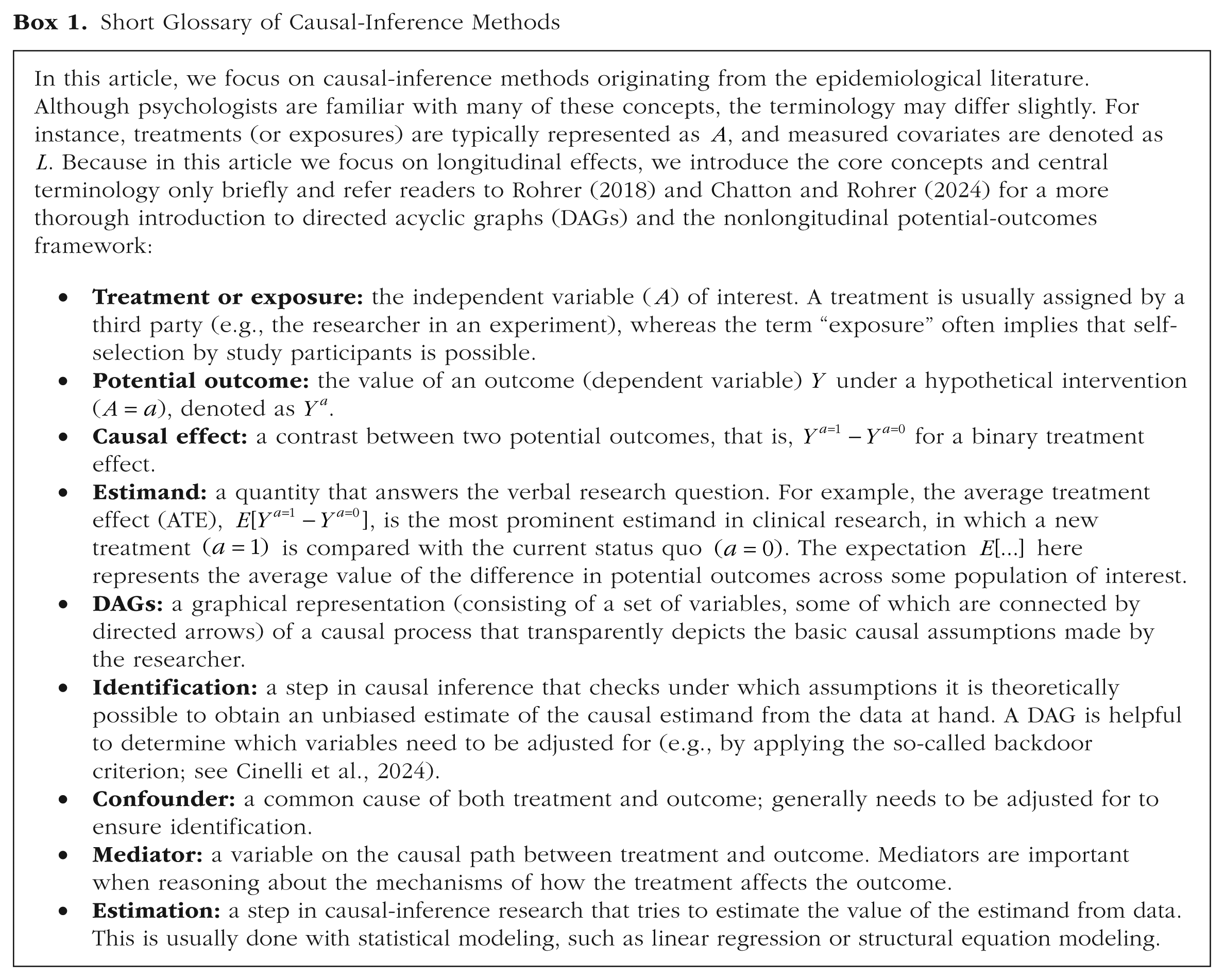These independence assumptions come in two forms, which can be depicted in a DAG (Pearl, 2009): First, assume that conditional on observed confounders, there is no unmeasured common cause $U$ between two variables (i.e., no U such that $A \leftarrow U \to Y$ ). This is the graphical way to state the assumption of unconfoundedness. Another independence assumption is conveyed if no directed arrow is drawn between two variables. Then, the direct causal effect is exactly zero, conditional on observed mediators. Note that omitting a path in a DAG is always a stronger assumption than suggesting that the path may exist (Poppe et al., 2025). Assuming a nonzero path is weaker because this makes no claims about the strength or the functional form of the effect (Bollen & Pearl, 2013).

DAGs are particularly useful in longitudinal designs involving many time-varying variables because some of these variables may act as both confounders and colliders at the same time (Hernán & Robins, 2020). Moreover, prior treatments typically serve as confounders for subsequent treatment effects because they influence both the likelihood of receiving later treatments and the outcome. In the next section, we illustrate this concept alongside the other concepts discussed here using a running example. For a brief review of the terminology, see Box 1.

Box 1.

Short Glossary of Causal-Inference Methods

In this article, we focus on causal-inference methods originating from the epidemiological literature. Although psychologists are familiar with many of these concepts, the terminology may differ slightly. For instance, treatments (or exposures) are typically represented as

A

, and measured covariates are denoted as

L

. Because in this article we focus on longitudinal effects, we introduce the core concepts and central terminology only briefly and refer readers to Rohrer (2018) and Chatton and Rohrer (2024) for a more thorough introduction to directed acyclic graphs (DAGs) and the nonlongitudinal potential-outcomes framework:
• Treatment or exposure: the independent variable (

A

) of interest. A treatment is usually assigned by a third party (e.g., the researcher in an experiment), whereas the term “exposure” often implies that self-selection by study participants is possible.
• Potential outcome: the value of an outcome (dependent variable)

Y

under a hypothetical intervention (

A = a

), denoted as

Y^{a}

.
• Causal effect: a contrast between two potential outcomes, that is,

Y^{a = 1} - Y^{a = 0}

for a binary treatment effect.
• Estimand: a quantity that answers the verbal research question. For example, the average treatment effect (ATE),

E [Y^{a = 1} - Y^{a = 0}]

, is the most prominent estimand in clinical research, in which a new treatment

(a = 1)

is compared with the current status quo

(a = 0)

. The expectation

E [\dots]

here represents the average value of the difference in potential outcomes across some population of interest.
• DAGs: a graphical representation (consisting of a set of variables, some of which are connected by directed arrows) of a causal process that transparently depicts the basic causal assumptions made by the researcher.
• Identification: a step in causal inference that checks under which assumptions it is theoretically possible to obtain an unbiased estimate of the causal estimand from the data at hand. A DAG is helpful to determine which variables need to be adjusted for (e.g., by applying the so-called backdoor criterion; see Cinelli et al., 2024).
• Confounder: a common cause of both treatment and outcome; generally needs to be adjusted for to ensure identification.
• Mediator: a variable on the causal path between treatment and outcome. Mediators are important when reasoning about the mechanisms of how the treatment affects the outcome.
• Estimation: a step in causal-inference research that tries to estimate the value of the estimand from data. This is usually done with statistical modeling, such as linear regression or structural equation modeling.

Causal Inference in Longitudinal Studies: An Illustrative Example

As already mentioned in the previous section, some challenges arise when conducting causal inference in longitudinal study designs. To explain these challenges in more detail and to illustrate the definition (Stage 1) and identification (Stage 2) of causal estimands in longitudinal settings, we use a running example based on a hypothetical RCT. This example is motivated by the question of whether smartphone usage affects sleep quality and in particular, whether usage that occurs well before bedtime already influences sleep.

In this RCT, participants are randomly assigned to use a specific social media app from 8 p.m. to 10 p.m. ( $t = 1$ ) or not. There is no intervention afterward, meaning that from 10 p.m. to midnight ( $t = 2$ ), participants can decide for themselves whether to use this app, and this usage is passively recorded. We set $a_{t} = 1$ if the social media app was used during the time frame indexed by $t$ , and $a_{t} = 0$ means that the app was not used at all during $t$ . At 10 p.m., participants’ rumination ( $L$ ) is also measured because it is hypothesized to be another mediator between social media usage and sleep quality. The final outcome of the study, sleep quality ( $Y$ ), is measured the next morning. Figure 1 presents a DAG corresponding to this RCT. Because early social media usage was manipulated in an experiment, there are no arrows pointing into $A_{1}$ . In contrast, $A_{2}$ can be influenced by both $A_{1}$ and $L$ . The variable $U$ represents the set of all unmeasured confounders. Note that in our example, we make the strong assumption that $U$ is not a direct cause of $A_{2}$ , and we discuss this potentially implausible assumption in the later section on identification.

Fig. 1.

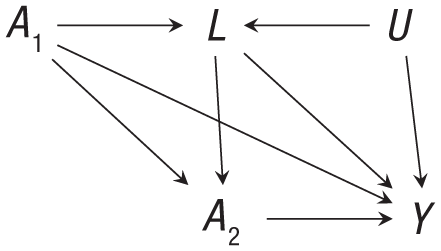
Directed acyclic graph that represents the running example. $U$ represents the set of all unmeasured confounders, and $L$ and $A_{2}$ are measured mediators of the causal effect of $A_{1}$ on the end of study outcome $Y$ .

In our online supplementary material, we use this example to demonstrate how to specify a data-generating process that aligns with the DAG presented in Figure 1 and how to determine the true expected potential outcomes and corresponding causal effects by simulating data from this process. The supplementary materials, including the R code, are available in our OSF repository (https://osf.io/eczky/). For a more convenient reading experience, we also present our supplementary materials as a website (https://florianpargent.github.io/joint_effects_ampps/).

Stage 1: defining the causal estimand of interest in longitudinal study designs

The overarching research question of whether using a social media app affects sleep quality leads to multiple estimands of interest in a longitudinal setting. In particular, one can distinguish between different estimands that can be of interest, depending on the respective research questions: total effects, joint effects, or direct effects (Daniel et al., 2013).

Total effects

It is well known that RCTs offer a way to estimate certain causal effects by leveraging randomization: Because $A_{1}$ is randomly assigned, it cannot be affected by other variables (no arrows point to $A_{1}$ ). The observed mean difference in sleep quality between study groups is an unbiased estimate for the causal effect of social media usage at $t = 1$ , that is, E[ $Y^{a_{1} = 0}] = E [Y^{a_{1} = 1}] - E [Y^{a_{1} = 0}]$ . Because the intervention occurred only at the beginning, this contrast captures all causal paths—both direct and indirect—from $A_{1}$ to $Y$ and is therefore referred to as the “total effect” (Daniel et al., 2013). More generally, the total effect of $A_{t}$ represents the impact of a single-point intervention at time $t$ on a later outcome $Y$ , $E [Y^{a_{t} = 1} - Y^{a_{t} = 0}]$ .

In longitudinal settings, the strength and direction of total effects can strongly depend on the time point of the intervention and the time point when the outcome is measured. $A_{2}$ corresponds to social media usage between 10 p.m. and midnight that was not randomly assigned. In our example, we assume that social media usage right before bedtime ( $A_{2}$ ) negatively affects sleep quality directly and that earlier usage ( $A_{1}$ ) has only a small negative direct effect. However, early usage reduces the likelihood of later use, thereby indirectly improving sleep quality. This dynamic results in a net positive total effect of early social media usage.

In our hypothetical study, the researchers uncover this unexpected result (see Supplement 2 online, https://florianpargent.github.io/joint_effects_ampps/supplement_2.html): The total effect of social media usage at $A_{1}$ appears to be small but positive, suggesting that using the phone earlier in the evening improves sleep quality. The researchers speculate that this is somehow connected to later social media usage $A_{2}$ and rumination $L$ . They now want to assess whether a later intervention might be more beneficial or whether people should, rather, not use social media for the whole evening if they want to improve their sleep. In this case, simply randomizing at a single time point and comparing outcomes is not sufficient. The researchers must consider the effects of joint interventions (VanderWeele, 2021).

Joint effects

The first joint effect that researchers may wish to investigate is the effectiveness of the strategies “always treat” versus “never treat”: $E [Y^{\bar{a} = \bar{1}} - Y^{\bar{a} = \bar{0}}]$ . This corresponds to a contrast between the intervention groups, assuming that the “social media usage” group continues to use their phone at both time points $(a_{1} = 1, a_{2} = 1)$ and the “no social media usage” group continues to abstain $(a_{1} = 0, a_{2} = 0)$ . This joint effect compares the two most extreme treatment strategies. However, other possible joint effects may also be of interest: With two time points, there are four possible treatment strategies, which all can be contrasted: $(a_{1} = 0, a_{2} = 0)$ , $(a_{1} = 1, a_{2} = 0)$ , $(a_{1} = 0, a_{2} = 1)$ , and $(a_{1} = 1, a_{2} = 1)$ .

For example, the researchers may want to assess whether early social media usage at $t = 1$ affects sleep quality independently of later usage at $t = 2$ . To evaluate this using potential outcomes, one can fix social media usage at $t = 2$ to zero ( $a_{2} = 0$ ) and compare different levels of early social media usage. The corresponding potential-outcome contrast is then $E [Y^{a_{1} = 1, a_{2} = 0} - Y^{a_{1} = 0, a_{2} = 0}]$ , reflecting a comparison between strategies $(a_{1} = 1, a_{2} = 0)$ and $(a_{1} = 0, a_{2} = 0)$ . This joint effect is more subtle than an always-treat-versus-never-treat effect because the two strategies differ only at the first time point. It evaluates the effect of $a_{1}$ on the outcome while fixing $a_{2}$ to $0$ . Conceptually, this is similar to a direct effect.

Direct effects

Direct effects evaluate the causal impact of an exposure or treatment while controlling for intermediate variables (Robins et al., 1992). They are appealing because they allow researchers to reason about causal mechanisms (Pearl, 2014). In our example, a direct effect corresponds to the effect of social media usage at $t = 1$ on sleep quality beyond any effect mediated by subsequent changes in rumination. To analyze these effects, we need to control for later variables (e.g., rumination) in some way. The most straightforward way to conceptualize this “control” is via an intervention.

A popular approach is to equate direct effects to linear path coefficients in regression models or SEMs (for an overview, see Rohrer et al., 2022). This path-coefficient approach relies on a simplified, interaction-free view of the causal process (VanderWeele, 2015). Beyond this, methodologists have often emphasized that popular approaches to estimate direct effects are biased in most applied research settings (Bullock et al., 2010; Mayer et al., 2014; Rohrer et al., 2022). The main reason for this bias lies in issues of identification: In many mediation analyses of direct effects, confounding is not properly addressed. In this article, we therefore do not focus on direct effects; they will be discussed only to improve the understanding of joint effects and their usefulness in psychological research.

Stage 2: identification in longitudinal study designs

Any method of estimating causal effects must deal with confounding in some way. In our example—as in most RCTs—the treatment was randomly assigned at time point $t = 1$ , which eliminates confounding for $A_{1}$ . Graphically, all arrows that point to $A_{1}$ can be removed, and the total effect of this intervention can be estimated without bias. However, if we want to identify causal effects that also involve changes at later time points, such as joint or direct effects, we must adjust for confounding using methods designed for observational data. Intuitively, this is because these effects are contingent on variables ( $L$ and $A_{2}$ ) that were not manipulated in the experiment. Note that $L$ acts as a mediator on the path $A_{1} \to L \to Y$ but as a confounder on the path $A_{2} \leftarrow L \to Y$ . Because joint effects concern the influence of both $A_{1}$ and $A_{2}$ , we must adjust for $L$ with particular care. This adjustment is demonstrated in our online Supplement 1, https://florianpargent.github.io/joint_effects_ampps/.

Assumptions about the structure of confounding can be conveniently expressed in a DAG (Fig. 1). Graphically, if no unmeasured confounding $U$ is depicted, it is assumed that there is either no confounding variable at all or that the measured set $L$ is rich enough so that there is no relevant unmeasured $A_{t} \leftarrow U \to Y$ pathway left. This is a very strong and often implausible assumption. In our simplified example, $L$ consists of one confounder, rumination, that we adjust for. In real-world scenarios, a multitude of other confounders is plausible (e.g., physical activity), of which all need to be accounted for. In general, some form of unmeasured confounding must be assumed to be present in virtually all longitudinal studies, and researchers should discuss how severe this confounding might be (Hernán & Robins, 2020).

If researchers do not discuss confounding, they implicitly assume there is none. This assumption of “no unmeasured confounding” is highly problematic because it is valid only under very specific conditions in psychological research (Brandt, 2024; Bullock et al., 2010). Nonetheless, this assumption is commonly invoked in mediation analyses (Brandt, 2024; Rohrer et al., 2022) or in panel research using SEMs (Mulder et al., 2024; VanderWeele, 2012). Similar to $A_{2}$ in our example, mediators in mediation analyses are often not randomly assigned, and exposures are typically not randomized in panel research.

The DAG in Figure 1 allows for the identification of joint effects because there is no unmeasured confounding of the form $A_{2} \leftarrow U \to Y$ . Although we sampled from this DAG and estimated joint effects in the supplementary material, we emphasize that this was done for illustrative purposes only. To make this assumption plausible in practice, we would need to include a large number of relevant confounders similar to $L$ (e.g., physical activity), some of which may not be measurable at all. Only then might it be reasonable to assume that the remaining confounding from $U$ is negligible. In a later section of this article, we discuss a better strategy than full confounder adjustment for psychological applications: designing studies in which unmeasured confounding is addressed through information restriction (Gelman, 2011).

Stage 3: interpreting causal effects in longitudinal study designs

After specifying the target estimand and evaluating its identification, the next step is to estimate it. Because estimation is not the focus of this article, we focus here only on interpreting the results. In Supplement 1 online (https://florianpargent.github.io/joint_effects_ampps/supplement_1.html), the causal effects were estimated by Bayesian simulation of the g-formula (based on regression models estimated with the brms package in R; Bürkner, 2017). Table 1 shows the true potential outcomes and corresponding estimates based on a simulated data set produced by the true data-generating process.

Table 1.

True and Estimated Potential Outcomes of Sleep Quality $Y$ Under Sequential Interventions on Social Media Usage $a_{t}$ , With Credible Intervals

Potential outcome	True value	Estimate (Mdn)	5% CI	95% CI
$E (Y^{0, 0})$ , never use	10.00	10.06	9.87	10.25
$E (Y^{1, 1})$ , always use	5.40	5.75	5.29	6.21
$E (Y^{1, 0})$ , early use	8.90	8.92	8.75	9.10
$E (Y^{0, 1})$ , late use	7.00	7.13	6.95	7.32

Note: Any contrast of these potential outcomes, for example, $E (Y^{1, 1}) - E (Y^{0, 0})$ , is called a “joint effect.” CI = credible interval.

Comparing the different potential outcomes of interventions at both time points reveals that the “never use” condition ( $a_{1} = 0, a_{2} = 0$ ) is the most effective strategy because it leads to the highest average sleep quality ( $Y$ ). However, the researchers might also be interested in identifying the optimal timing of the intervention.

Recall that the average total effect of social media usage at $t = 1$ is positive, with $E [Y^{a_{1} = 1} - Y^{a_{1} = 0}] = 0.33$ . We can now contrast this with the effects of interventions implemented at both time points, at which social media usage is held constant at $t = 2$ . The expected potential outcome for “early use” ( $a_{1} = 1, a_{2} = 0$ ) is lower than that of “never use” ( $a_{1} = 0, a_{2} = 0$ ), with a corresponding average joint effect of $E (Y^{a_{1} = 1, a_{2} = 0} - Y^{a_{1} = 0, a_{2} = 0}) = E (Y^{1, 0}) - E (Y^{0, 0}) = - 1.1$ . Likewise, the “always use” condition ( $a_{1} = 1, a_{2} = 1$ ) leads to worse sleep quality than the “late use” condition ( $a_{1} = 0, a_{2} = 1$ ), with a corresponding average joint effect of $E (Y^{a_{1} = 1, a_{2} = 1} - Y^{a_{1} = 0, a_{2} = 1}) = - 1.6$ . These findings suggest that contrary to what the total effect might imply, prohibiting social media usage at an early time point can still improve sleep quality but only if later usage is not self-selected and instead is also intervened on.

Generalizing joint effects to more complex longitudinal study designs

We can now generalize the concept of joint effects from our simplified example to more complex settings. Many applications in psychology involve more than two time points. For example, the average experience-sampling study includes more than six assessments per day (Wrzus & Neubauer, 2023). In such settings, the relevant confounders $L_{t}$ become time-varying and must be incorporated into the analysis at every time point $t$ . In general, to estimate joint effects, we need to adjust for all confounders $L_{t}$ in structures of the form $A_{t} \leftarrow L_{t} \to Y$ , for every $t$ .

We now look at the structure of joint effects in these settings in more detail. Because we are primarily interested in the effect of social media usage $A_{t}$ on sleep quality, $L_{t}$ and $A_{t}$ play different roles in the analysis, which is reflected in their distinct notation. In Figure 2, both future rumination ( $L_{2}, \dots, L_{T}$ ) and future social media usage ( $A_{2}, \dots, A_{T}$ ) lie on the causal path from early social media usage in the morning ( $A_{1}$ ) to sleep quality ( $Y$ ). To estimate the effects of joint interventions on $A_{t}$ , our goal is to control for all $A_{t}$ s by fixing them to a specific level while deliberately avoiding control of the pathways that pass through $L_{t}$ . We allow paths that include rumination ( $L_{t + 1}, \dots, L_{T}$ ) as long as they do not pass through future social media usage ( $A_{t + 1}, \dots, A_{T}$ ) because we want to capture the full effect of the intervention strategy. Blocking paths through $L_{t}$ would obscure part of the causal effect we aim to estimate. In Figure 2, we have highlighted all paths that contribute to joint effects as bold arrows.

Fig. 2.

Conceptual graph with time-varying treatment $A_{t}$ and confounder $L_{t}$ . Bold arrows indicate paths that contribute to the joint effect of a treatment strategy $\bar{a}$ . Unmeasured confounding and lag effects are omitted for visual clarity.

Figure 2 illustrates that joint effects are not simply the sum of individual total effects because total effects include pathways through future treatments. Instead, joint effects represent a combination of direct effects of $A_{t}$ on $Y$ , which controls for future treatments but not for any other mediators ( $L_{t}$ ) across all time points (Daniel et al., 2013).

This structure of joint effects might not immediately be obvious from the corresponding verbal research question: “What if everyone in a population had followed the treatment strategy $\bar{a}$ ?” The way in which the involved direct effects combine depends on the underlying causal structure, the functional relationships, and the specific joint effect of interest. A conceptually important implication for psychological research is that joint effects reflect intervention strategies in which participants cannot self-select treatment at any point. If a (static) treatment strategy is enforced, it overrides individual preferences. Social media usage will be administered or restricted according to the intervention strategy regardless of participants’ desires to use the app.

To conclude this section, in Box 2, we provide an overview of relevant terminology in longitudinal causal inference. As a final remark, the previous considerations also extend to settings in which the outcome $Y$ is not only an end-of-study measure but also measured repeatedly over time (Mulder et al., 2024). For example, sleep quality might be assessed daily for the same person over the course of a week. This setting results in an even larger set of potential outcomes, one for each day and each possible treatment strategy up to that point. Researchers may be interested in these intermediate outcomes individually or assume that treatment effects are stable over time, thus justifying aggregation across time points. In both cases, intermediate outcomes $Y_{t}$ are influenced by the past treatment history ${\bar{A}}_{t - 1}$ , and previous outcomes (e.g., sleep quality on the previous day) act as covariates, playing a role similar to that of time-varying covariates $L_{t}$ in the causal structure.

Box 2.

Short Glossary of Longitudinal Causal Inference

In longitudinal settings, the following definitions are relevant:
• Longitudinal design with time-varying treatments: a variable

A_{t}

is changed repeatedly over time

t

, and its effect (direct, total, joint) on an outcome

Y

at a later time point (usually end-of-study) is evaluated.
• Treatment strategy: a strategy (or regime) that specifies the sequence and order of treatments, denoted as

\bar{a}

. For example, “always treat” means treatment will be administered every time,

\bar{a} = \bar{1} = (1, 1, 1, \dots, 1)

.
• Total effect: the causal effect of a single treatment at time point

t

on a later outcome

Y

. Graphically, it is the combination of all path effects, direct and indirect, from

A_{t}

Y

.
• Joint effect: a combined causal effect of a sequence of treatments on an outcome, such as the contrast of two potential outcomes of the same variable under different treatment strategies

Y^{\bar{a} = \bar{1}} - Y^{\bar{a} = \bar{0}}

.
• Direct effect: the effect of a treatment on an outcome that is not mediated by changes in other variables. To isolate the direct effect, potential mediators are held constant at specific values, effectively blocking indirect paths through these intermediates.

Joint Effects: Why They Matter for Psychologists

Joint effects are rarely discussed as target estimands in the psychological literature (Mulder et al., 2025). We address this gap in the following sections by explaining why joint effects are relevant for psychological research. In a nutshell, their identification relies on weaker assumptions about the causal confounding structure than the methods and estimands that are currently popular in longitudinal psychological research.

To illustrate why psychologists should devote more attention to joint effects, we first outline how causal inference is typically approached in longitudinal settings and discuss the associated challenges. We then draw on recent developments in causal inference (Gelman, 2011; Hernán & Robins, 2020; Pearl, 2009) to propose a class of research designs that allows for the estimation of causal effects under reasonable assumptions in nonexperimental settings.

Challenges in longitudinal psychological research

In the introduction, we divided causal inference into three stages: specifying the estimand, outlining the assumptions required for its identification, and statistically estimating it. This structured approach is uncommon in psychological research. In nonexperimental studies in particular, researchers typically proceed directly to estimating a statistical model and then attempt to interpret the resulting coefficients. In doing so, they effectively bypass Stages 1 and 2. As a result, it often remains unclear which causal estimand is being targeted. Moreover, these coefficients generally correspond to a form of direct effect, whose causal interpretation depends on very strong—and unrealistic—identification assumptions.

Challenge 1: selecting the appropriate target estimand

Many applied researchers have difficulty defining their target estimands, and this problem is exacerbated in longitudinal settings because there are many variables and interactions between them. If we acknowledge that previous social media usage can affect both the strength of the causal effect and the likelihood of future social media usage, we realize that there is no single effect of social media usage but many total, direct, and joint effects.

To circumvent these complexities that can arise in longitudinal studies, psychologists often read causal meaning into single path coefficients, such as $A_{t} \to Y_{t + 1}$ (see Rohrer et al., 2022), and constrain those coefficients to be identical across waves, forbidding interactions (Shpitser, 2013). However, such convenience constraints rarely match reality. Even in our simplified example, linear regression coefficients do not align with causal quantities. It should be the research question and thus the desired estimand that drives modeling choices, not the other way around.

In research aiming at predicting the effectiveness of a longitudinal intervention strategy, this focus on clear causal estimands leads to joint effects being the natural estimand of interest. However, psychologists are often also interested in other causal questions. Psychologists who focus on less applied research traditionally seek to understand through which psychological mechanisms (e.g., rumination) a behavioral change (e.g., reduced social media usage) affects relevant outcomes (e.g., sleep quality; Eronen & Bringmann, 2021). Such process-oriented questions are linked to the causal concepts of mediation and the analysis of direct effects (Pearl, 2014). In our example, one might be interested in the direct effect of the social media usage strategy “always treat” while also controlling for rumination—that is, the effect of repeated social media usage on sleep quality that cannot be attributed to changes in rumination. This corresponds to a “natural” direct effect (Pearl, 2014; Robins et al., 1992) of a hypothetical intervention in which participants are randomly assigned to a “never-treat” condition and an “always-treat” condition, but rumination in the “always-treat” condition has been forced to the same level as in the “never-treat” condition by some (hypothetical) force. Although these effects are appealing, they require strong and unrealistic assumptions regarding their identification.

Challenge 2: identification issues

In the section on identification in longitudinal study designs, we outlined that if not all relevant variables are manipulated in an experiment, the identification of causal effects relies on strong assumptions about the structure of the causal process. Here, longitudinal study designs can offer an advantage over cross-sectional studies because they can address some unmeasured confounding by focusing on within-persons changes (Lawes et al., 2025). If the outcome is measured repeatedly, one can account for additive and noninteracting confounders that remain constant over time (e.g., stable personality traits; Imai & Kim, 2019).

We stress that beyond these time-constant confounders, all time-varying confounders (e.g., fluctuating personality states, mood, or daily behavior) need to be adjusted for (Lawes et al., 2025; Rohrer & Murayama, 2023). In social or behavioral sciences, it is generally not possible to observe or control for all confounders directly without smart research designs (Gelman, 2011). It is therefore not advisable to estimate the whole causal system and then interpret every path coefficient but rather to focus on specific paths in which a causal effect is identified (Rohrer & Murayama, 2023; VanderWeele & Hernán, 2012).

To see this, consider the DAG of Figure 3, which represents an observational study. This DAG has unobserved confounding variables $U_{t}$ yet contains one distinctive path that is missing: Treatment assignment of $A_{t}$ depends only on measured variables ( $L_{t}$ ) and previous treatments, whereas it is influenced by unmeasured variables ( $U_{t}$ ) only indirectly. In our online example, we leverage this property to estimate causal contrasts of our treatment variable $A$ , like joint effects, even though other paths are not identified.

Fig. 3.

Extended directed acyclic graph that corresponds to an observational study in which joint effects are identified. The crucial assumption is that treatment assignment of $A_{t}$ is based on measured $L_{t}$ and previous treatments.

In the DAG of Figure 3, a direct effect of a treatment strategy that also controls for rumination would not be identified because of the unmeasured confounders $L_{t} \leftarrow U_{t} \to Y$ (VanderWeele & Tchetgen Tchetgen, 2017).³ The only way to identify a direct effect would be to control for these confounders by either some (probably impossible) direct intervention on the mediator or measuring and controlling for all relevant confounders (VanderWeele, 2015). In general, researchers who think carefully about identification will tend to avoid mechanistic mediation estimands because they rely on overly strong assumptions (Rohrer et al., 2022).

Why psychologists should care about joint effects

Although these considerations might be frustrating from a theoretical perspective, we argue that without stronger research designs, psychologists often have no choice but to focus their efforts on total effects, which can be identified in RCTs with a single intervention. In longitudinal settings with time-varying treatments, this naturally leads to evaluating joint effects of treatment strategies because RCTs can identify the ATE of a whole strategy $\bar{a}$ , provided there is full adherence to the strategy.

Even in nonexperimental settings, targeting joint effects as target estimands can be worthwhile. Joint effects simplify the complex structure of longitudinal causal effects by providing a useful summary measure of the combined treatment impact. They correspond to the effect of an intervention in which treatment is administered repeatedly, which makes them easily interpretable as if an intervention strategy had actually been implemented in the real world. The joint effect of the treatment strategies “never treat” versus “always treat” simulates an RCT that compares an intervention group with a control group, which is highly relevant in many practical scenarios. Although psychology has a strong history of experimental research, this interventionist perspective is rare when thinking about causal inference in nonexperimental settings.

We argue that psychology could learn from other research fields, such as epidemiology or economics, which use the potential-outcomes framework to closely tie their causal estimands to hypothetical interventions (Hernán et al., 2022; Holland, 1986). These fields strongly focus their research on applied questions that could theoretically be answered by RCTs (Hernán, 2016). By putting their estimands first, epidemiologists developed methods that can more reliably estimate them even in nonexperimental settings (see Box 3).

Box 3.

A Guide to g-methods With Longitudinal Data

Although g-methods can also be used in nonlongitudinal settings (for a tutorial, see Chatton & Rohrer, 2024), they are specifically tailored to estimate joint effects of treatment strategies. Daniel et al. (2013) provide a technical but still accessible overview from a biostatistical perspective. g-methods can be categorized into three broader classes, which either directly or indirectly estimate joint effects.
1. Longitudinal g-formula
The longitudinal g-formula (Robins, 1986) tries to estimate potential outcomes under a joint treatment strategy (

Y^{\bar{a}}

) directly. For a tutorial with lavaan, see Loh et al. (2024). For a demonstration with brms, see our running example in the online supplementarty materials.
2. Inverse probability weighting
Inverse probability weighting (Hernán et al., 2000) is the most common in applied epidemiological research (VanderWeele, 2021). It estimates marginal structural models (MSMs) by weighting observations with their probability of receiving treatment. For an introduction for psychologists, see Thoemmes and Ong (2016) and Willoughby et al. (2025).
3. g-estimation
g-estimation estimates structural nested mean models (SNMMs; Robins (1994). In SNMMs, joint effects are evaluated as the sum of direct effects that control for future treatment for every time point

t

. For a methodological introduction for psychologists, see Loh and Ren (2025) or the implementation tutorial by Loh and Ren (2023).
All three estimation techniques differ in their assumptions regarding effect modification and the functional forms of the exposure-outcome relationship. Because they target different classes of models (MSMs, SNMMs), the estimated model coefficients can differ in their interpretation (Daniel et al., 2013; Hernán & Robins, 2020; VanderWeele, 2021).

Although RCTs remain the “gold standard” for causal inference, it is also possible to draw causal conclusions in nonexperimental settings. The widely held belief that longitudinal designs automatically enable causal claims that are not possible in a cross-sectional setting is wrong (see Rohrer & Murayama, 2023) and hinders progress toward stronger research designs for causal inference in psychology. Researchers need to identify scenarios in which a structure such as the one depicted in Figure 3 is reasonable.

To provide a potential solution to some of the identification problems discussed here, our next section proposes a concept for study designs beyond RCTs in which joint-effect estimation with observational data might be possible under more plausible assumptions. These research designs take advantage of the key insight that joint-effect estimation does not require measuring the entire causal system but only a specific subset of causal pathways (Richardson & Robins, 2013).

A call for stronger study designs

In our social media example, we sampled from a causal structure similar to that of Figure 1. Because this example was used for illustration purposes, we did not consider whether this structure is plausible in real-world scenarios. Social media usage was randomized only at $t = 1$ , and we assumed that rumination ( $L$ ) is sufficient to eliminate confounding in $A_{2}$ . However, this is not a plausible assumption because there are numerous possible variables that influence both social media usage and sleep quality, thereby introducing bias into the results.

A DAG should reflect the researcher’s belief about the causal system and not, like in our simplified example, contain only covariates that are conveniently measured and therefore available for statistical analysis (Poppe et al., 2025). We argue that there are only a few scenarios in psychological research in which longitudinal causal effects can be identified without complex study designs, such as micro-randomized trials in social media usage studies (see Balaskas et al., 2021). The psychological literature has long ignored the need to explore study designs beyond RCTs that allow causal inferences under more plausible assumptions.

This observation has also been made by other psychological researchers, who have started to advocate for more nonexperimental designs that can be adopted from other disciplines. For example, Grosz et al. (2024) outlined how psychology could make use of natural experiments that allow for causal inference based on instrumental variables, which are a central pillar of causal research in economics (Imbens, 2020). Natural experiments leverage naturally occurring randomization that is not introduced by controlled scientific studies but has similar consequences. This could be a random shutdown of mobile networks that prevents a local group of people from using their social media apps. In such scenarios, it can be assumed that social media usage is not confounded with the outcome, which justifies removing any $U_{t} \to A_{t}$ paths from the DAG.

In the social sciences, it has been argued that the only settings in which researchers can reasonably be sure that variables are independent (such that causal arrows between them can be deleted in a DAG) are randomization or information restriction (Gelman, 2011). The economic literature showcases many designs in which randomization occurs naturally (Angrist & Pischke, 2009). The epidemiological literature provides an example that leverages information restriction.

How information restriction can address unmeasured confounding

This example can be found in medical research, which shows many instances in which a DAG similar to Figure 3 is plausible and, therefore, that causal identification is possible with observational data (Hernán & Robins, 2020). In this scenario, a doctor assesses whether a treatment strategy should be continued based on an observed biomarker ( $L_{t}$ ). For example, an increase in blood pressure can be both a potential side effect of a drug and a consequence of the underlying disease. If the blood pressure at time point $t = 2$ ( $L_{2}$ ) is too high, the doctor might skip the next treatment and set $a_{2} = 0$ . The unobserved variables $U_{t}$ describe the actual sickness of a patient that also influences the risk of death, $Y$ . Doctors do not know the value of $U_{t}$ ; they observe only the proxies $L_{t}$ .

The key feature of this causal process is that all unobserved confounders $U_{t}$ can affect treatment decisions only for $A_{t}$ through the observed variables $L_{t}$ . There are no direct arrows $U_{t} \to A_{t}$ . Recall that the absence of a causal arrow is a strong assumption that must be thoroughly justified (Bollen & Pearl, 2013; Poppe et al., 2025). In the medical setting, researchers justify this by assuming that the doctors who administer the treatment do not know these unobserved covariates $U_{t}$ either. $U_{t}$ cannot directly influence $A_{t}$ because doctors observe only the proxy $L_{t}$ , which is then used to make the treatment decision. This exploits the fact that doctors are limited in their information. If researchers have access to the same information, they can adjust for the confounder $L_{t}$ .

Our social media usage example and many other applied settings in psychology deviate from the medical example because treatment is self-selected at time point $t = 2$ . When treatments are self-selected, one must assume that treatments are directly confounded with the outcome by a possibly large number of unobserved confounders, and no causal treatment effect of any kind can reasonably be identified.

Covariate-driven treatment assignment

In the medical example (also depicted by Fig. 3), treatment is administered by doctors who are restricted in their information, which allows crucial arrows ( $U_{t} \to A_{t}$ ) to be deleted in the DAG. We could call this “covariate-driven treatment assignment” to distinguish it from observational studies in which treatments can be self-selected. In longitudinal settings specifically, covariate-driven treatment assignment allows for the identification of joint effects but not necessarily other effects (this can be checked with the sequential backdoor criterion; see Pearl, 2009). Informally, joint effects are a combination of direct effects that control only for future treatment assignment but no other mediators (Daniel et al., 2013). Therefore, researchers need to know only the confounding variables that directly affect treatment assignment and do not need to identify the whole system.

We propose that the concept of information restriction of actors who administer treatments could inspire psychological researchers to develop new study designs. Such designs are useful in settings in which causal inference is desired but experiments are difficult to implement. Covariate-driven treatment assignment does not occur naturally in most psychological applications because in contrast to medicine, many psychological treatments are self-selected and are not a drug that must be prescribed by a doctor. However, the most intuitive setting for integrating covariate-driven treatment assignments is with therapeutic interventions in psychotherapy, which closely mirror the medical example described above.

Continuing with the social media example, one could construct an intervention in which certain aspects of social media usage are controlled for by an external agent, such as the participant’s therapist (e.g., by letting the therapist remotely adjust the settings of a screen-detox app installed on the participant’s phone). Whether a specific app can be used on a particular day could be determined based on covariates. In this case, a digital standardized symptom questionnaire could be used (or in our simplified example, only a single measure of rumination) that is updated daily in the therapist’s dashboard. The therapist does not know the true rumination ( $U_{t}$ ), and researchers do not need to adjust for it. Compared with an intervention in which participants are entirely prohibited from using their smartphones for an extended period, participants may be more willing to comply with repeated informed decisions made by their therapist.

In addition to clinical psychology, educational psychology is another area in which similar settings might be plausible. For example, a teacher might assign students to additional support or enrichment classes ( $A_{t}$ ) based on the students’ grades ( $L_{t}$ ) to ensure they pass their courses ( $Y$ ). It is then not necessary to measure actual academic skills, which is part of $U_{t}$ as a confounder, because teachers are not directly influenced by these unobserved variables when assigning treatments. In addition to therapists and teachers, other actors in psychological research, such as parents, employers, or policymakers, can also assign treatments based on observed information. We encourage researchers to develop study designs in which covariate-driven treatment assignment is realistic.

A brief outlook on estimation

In this article, we have focused on specifying longitudinal estimands and proposed study designs for causal identification. The next step in the practical application of causal inference is statistical estimation. Because joint effects are a combination of treatment effects, they generally cannot be estimated without bias using single-step regressions (e.g., a single longitudinal random-effects model; see Hernán & Robins, 2020, Chapter 20). In theory, joint effects can be estimated using SEMs as a combination of path coefficients, a method that is popular in psychology and often employed in cross-lagged panel modeling (Mulder et al., 2025). However, this path-coefficient approach relies on the assumption that the complete system (including $U_{1}$ and $U_{2}$ in Fig. 3) is both fully measured and correctly specified—an additional assumption that is not necessary for joint-effect estimation (Mulder et al., 2025; VanderWeele, 2012). In designs that rely on covariate-driven treatment assignment, only the variables that are relevant for treatment assignment need to be known.

Building on this, epidemiologists have developed specialized estimation techniques called “g-methods” (Hernán & Robins, 2020), which can also be adopted to estimate causal effects of treatment strategies in longitudinal settings in psychological research. Rather than attempting to estimate the entire causal system, g-methods focus only on the components strictly necessary for estimating causal effects. As a result, they rely on only the minimal assumptions required for causal inference (VanderWeele, 2012).

Like all causal-estimation strategies, g-methods require statistical assumptions in addition to the causal identification assumptions that the assumed DAG holds. We briefly mention the most important methods and direct interested readers to the relevant literature and tutorials aimed at psychologists in Box 3. The estimation methods and their respective statistical and functional assumptions differ in nuanced ways, and we strongly advise against applying an estimation strategy without carefully considering the specific prerequisites of the method.

In general, joint-effect estimation is most appropriate when there is only a moderate number of time points of treatment.⁴ Experience-sampling studies therefore offer promising use cases for these methods (with median six measurements per day or daily measurements over 12 days; see Wrzus & Neubauer, 2023). In contrast, when researchers work with data in which exposure and outcome are measured very frequently (“intensive longitudinal data”) and aim to model continuous temporal relationships, alternative methods—such as continuous-time SEMs—are more suitable (Driver, 2025; Driver et al., 2017).

Conclusion

In this article, we introduced longitudinal estimands from the causal-inference literature and discussed their relevance to psychological research. In longitudinal settings with time-varying treatments, the potential-outcomes framework leads to several important estimands that can be grouped into total, direct, and joint effects. Joint effects summarize the effectiveness of a treatment strategy consisting of repeated interventions over time. However, because joint effects aim to predict intervention effects, they are currently not the primary focus of psychologists, who are more often concerned with identifying causal processes (Eronen & Bringmann, 2021).

Joint effects of treatment strategies are estimands that are relatively easy to interpret and can be identified under less restrictive assumptions than other estimands commonly used in psychological analyses. In nonexperimental studies, identification requires measuring most of the relevant variables, which is rarely possible in psychological research. One notable design in which joint effects can be estimated lies in covariate-driven treatment assignment, in which an actor intervenes in a process based on observable covariates. We encourage researchers to use designs, similar to natural experiments (Grosz et al., 2024), in which information of actors can be leveraged to infer causal effects from observational data.

Footnotes

Acknowledgements

We thank Charles Driver, Jeroen Mulder, and an anonymous reviewer for their helpful comments and suggestions, which were vital in improving the clarity and focus of our article.

Transparency

Action Editor: Rogier Kievit

Editor: David A. Sbarra

Author Contributions

Lukas Junker: Conceptualization; Methodology; Writing – original draft.

Ramona Schoedel: Conceptualization; Writing – review & editing.

Florian Pargent: Conceptualization; Methodology; Resources; Writing – review & editing.

ORCID iDs

Lukas Junker

Ramona Schoedel

Florian Pargent

Notes

References

Angrist

J. D.

Pischke

J.-S.

(2009). Mostly harmless econometrics: An empiricist’s companion. Princeton University Press.

Auspurg

Brüderl

(2021). Has the credibility of the social sciences been credibly destroyed? Reanalyzing the “many analysts, one data set” project. Socius, 7. https://doi.org/10.1177/23780231211024421

Bailey

D. H.

Jung

A. J.

Beltz

A. M.

Eronen

M. I.

Gische

Hamaker

E. L.

Kording

K. P.

Lebel

Lindquist

M. A.

Moeller

Razi

Rohrer

J. M.

Zhang

Murayama

(2024). Causal inference on human behaviour. Nature Human Behaviour, 8(8), 1448–1459. https://doi.org/10.1038/s41562-024-01939-z

Balaskas

Schueller

S. M.

Cox

A. L.

Doherty

(2021). Ecological momentary interventions for mental health: A scoping review. PLOS ONE, 16(3), Article e0248152. https://doi.org/10.1371/journal.pone.0248152

Baumert

Schmitt

Perugini

Johnson

Blum

Borkenau

Costantini

Denissen

J. J. A.

Fleeson

Grafton

Jayawickreme

Kurzius

MacLeod

Miller

L. C.

Read

S. J.

Roberts

Robinson

M. D.

Wood

Wrzus

(2017). Integrating personality structure, personality process, and personality development. European Journal of Personality, 31(5), 503–528. https://doi.org/10.1002/per.2115

Bollen

K. A.

Pearl

(2013). Eight myths about causality and structural equation models. In Morgan

S. L.

(Ed.), Handbook of causal analysis for social research (pp. 301–328). Springer Netherlands. https://doi.org/10.1007/978-94-007-6094-3_15

Brandt

(2024). Causal definitions versus casual estimation: Reply to Valente et al. (2022). Psychological Methods, 29(3), 589–602. https://doi.org/10.1037/met0000544

Bullock

J. G.

Green

D. P.

S. E.

(2010). Yes, but what’s the mechanism? (Don’t expect an easy answer). Journal of Personality and Social Psychology, 98(4), 550–558. https://doi.org/10.1037/a0018933

Bürkner

P.-C.

(2017). Brms: An R package for Bayesian multilevel models using Stan. Journal of Statistical Software, 80, 1–28. https://doi.org/10.18637/jss.v080.i01

10.

Chatton

Rohrer

J. M.

(2024). The causal cookbook: Recipes for propensity scores, g-computation, and doubly robust standardization. Advances in Methods and Practices in Psychological Science, 7(1). https://doi.org/10.1177/25152459241236149

11.

Cinelli

Forney

Pearl

(2024). A crash course in good and bad controls. Sociological Methods & Research, 53(3), 1071–1104. https://doi.org/10.1177/00491241221099552

12.

Cole

S. R.

Hernán

M. Á

. (2008). Constructing inverse probability weights for marginal structural models. American Journal of Epidemiology, 168(6), 656–664. https://doi.org/10.1093/aje/kwn164

13.

Dang

L. E.

Gruber

Lee

Dahabreh

I. J.

Stuart

E. A.

Williamson

B. D.

Wyss

Díaz

Ghosh

Kıcıman

Alemayehu

Hoffman

K. L.

Vossen

C. Y.

Huml

R. A.

Ravn

Kvist

Pratley

Shih

M.-C.

Pennello

. . . Petersen

(2023). A causal roadmap for generating high-quality real-world evidence. Journal of Clinical and Translational Science, 7(1), Article e212. https://doi.org/10.1017/cts.2023.635

14.

Daniel

R. M.

Cousens

De Stavola

Kenward

M. G.

Sterne

J. A. C.

(2013). Methods for dealing with time-dependent confounding. Statistics in Medicine, 32(9), 1584–1618. https://doi.org/10.1002/sim.5686

15.

Driver

C. C.

(2025). Inference with cross-lagged effects—Problems in time. Psychological Methods, 30(1), 174–202. https://doi.org/10.1037/met0000665

16.

Driver

C. C.

Oud

J. H. L.

Voelkle

M. C.

(2017). Continuous time structural equation modeling with R package ctsem. Journal of Statistical Software, 77, 1–35. https://doi.org/10.18637/jss.v077.i05

17.

Ebner Priemer

U. W.

Kubiak

Pawlik

. (2009). Ambulatory assessment. European Psychologist, 14(2), 95–97. https://doi.org/10.1027/1016-9040.14.2.95

18.

Elwert

(2013). Graphical causal models. In Morgan

S. L.

(Ed.), Handbook of causal analysis for social research (pp. 245–273). Springer Netherlands. https://doi.org/10.1007/978-94-007-6094-3_13

19.

Eronen

M. I.

(2020). Causal discovery and the problem of psychological interventions. New Ideas in Psychology, 59, Article 100785. https://doi.org/10.1016/j.newideapsych.2020.100785

20.

Eronen

M. I.

Bringmann

L. F.

(2021). The theory crisis in psychology: How to move forward. Perspectives on Psychological Science, 16(4), 779–788. https://doi.org/10.1177/1745691620970586

21.

Gelman

(2011). Causality and statistical learning. American Journal of Sociology, 117(3), 955–966. https://doi.org/10.1086/662659

22.

große Deters

Reiter

Schoedel

. (2025). From swipe to sleep: A daily diary study using smartphone sensing to examine smartphone usage before bedtime and sleep outcomes.

23.

Grosz

M. P.

Ayaita

Arslan

R. C.

Buecker

Ebert

Hünermund

Müller

S. R.

Rieger

Zapko-Willmes

Rohrer

J. M.

(2024). Natural experiments: Missed opportunities for causal inference in psychology. Advances in Methods and Practices in Psychological Science, 7(1). https://doi.org/10.1177/25152459231218610

24.

Harari

G. M.

Lane

N. D.

Wang

Crosier

B. S.

Campbell

A. T.

Gosling

S. D.

(2016). Using smartphones to collect behavioral data in psychological science: Opportunities, practical considerations, and challenges. Perspectives on Psychological Science, 11(6), 838–854. https://doi.org/10.1177/1745691616650285

25.

Hernán

M. Á.

(2016). Does water kill? A call for less casual causal inferences. Annals of Epidemiology, 26(10), 674–680. https://doi.org/10.1016/j.annepidem.2016.08.016

26.

Hernán

M. Á.

Brumback

Robins

J. M.

(2000). Marginal structural models to estimate the causal effect of zidovudine on the survival of HIV-positive men. Epidemiology, 11(5), 561–570. https://doi.org/10.1097/00001648-200009000-00012

27.

Hernán

M. Á.

Robins

J. M.

(2020). Causal inference: What if. Chapman & Hall/CRC.

28.

Hernán

M. Á.

Wang

Leaf

D. E.

(2022). Target trial emulation: A framework for causal inference from observational data. JAMA, 328(24), 2446–2447. https://doi.org/10.1001/jama.2022.21383

29.

Holland

P. W.

(1986). Statistics and causal inference. Journal of the American Statistical Association, 81(396), 945–960. https://doi.org/10.1080/01621459.1986.10478354

30.

Hopwood

C. J.

Bleidorn

Wright

A. G. C.

(2022). Connecting theory to methods in longitudinal research. Perspectives on Psychological Science, 17(3), 884–894. https://doi.org/10.1177/17456916211008407

31.

Imai

Kim

I. S.

(2019). When should we use unit fixed effects regression models for causal inference with longitudinal data? American Journal of Political Science, 63(2), 467–490. https://doi.org/10.1111/ajps.12417

32.

Imbens

G. W.

(2020). Potential outcome and directed acyclic graph approaches to causality: Relevance for empirical practice in economics. Journal of Economic Literature, 58(4), 1129–1179. https://doi.org/10.1257/jel.20191597

33.

Imbens

G. W.

Rubin

D. B.

(2015). Causal inference in statistics, social, and biomedical sciences: An introduction. Cambridge University Press. https://doi.org/10.1017/CBO9781139025751

34.

Lawes

West

S. G.

Eid

(2025). A guide to causal inference in life-event studies. Advances in Methods and Practices in Psychological Science, 8(1). https://doi.org/10.1177/25152459241302015

35.

Loh

W. W.

Ren

(2023). A tutorial on causal inference in longitudinal data with time-varying confounding using G-estimation. Advances in Methods and Practices in Psychological Science, 6(3). https://doi.org/10.1177/25152459231174029

36.

Loh

W. W.

Ren

(2025). Estimating time-varying treatment effects in longitudinal studies. Psychological Methods, 30(2), 240–253. https://doi.org/10.1037/met0000574

37.

Loh

W. W.

Ren

West

S. G.

(2024). Parametric g-formula for testing time-varying causal effects: What it is, why it matters, and how to implement it in Lavaan. Multivariate Behavioral Research, 59(5), 995–1018. https://doi.org/10.1080/00273171.2024.2354228

38.

Lundberg

Johnson

Stewart

B. M.

(2021). What is your estimand? Defining the target quantity connects statistical evidence to theory. American Sociological Review, 86(3), 532–565. https://doi.org/10.1177/00031224211004187

39.

Mayer

Thoemmes

Rose

Steyer

West

S. G.

(2014). Theory and analysis of total, direct, and indirect causal effects. Multivariate Behavioral Research, 49(5), 425–442. https://doi.org/10.1080/00273171.2014.931797

40.

Mulder

J. D.

Luijken

Penning

Vries

B. B. L.

Hamaker

E. L.

(2024). Causal effects of time-varying exposures: A comparison of structural equation modeling and marginal structural models in cross-lagged panel research. Structural Equation Modeling: A Multidisciplinary Journal, 31(4), 575–591. https://doi.org/10.1080/10705511.2024.2316586

41.

Mulder

J. D.

Usami

Hamaker

E. L.

(2025). Joint effects in cross-lagged panel research using structural nested mean models. Structural Equation Modeling: A Multidisciplinary Journal, 32(2), 339–355. https://doi.org/10.1080/10705511.2024.2355579

42.

Neyman

(1990). On the application of probability theory to agricultural experiments. Essay on principles. Section 9 (D. M. Dabrowska & T. P. Speed, Trans.). Statistical Science, 5(4), 465–472. https://doi.org/10.1214/ss/1177012031 (Original work published 1923)

43.

Ohlsson

Kendler

K. S.

(2020). Applying causal inference methods in psychiatric epidemiology. JAMA Psychiatry, 77(6), 637–644. https://doi.org/10.1001/jamapsychiatry.2019.3758

44.

Pearl

(2009). Causality. Cambridge University Press.

45.

Pearl

(2014). Interpretation and identification of causal mediation. Psychological Methods, 19(4), 459–481. https://doi.org/10.1037/a0036434

46.

Poppe

Steen

Loh

W. W.

Crombez

Block

F. D.

Jacobs

Tennant

P. W. G.

Cauwenberg

J. V.

Paepe

A. L. D.

(2025). How to develop causal directed acyclic graphs for observational health research: A scoping review. Health Psychology Review, 19(1), 45–65. https://doi.org/10.1080/17437199.2024.2402809

47.

Richardson

T. S.

Robins

J. M.

(2013). Single world intervention graphs (SWIGs): A unification of the counterfactual and graphical approaches to causality (Working Paper No. 128). Center for the Statistics and the Social Sciences, University of Washington Series. https://citeseerx.ist.psu.edu/document?repid=rep1&type=pdf&doi=89bd91b714f35759968555a87da06ce773a77f2f

48.

Robins

J. M.

(1986). A new approach to causal inference in mortality studies with a sustained exposure period–application to control of the healthy worker survivor effect. Mathematical Modelling, 7(9), 1393–1512. https://doi.org/10.1016/0270-0255(86)90088-6

49.

Robins

J. M.

(1994). Correcting for non-compliance in randomized trials using structural nested mean models. Communications in Statistics - Theory and Methods, 23(8), 2379–2412. https://doi.org/10.1080/03610929408831393

50.

Robins

J. M.

(1997). Causal inference from complex longitudinal data. In Berkane

(Ed.), Latent variable modeling and applications to causality (pp. 69–117). Springer.

51.

Robins

J. M.

Mark

S. D.

Newey

W. K.

(1992). Estimating exposure effects by modelling the expectation of exposure conditional on confounders. Biometrics, 48(2), 479–495. https://doi.org/10.2307/2532304

52.

Rohrer

J. M.

(2018). Thinking clearly about correlations and causation: Graphical causal models for observational data. Advances in Methods and Practices in Psychological Science, 1(1), 27–42. https://doi.org/10.1177/2515245917745629

53.

Rohrer

J. M.

Hünermund

Arslan

R. C.

Elson

(2022). That’s a lot to process! Pitfalls of popular path models. Advances in Methods and Practices in Psychological Science, 5(2). https://doi.org/10.1177/25152459221095827

54.

Rohrer

J. M.

Lucas

R. E.

(2020). Causal effects of well-being on health: It’s complicated. PsyArXiv. https://doi.org/10.31234/osf.io/wgbe4

55.

Rohrer

J. M.

Murayama

(2023). These are not the effects you are looking for: Causality and the within-/between-persons distinction in longitudinal data analysis. Advances in Methods and Practices in Psychological Science, 6(1). https://doi.org/10.1177/25152459221140842

56.

Rubin

D. B.

(1974). Estimating causal effects of treatments in randomized and nonrandomized studies. Journal of Educational Psychology, 66(5), 688–701. https://doi.org/10.1037/h0037350

57.

Rubin

D. B.

(2005). Causal inference using potential outcomes: Design, modeling, decisions. Journal of the American Statistical Association, 100(469), 322–331. https://doi.org/10.1198/016214504000001880

58.

Schoedel

Mehl

M. R.

(2024). Mobile sensing methods. In Reis

H. T.

West

Judd

C. M.

(Eds.), Handbook of research methods in social and personality psychology (3rd ed., pp. 297–321). Cambridge University Press. https://doi.org/10.1017/9781009170123.014

59.

Shpitser

(2013). Counterfactual graphical models for longitudinal mediation analysis with unobserved confounding. Cognitive Science, 37(6), 1011–1035. https://doi.org/10.1111/cogs.12058

60.

Thoemmes

Ong

A. D.

(2016). A primer on inverse probability of treatment weighting and marginal structural models. Emerging Adulthood, 4(1), 40–59. https://doi.org/10.1177/2167696815621645

61.

Usami

Murayama

Hamaker

E. L.

(2019). A unified framework of longitudinal models to examine reciprocal relations. Psychological Methods, 24(5), 637–657. https://doi.org/10.1037/met0000210

62.

VanderWeele

T. J.

(2012). Invited commentary: Structural equation models and epidemiologic analysis. American Journal of Epidemiology, 176(7), 608–612. https://doi.org/10.1093/aje/kws213

63.

VanderWeele

T. J.

(2015). Explanation in causal inference: Methods for mediation and interaction. Oxford University Press.

64.

VanderWeele

T. J.

(2021). Causal inference with time-varying exposures. In Lash

T. L.

Haneuse

Rothman

K. J.

(Eds.), Modern epidemiology (4th ed., pp. 1303–1340). Wolters Kluwer.

65.

VanderWeele

T. J.

Hernán

M. Á

. (2012). Causal effects and natural laws: Towards a conceptualization of causal counterfactuals for nonmanipulable exposures, with application to the effects of race and sex. In Berzuini

Dawd

Bernardinelli

(Eds.), Causality (pp. 101–113). John Wiley & Sons. https://doi.org/10.1002/9781119945710.ch9

66.

VanderWeele

T. J.

Tchetgen Tchetgen

E. J.

(2017). Mediation analysis with time varying exposures and mediators. Journal of the Royal Statistical Society B: Statistical Methodology, 79(3), 917–938. https://doi.org/10.1111/rssb.12194

67.

Willoughby

M. T.

Warkentien

Browne

E. N.

Gatzke-Kopp

Berry

(2025). An introduction to inverse probability weighting and marginal structural models: The case of environmental tobacco exposure and attention deficit/hyperactivity disorder behaviors. Developmental Psychology, 61(1), 195–213. https://doi.org/10.1037/dev0001803

68.

Wrzus

Neubauer

A. B.

(2023). Ecological momentary assessment: A meta-analysis on designs, samples, and compliance across research fields. Assessment, 30(3), 825–846. https://doi.org/10.1177/10731911211067538

Towards a Clearer Understanding of Causal Estimands: The Importance of Joint Effects in Longitudinal Designs With Time-Varying Treatments

Abstract

Keywords

Introduction to Causal-Inference Tools

Stage 1: defining the causal estimand of interest

Stage 2: identification of the estimand

Causal Inference in Longitudinal Studies: An Illustrative Example

Stage 1: defining the causal estimand of interest in longitudinal study designs

Total effects

Joint effects

Direct effects

Stage 2: identification in longitudinal study designs

Stage 3: interpreting causal effects in longitudinal study designs

Generalizing joint effects to more complex longitudinal study designs

Joint Effects: Why They Matter for Psychologists

Challenges in longitudinal psychological research

Challenge 1: selecting the appropriate target estimand

Challenge 2: identification issues

Why psychologists should care about joint effects

A call for stronger study designs

How information restriction can address unmeasured confounding

Covariate-driven treatment assignment

A brief outlook on estimation

Conclusion

Footnotes

Acknowledgements

Transparency

ORCID iDs

Notes

References