Sage Journals: Discover world-class research

Abstract

Statistical-mediation analysis is a widely used method in psychological research that helps understand the intermediate variables, known as mediators (M), by which an independent variable (X) causes an outcome variable (Y). A major contribution to statistical-mediation analysis has been the incorporation of causal methods because it allows a clear definition of the causal direct and mediated effects and the specification of the assumptions to interpret such effects as causal. Modern causal approaches to mediation analysis encourage routinely investigating the extent to which unobserved confounders may explain the observed mediated effects. The recommendation acknowledges that even when X represents random assignment, participants are not usually randomly assigned to levels of M; hence, unobserved confounders may bias the M to Y relation (b-path). In this article, we describe unobserved pretreatment confounding of the M to Y relation in experimental mediation studies and three sensitivity-analysis methods to assess unmeasured pretreatment confounding of the M to Y relation: the correlated-residuals method, the left-out-variables-error method, and the phantom-variable method. We report the results of a simulation study that compares the routine application of the three sensitivity-analysis methods. Results generally indicate that larger effect sizes of the population b-path are less susceptible to confounding bias for all sensitivity methods. Thus, an initial approach to investigating confounding bias in experimental mediation studies is to assess the effect size of the path relating M to Y, and more details can be obtained by applying one of the three sensitivity-analysis methods.

Keywords

statistical mediation sensitivity analysis confounding bias causal effects open materials

Statistical-mediation analysis holds a widespread application in psychological research because it helps disentangle the mechanisms between an independent variable (X) and an outcome of interest (Y; Baron & Kenny, 1986; MacKinnon, 2008). Some psychology examples include investigating the mechanisms (e.g., self-efficacy, coping skills, craving) between a particular intervention and substance use disorders (e.g., alcohol use; Witkiewitz et al., 2022) or exploring the causal pathways, such as positive parent-child interactions, through which parenting interventions change children’s outcomes (e.g., social, emotional, and behavioral problems; Sanders & Mazzucchelli, 2022).

The single-mediator model (i.e., X → M → Y) is a causal model that assumes that an independent variable (X) causes the mediator (M), which, in turn, causes the outcome variable (Y; MacKinnon, 2008). Figure 1a shows the total effect from X to Y, which can be decomposed into the mediated effect (i.e., the effect from X to Y through M) and the direct effect (i.e., the effect from X to Y that is not mediated through M), shown in Figure 1b.

Fig. 1.

Path diagrams of the single-mediator model. (a) X to Y Model; (b) X to M to Y Mediation Model.

Several assumptions must be met to interpret the mediation-effects estimates as causal effects rather than associations between the variables. For instance, researchers could be interested in testing the mediated effect of a particular intervention (e.g., cognitive-behavioral therapy, X) on an outcome of interest (i.e., alcohol consumption, Y) through a specific mediator (i.e., self-efficacy, M). The strongest design to enhance a causal interpretation of the direct and mediated effects from X to Y involves random assignment of participants to levels of the treatment (X) and the mediator (M; MacKinnon, 2008). However, even in intervention studies, where X represents random assignment to treatment and control conditions, it is rarely, if ever, feasible or ethical to randomly assign participants to levels of the mediator. In the hypothetical alcohol-treatment example, researchers could randomly assign participants to levels of the treatment (X), but the individuals’ self-efficacy score cannot be directly manipulated. Hence, the mediator values (M) are observed. Unlike random assignment of X, the value of M for each participant is not randomly assigned. Thus, potential unmeasured confounders (i.e., common causes) between the mediator and the outcome could preclude the causal interpretation of the M to Y effect.

Researchers can measure an extensive set of pretreatment covariates to address confounding on the M to Y relation and estimate the mediated effect using different statistical techniques (e.g., inverse probability weighting or analysis of covariance). For an explanation of these methods, see MacKinnon and Pirlott (2015), Coffman et al. (2023), and Valente et al. (2017). However, such techniques assume that researchers have measured all the important pretreatment confounders of the mediation relations. In reality, it is often possible that some confounders were not measured in the study.

Sensitivity-analysis methods can help address pretreatment unmeasured confounding bias when participants were not randomly assigned to levels of X or levels of M; hence, these methods can assess the influence of unmeasured pretreatment confounding of the X–M, X–Y, and M–Y relationships. However, in this article, we focus on the common situation of randomized X, where X represents random assignment to treatment and control groups, and sensitivity analyses to assess the effect of pretreatment unmeasured confounding on the M to Y effect in statistical-mediation analysis. We focus on the randomized-X mediation design to more clearly introduce sensitivity to confounding in mediation analysis. Extensions to nonrandomized-X studies are also discussed in this article.

Three primary motivations drive the present study. First, researchers in psychology do not consistently address the unmeasured pretreatment confounding assumptions in mediation analysis. Second, even though sensitivity-analysis methods have been considered important in observational studies that aim to establish causal relationships (W. Liu et al., 2013) and using sensitivity analyses to test unmeasured pretreatment confounding is often recommended by methodologists (Cox et al., 2013; Frank et al., 2023; Imai, Keele, & Yamamoto, 2010; Lee et al., 2021; MacKinnon, 2008), their use is limited in applied research, including psychology. For instance, Stuart et al. (2021) extracted information from 206 articles published between 2013 and 2018 in top psychiatry and psychology journals that had conducted mediation analysis and found that only 60.7% of the studies adjusted for covariates in the regression equations as a way to address the unmeasured pretreatment confounding assumptions and that only 1.5% conducted a sensitivity analysis to test the assumptions. The results are comparable in epidemiological studies. Rijnhart et al. (2021) surveyed 174 articles from observational epidemiologic studies published between 2015 and 2019 in which mediation analysis was applied as a primary analysis method and found a slightly higher proportion of articles that adjusted for confounders in the regression equations (71.8%) compared with the survey of psychology and psychiatry journals (Stuart et al., 2021). In observational epidemiologic studies, the proportion of articles that conducted a sensitivity analysis to test for unmeasured pretreatment confounding was still low (1.7%). Finally, the third motivation for the present study is the lack of studies comparing sensitivity analyses that test unmeasured pretreatment confounding in mediation analysis, which have been recommended in the methodology-research literature.

Thus, in this article, we aim to compare three sensitivity methods to identify the unmeasured pretreatment confounding bias of the M to Y relation by simulating data that vary in the magnitude of the population confounding effect and the magnitude of the population mediated effect. The goal was to evaluate whether the methods worked as expected across a large number of data sets with different effect sizes and sample sizes. We expected that the required values of sensitivity parameters to render a mediated effect zero follow the size of the population mediation effect and are more accurate with larger sample sizes.

This article is divided into four parts. First, we present the single-mediator model and the assumptions to enhance a causal interpretation of the estimates of the product-of-coefficients method, which takes the product of the a coefficient (i.e., the effect of X on M) times the b coefficient (i.e., the effect of M on Y adjusted for the effects of X). Second, we describe the topic of sensitivity analyses, a group of methods that help assess the effects of unmeasured pretreatment confounders on the observed mediated effect. Third, we show the results of the three sensitivity-analysis methods applied to a substantive data example: (a) the correlated-residuals method (Imai, Keele, & Yamamoto, 2010), (b) the left-out-variables-error (LOVE) method (Cox et al., 2013; Mauro, 1990), and (c) the phantom-variable method (Harring et al., 2017; Lovis-McMahon & MacKinnon, 2014; MacKinnon, in press; Rindskopf, 1984). Finally, we describe a large simulation study that compares the results from the three sensitivity-analysis methods to test unmeasured pretreatment confounding in statistical-mediation analysis.

Single-Mediator Model

The single-mediator model consists of three variables: an independent variable (X), a mediator (M), and an outcome variable (Y); it is represented by Equations 1 through 3:

Y = i_{1} + c X + e_{1} .

(1)

M = i_{2} + a X + e_{2} .

(2)

Y = i_{3} + c^{'} X + b M + e_{3} .

(3)

Figure 1 represents the single-mediator model path diagrams, where the coefficient c represents the total effect of X on Y, the a coefficient represents the effect of X on M, and the c′ coefficient, also known as the direct effect, is the effect of X on Y adjusted for the effects of M. The b coefficient represents the effect of M on Y adjusted for the effects of X. Finally, i₁, i₂, and i₃ represent the intercepts, and e₁, e₂, and e₃ represent the error terms. The mediated effect from X to Y through the mediator (M) can be calculated with the product-of-coefficients method, which multiplies a times b (ab), or with the differences-in-coefficients method, which subtracts the direct effect from the total effect (c – c′; MacKinnon, 2008); these methods have been considered part of the traditional mediation-analysis framework (MacKinnon et al., 2020).

Recent developments in the causal literature have clarified the definition, identification, and estimation of causal-mediation effects (Imai, Keele, & Tingley, 2010; Pearl, 2001; Robins & Greenland, 1992; VanderWeele, 2016). Even though these methods provide the advantage of clearly stating the assumptions needed for the causal interpretation of the direct and mediated estimates, these developments are not yet widely used in psychological research. The traditional approach, such as estimating the product-of-coefficients method (i.e., ab) without consideration of confounding, is still widely used in psychological research.

Imai, Keele, and Yamamoto (2010) provided the minimum conditions (i.e., sequential-ignorability assumption) that are required to identify the estimates from the product-of-coefficients method (ab), which the authors referred to as the “average causal-mediation effect” (ACME). The sequential-ignorability assumption encompasses two parts. First, it assumes that the treatment (X) is ignorable given pretreatment covariates. Second, it assumes that the mediator is ignorable given the observed treatment (X) and pretreatment covariates. It also excludes the existence of measured or unmeasured posttreatment confounders (Imai, Keele, & Yamamoto, 2010; Tingley et al., 2014). The first part of the sequential-ignorability assumption holds if X represents random assignment to treatment and control conditions. However, the second part is not guaranteed with random assignment of the independent variable (X). The sequential-ignorability assumption is equivalent to the following no-unmeasured confounding assumptions (Pearl, 2001; Valeri & VanderWeele, 2013; VanderWeele & Vansteelandt, 2009): (a) no unmeasured confounders of the X on Y effect conditional on covariates; (b) no unmeasured confounders of the M on Y effect conditional on X and covariates; (c) no unmeasured confounders of the X on M effect conditional on covariates; and (d) no measured or unmeasured confounders of M on Y that are affected by X.

Considering the mediation model described in Equations 1 through 3, the mediated effect (ab) is assumed to be the same for the control and treatment groups (Imai, Keele, & Yamamoto, 2010; MacKinnon et al., 2020) by specifying that the interaction between the independent variable (X) and the mediator (M) is zero (g = 0).

If one relaxes the assumption and specifies an interaction between X and M, then the mediated effect can still be causally identified but has different definitions. For instance, the pure natural indirect effect (PNIE), which represents the mediated effect in the control group, is defined as ab. The total natural indirect effect (TNIE), which represents the mediated effect in the treatment group, is defined as ab + ga. For more details on the definitions of the direct and mediated effects when allowing for an interaction between X and M, see Valeri and VanderWeele (2013).

The interaction between M and X is represented by the g coefficient, as shown in Equation 4 (MacKinnon et al., 2020):

Y = i_{4} + c^{'} X + b M + g X M + e_{4} .

(4)

In many applications of mediation analysis for experimental designs, the XM interaction is assumed to be zero because the mediators selected are expected to have the same relation with the outcome variable across groups (MacKinnon et al., 2020).

Implicitly, a correct order of the variables is also assumed in which X precedes M, M precedes Y (Cole & Maxwell, 2003; MacKinnon, 2008), and scores of X, M, and Y are valid and reliable measures of the constructs in the study (Gonzalez & MacKinnon, 2021).

Single-Mediator Model and Confounding Bias

In this article, we focus on “measurement-of-mediation” designs (Spencer et al., 2005) in which X represents random assignment to treatment and control conditions. However, the mediator is not randomly assigned because it would be unethical, unfeasible, or impractical to do so. Even with the random assignment of X, unmeasured pretreatment confounders may account for the M to Y relation (b-path). Figure 2 shows the path diagram of a single-mediator model with a pretreatment confounder (U) causing M and Y. The confounder does not cause X because X is randomly assigned.

Fig. 2.

Path diagram of the single-mediator model with a pretreatment confounder (U) causing the mediator (M) and the outcome (Y). The dashed line represents that the b-path does not have a causal interpretation because the pretreatment confounder U confounds the effect between M and Y (b-path).

The single-mediator model with a pretreatment confounder (U) causing M and Y is described by Equations 5 and 6, where the a coefficient represents the effect of X on M adjusted for the effects of U and $d$ represents the effect of U on M adjusted for the effects of X. The $c'$ coefficient represents the direct effect of X on Y adjusted for the effects of M and U, the coefficient $b$ represents the effect of M on Y adjusted for the effects of X and U, $e$ represents the effect of U on Y adjusted for the effects of other variables in the equation, $i_{5}$ and $i_{6}$ represent the intercepts, and $r_{1}$ and $r_{2}$ represent the error terms. The confounding effect from U to M and Y is represented by the product of d times e (de). If a pretreatment confounder (U) exists on the M to Y relation and is not adjusted for in the regression model, the b-path and the mediated effect (ab) estimates will be biased:

M = i_{5} + a X + d U + r_{1} .

(5)

Y = i_{6} + c^{'} X + b M + e U + r_{2} .

(6)

Sensitivity Analyses for Unmeasured Pretreatment Confounding Bias

In a measurement-of-mediation design (Spencer et al., 2005), researchers may measure an extensive set of pretreatment covariates to address pretreatment confounding on the M to Y relation and estimate the mediation effect using different statistical techniques. The recommendation assumes that using pretreatment covariates will generally lead to more accurate estimates of causal effects (MacKinnon & Pirlott, 2015; Valente et al., 2017; Wysocki et al., 2022), such as the total effect from X to Y, the direct effect, or the mediated effects in mediation analysis. However, statistical control improves inferences only under ideal scenarios (Rohrer, 2018), and it is recommended that researchers carefully select and justify, both theoretically and empirically, each pretreatment covariate to include in the model (Wysocki et al., 2022). Choosing inappropriate precovariates can lead to biased estimates and thus, to misleading conclusions (Simmons et al., 2011; Wysocki et al., 2022).

Even if researchers include pretreatment covariates in the model, it is still possible that some important pretreatment confounders of the M to Y relation could remain unmeasured. In this article, we focus on sensitivity to unmeasured pretreatment confounding analyses to strengthen the causal interpretation of the M to Y effect in measurement-of-mediation designs because this approach is often recommended by methodologists (Cox et al., 2013; Frank et al., 2023; Imai, Keele, & Yamamoto, 2010; Lee et al., 2021; MacKinnon, 2008, in press).

Sensitivity analyses were first developed to test unmeasured pretreatment confounding on bivariate relations in observational studies, such as the effect of an independent variable (X) on an outcome variable (Y). For instance, Cornfield et al. (1959) conducted the first sensitivity analysis to test unmeasured pretreatment confounding bias in the effect between smoking (X) and lung cancer (Y). This case exemplifies that randomly assigning participants to the independent variable (e.g., smoking vs. no smoking) would not be possible because doing so would be unethical. Cornfield et al. (1959) found that an unmeasured pretreatment confounder needed to be nearly perfectly related to the outcome variable (i.e., lung cancer) and that the confounder would need to be 9 times more likely in people who smoke than for people who do not smoke to make the relation between smoking and lung cancer disappear—such a large unmeasured pretreatment confounder is unlikely. The sensitivity-analysis results were used as additional evidence to support the causal claim of the effect between smoking and lung cancer.

The research area of sensitivity-analysis methods to test unmeasured pretreatment confounding in bivariate relations has seen significant advancements in recent years (e.g., Frank, 2000; Frank et al., 2013; Rosenbaum, 2005; VanderWeele & Ding, 2017). For example, the methods have been applied to test unmeasured pretreatment confounding in mediation analysis, enabling researchers to quantify the robustness of their empirical results to the potential violation of the unmeasured confounding assumptions, which are critical yet untestable assumptions for identification (Imai, Keele, & Tingley, 2010). Regarding the single-mediator model, a sensitivity analysis finds the size of the effect of an unmeasured confounder needed to modify the conclusions about the mediated effect (i.e., make the mediated effect zero or nonsignificant; Cox et al., 2013). With the random assignment of X, the sensitivity-analysis methods focus on the observational M to Y relation. Various sensitivity analyses have been developed to test the robustness of the mediated effect for studies when participants were not assigned to levels of the mediator. In the following section, we describe three popular sensitivity-analysis methods to assess unmeasured pretreatment confounding on the M to Y relation and briefly mention additional related methods.

Correlated-residuals method

Imai, Keele, and Yamamoto (2010) developed a sensitivity analysis derived from the potential-outcome framework of mediation analysis¹ (Imai, Keele, & Tingley, 2010; Pearl, 2001; Robins & Greenland, 1992; VanderWeele, 2016) that evaluates the robustness of ACME for unmeasured pretreatment confounders on the M to Y relation, assuming random assignment of X. This method assesses pretreatment confounding bias by analyzing how ACME changes as a function of the correlation between the residual terms e₂ and e₃ of the single-mediator-model equations (Equations 2 and 3), which is denoted as $ρ$ . If there is no pretreatment confounding on the M to Y relation, then the sequential-ignorability assumption will hold, and the residuals ( $e_{2}$ , $e_{3}$ ) will be uncorrelated ( $ρ = 0$ ). Conversely, if there is unmeasured confounding on the M to Y relation, then the sequential-ignorability assumption will be violated, and thus, $ρ$ will be different from zero (Imai, Keele, & Yamamoto, 2010; James, 1980; Tingley et al., 2014). This sensitivity analysis is conducted by varying the correlation between the residuals $e_{2}$ and $e_{3}$ ( $ρ$ ) and assessing how the estimates of ACME change. The software then finds the $ρ$ value that makes the ACME zero and the $ρ$ values that change the significance of the ACME based on when the confidence band starts to contain 0 (see Fig. 3). This sensitivity analysis can be conducted using the mediation package (Tingley et al., 2014) in the R environment (R Core Team, 2021) and the Mplus programming language (Muthén & Muthén, 2012).

Fig. 3.

Plot of the correlated-residuals method for the memory study. The solid curved line represents the estimated average causal mediated effect (ACME) for the imagery mediator for different values of the sensitivity parameter $ρ$ . The gray region represents the 95% confidence interval based on the Delta method. The horizontal dashed line shows the point estimate of the ACME (ab = 2.19) under the sequential-ignorability assumption (i.e., the sample mediated effect). The horizontal red line shows when ACME equals zero (ab = 0). The vertical dashed line shows the value of $ρ$ that makes the ACME zero ( $ρ$ = 0.39).

LOVE method

Cox et al. (2013) adapted Mauro’s (1990) LOVE method to test unmeasured pretreatment confounding bias on the M to Y relation in the single-mediator model. The LOVE method is a correlational sensitivity-analysis method, such as the one developed by Frank (2000). As shown in Equations 7 and 8, this method includes the pretreatment unmeasured confounder (U)² in the single-mediator equations, where X is the treatment, M is the mediator, and Y is the outcome:

M = a^{*} X + d^{*} U + r_{3} .

(7)

Y = b^{*} M + c'^{*} X + e^{*} U + r_{4} .

(8)

Based on Equations 7 and 8, one can estimate the standardized regression coefficients ( $b^{*}$ , $c'^{*},$ and $a^{*}$ ) using Equations 9 through 11 (Cox et al., 2013):

b^{*} = \frac{r_{y m} (1 - r_{u x}^{2}) + r_{y x} (r_{u m} r_{x u} - r_{m x}) + r_{u y} (r_{m x} r_{u x} - r_{u m})}{1 + 2 r_{m x} r_{x u} r_{u m} - r_{u m}^{2} - r_{u x}^{2} - r_{m x}^{2}} .

(9)

c'^{*} = \frac{r_{y x} (1 - r_{u m}^{2}) + r_{y m} (r_{u x} r_{u m} - r_{m x}) + r_{u y} (r_{u m} r_{u x} - r_{x m})}{1 + 2 r_{m x} r_{u m} r_{u x} - r_{u x}^{2} - r_{u m}^{2} - r_{m x}^{2}} .

(10)

a^{*} = \frac{(r_{m x} - r_{u m} * r_{u x})}{1 - r_{u x}^{2}} .

(11)

If there is a correlation between the unmeasured pretreatment confounder (U) and the other predictors (M and Y), then the estimates of the $b^{*}$ and $c'^{*}$ coefficients will be biased if U is not adjusted for in the regression equations (Cox et al., 2013).

The LOVE method requires as an input the estimates of three correlations: (a) the correlation between the outcome and the independent variable $(r_{y x}$ ), (b) the correlation between the mediator and the independent variable $(r_{m x})$ , and (c) the correlation between the outcome and the mediator ( $r_{y m}$ ). In addition, consistent with a randomly assigned X variable, the correlation between X and U is fixed to zero $(r_{x u} = 0)$ . Finally, the method requires generating mathematically possible values for the two unobserved correlations: the correlation between the unmeasured pretreatment confounder and the mediator ( $r_{u m}$ ) and the correlation between the unmeasured pretreatment confounder and the outcome variable ( $r_{u y}$ ). The goal of this method is to assess how large the values of $r_{u m}$ and $r_{u y}$ would need to be to make the standardized mediated ( $a^{*} b^{*}$ ) effect zero (see Fig. 4). The mediated effect can be considered robust if the sensitivity analysis shows that implausibly large values of $r_{u m}$ and $r_{u y}$ make the standardized mediated effect zero (Valente et al., 2017).

Fig. 4.

Plot of the left-out-variables-error method for the memory study. The curved line indicates the combinations of correlations between an unmeasured pretreatment confounder and M ( $r_{u m}$ ; y-axis) and an unmeasured pretreatment confounder and Y ( $r_{u y}$ ; x-axis) that are needed to make the observed standardized mediated effect zero.

Phantom-variable method

Rindskopf (1984) first used phantom variables³ to constrain parameters in linear structural models. Harring et al. (2017) applied phantom variables to assess a model’s sensitivity to potential external misspecifications. The phantom-variable method can be used as a sensitivity analysis to unmeasured pretreatment confounding bias in the M to Y relation in the single-mediator model (Lovis-McMahon & MacKinnon, 2014; MacKinnon, in press). First, the method specifies a phantom variable that represents the unmeasured pretreatment confounder of the M to Y relation within the regression equations. Then, it fixes its variance to 1 and fixes the relation of the phantom variable and X to 0 because the variables are expected to be uncorrelated because X represents random assignment to conditions. Finally, it varies the effect of the phantom variable on the mediator (phantom variable → M) and the effect of the phantom variable on the outcome variable (phantom variable → Y) and estimates the mediated effect (ab) for each fixed value. The goal is to find the value of these effects (phantom variable → M, phantom variable → Y) that make the mediated effect zero. The phantom-variable method is visualized with a plot that shows the value of the phantom-variable effects on the x-axis and the mediated effect ( $a b$ ) on the y-axis (see Fig. 5).

Fig. 5.

Plot of the phantom-variable sensitivity-to-unmeasured-confounding method for the memory study. The curved line indicates the mediated effect as a function of the phantom-variable effects. The dashed lines indicate the values of the phantom-variable effects on M and Y (–1.74 and 1.74) needed to make the mediated effect zero (ab = 0).

Table 1 summarizes the correlated-residuals method, the LOVE method, and the phantom-variable method based on their current description in the research literature. Each method provides a useful way to investigate how pretreatment confounding of M to Y would affect the mediation-analysis conclusions. The sensitivity parameters differ. The correlated-residuals method assesses pretreatment confounding on the M to Y relation by focusing on the correlation between the residuals from the mediator and outcome equations e₂ and e₃ (i.e., $ρ$ ). The LOVE method uses the correlation between the pretreatment confounder and the mediator ( $r_{u m}$ ) and the correlation between the pretreatment confounder and the outcome ( $r_{u y}$ ), which are intuitive values because these are the critical relations of a pretreatment confounder with M and Y. Likewise, the phantom-variable method focuses on the regression coefficients (i.e., d and e) of a hypothetical pretreatment confounder with M and Y. Each method could be expanded to provide the sensitivity parameters from other methods. For example, the correlation between residuals can be transformed into correlations (i.e., $r_{u m}$ and $r_{u y}$ ), and the phantom-variable method could assess how the results change by varying the correlation between residuals.

Table 1.

Comparison of Sensitivity-Analysis Methods

	Correlated-residuals method(Imai, Keele, & Yamamoto, 2010)	Left-out-variables-error method(Cox et al., 2013)	Phantom-variable method(Harring et al., 2017)
Sensitivity parameters	Correlation between the residuals $e_{2}$ and $e_{3}$ ( $ρ$ )	Correlation between the pretreatment confounder and the mediator ( $r_{u m}$ ) and correlation between the pretreatment confounder and the outcome ( $r_{u y}$ )	Phantom effects d (unstandardized effect from the phantom variable to M) and e (unstandardized effect from the phantom variable to Y)
Type of mediation analysis	Causal (Monte Carlo estimation approach)	Traditional	Traditional
Are the sensitivity parameters standardized?	Yes	Yes	No
Required input	Observed data of X, M, and Y	Observed correlations between the variables X, M, and Y ( $r_{y x}$ , $r_{m x}$ , and $r_{y m})$	Observed data of X, M, and Y
Software in which the method can be performed	R and Mplus	R and SAS	R and SAS
Does it consider the influence of unmeasured confounding on sampling variability of the mediated effect estimate?	Yes	No	No
Does it handle pretreatment confounding M – Y?	Yes	Yes	Yes
Mediator variable	Continuous and binary	Continuous	Continuous
Outcome variable	Continuous and binary	Continuous	Continuous
Strengths	• Available in open-source software (i.e., R). • It can be conducted by including measured pretreatment confounders. • It considers the influence of unmeasured confounding on sampling variability of the mediated effect estimate. • Handles binary and continuous mediator and outcome variables.	• Available in open-source software (i.e., R).	• Available in open-source software (i.e., R). • Could be expanded for more complicated models.
Limitations		• Handles only continuous mediator and outcome variables.	• Handles only continuous mediator and outcome variables.

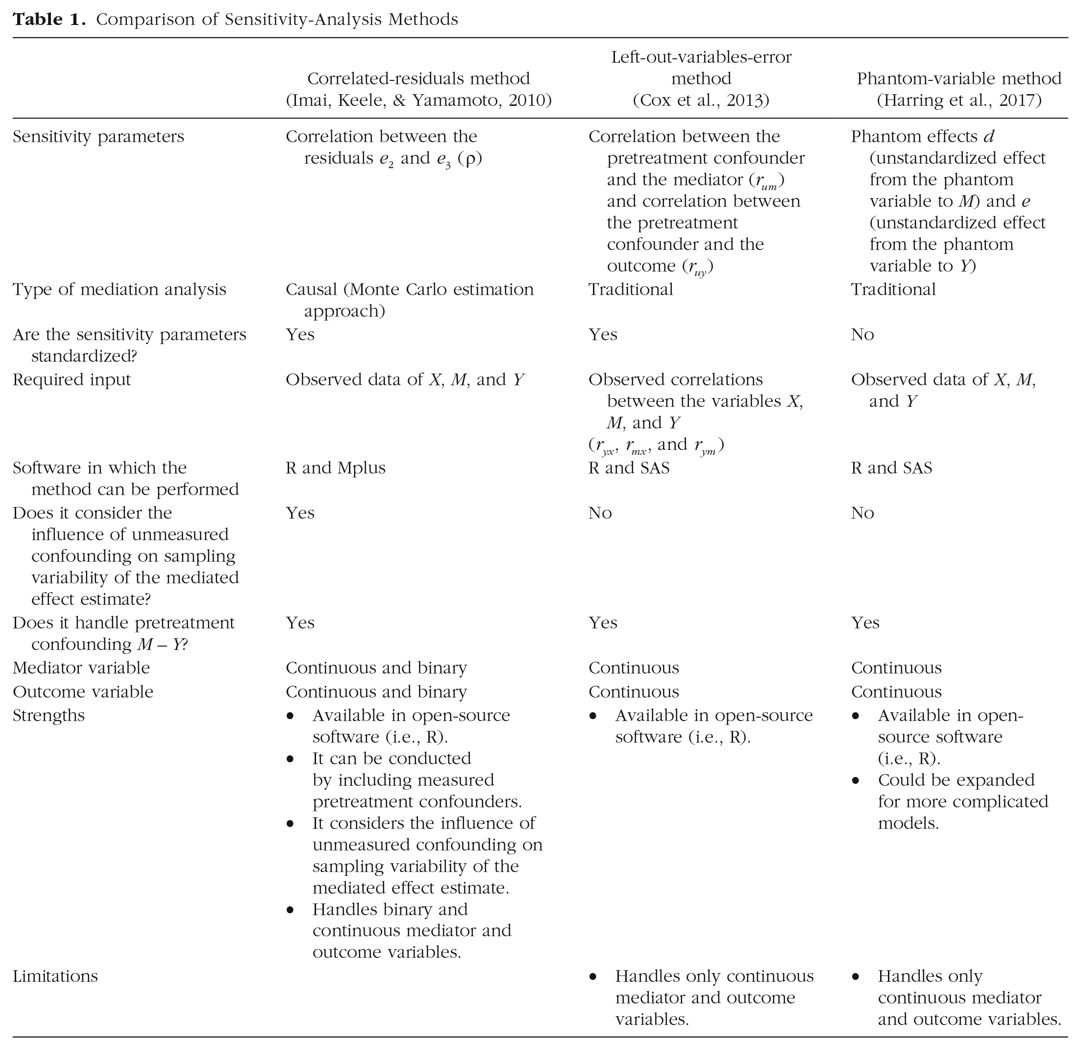
A strength of the correlated-residuals method is that it can be conducted in the widely used R mediation package (Tingley et al., 2014) and in the Mplus software, which allows the user to conduct the mediation analysis including measured pretreatment confounders. Additional programming could develop similar approaches for the LOVE method with the analysis of correlations between the pretreatment confounder with M and Y, adjusted for measured pretreatment confounders. In addition, the phantom-variable model could include additional predictors of M and Y representing measured pretreatment confounders. An additional advantage of the correlated-residuals method is that it considers the influence of unmeasured confounding on sampling variability of the mediated effect estimate, which could be added to the LOVE and phantom-variable methods, but this has not yet been done. Further strengths of the correlated-residuals method are that the current program conducts sensitivity analysis for binary and continuous variables.

Overall, the correlated-residuals method seems to be the method of choice because of the capabilities of the existing program in R, the straightforward inclusion of measured confounders, and extensions to more complicated models, such as models with binary variables. The phantom-variable method’s major strength is that with additional programming, it could apply to more complicated models, such as longitudinal models, in which the influence of confounding of one aspect of the model could be evaluated. Of course, it is assumed that each method operates as expected with data, which will be evaluated in the rest of this article.

In this article, we compare three sensitivity-analysis methods: the correlated-residuals method, the LOVE method, and the phantom-variable method. However, we also note the additional contributions to sensitivity-analysis methods for other scenarios. For instance, VanderWeele (2010) developed a sensitivity analysis derived from the potential-outcomes framework of mediation analysis that focuses on binary confounders. Hong et al. (2018) proposed a sensitivity analysis for causal mediation analysis based on the ratio-of-mediator-probability-weighting method (Hong et al., 2015) that tests the aggregate bias associated with multiple omitted confounders, which could be pretreatment or posttreatment confounder variables. The method developed by Hong et al. (2018) has the flexibility of incorporating interactions between the measured or unmeasured confounders and X or M, and it can be extended to nonexperimental designs (i.e., when X is observed). Qin and Yang (2022) developed a simulation-based sensitivity analysis for causal-mediation studies suitable for continuous and binary mediator and outcome variables and for randomized and observational studies, which is available in the mediationsens R package. McCandless and Somers (2019) proposed a sensitivity analysis that assesses unmeasured confounding bias in mediation analysis using Bayesian methods. In addition, researchers have developed sensitivity analyses that simultaneously test the no-unmeasured-pretreatment-confounding assumption and the no-measurement-error assumption (Fritz et al., 2016; Lin et al., 2023; X. Liu & Wang, 2021). Tofighi et al. (2019) developed a sensitivity analysis that tests unmeasured confounding bias for growth-curve mediation models. Table 2 summarizes the extensions of sensitivity analyses for other situations.

Table 2.

Extensions of Sensitivity Analyses to Test Unmeasured Confounding in Mediation Analysis

Extensions	Reference
Allows examination of unmeasured pretreatment confounding on the X to M and X to Y relations	Hong et al. (2018) Qin and Yang (2022) McCandless and Somers (2019)
Allows examination of unmeasured posttreatment confounding (i.e., an unmeasured confounder on the M to Y relation affected by X)	Hong et al. (2018) Lin et al. (2023)
Derived from the potential-outcome framework of mediation analysis	VanderWeele (2010) Hong et al. (2018) McCandless and Somers (2019) Multiple estimators: Qin and Yang (2022)
Requires including the observed covariates to determine a plausible range of potential bias	Pretreatment/posttreatment observed confounders: Hong et al. (2018) Pretreatment observed confounders: Qin and Yang (2022)
Allows examination of violations to the no-measurement-error assumption	Fritz et al. (2016) Lin et al. (2023) X. Liu and Wang (2021)
Incorporates uncertainty about unmeasured confounding by using prior distributions for sensitivity parameters	McCandless and Somers (2019)
Allows examination of unmeasured confounding in more complex models beyond the single-mediator model	Tofighi et al. (2019)

We selected the correlated-residuals method, LOVE method, and the phantom-variable method in this study to exemplify sensitivity to unmeasured pretreatment confounding in the simplest scenario, a single-mediator model, where X represents random assignment to treatment and control groups, assuming a continuous pretreatment confounder and no interaction between the independent variable and the mediator. Sensitivity analyses in Table 2 have capabilities beyond the focus of this study.

Applied Example

Memory study

We applied three sensitivity-to-unmeasured-pretreatment-confounding methods to a data set from a memory study (MacKinnon et al., 2018). Researchers randomly assigned 44 participants to two conditions: primary and secondary rehearsal groups. A researcher read aloud a list of words, and participants were given specific instructions depending on the group they were assigned to. Participants in the primary rehearsal group were asked to repeat the words they listened to, and participants in the secondary rehearsal group were asked to make mental images of those words. In the end, participants were asked to report the number of words they remembered. In the data set, X represents random assignment to conditions, coded 0 (primary rehearsal) and 1 (secondary rehearsal). The mediator (M) is the response to the question about how much each participant made mental images of the words, scored from 1 (not at all) to 9 (definitely), and Y represents the total number of words that people remembered (out of 20; for data set from the memory study, see Appendix A in the Supplemental Material available online).

Results

The results from the mediation analysis show that the mediated effect from the type of rehearsal (X) to the number of words remembered (Y) through imagery (M) was statistically significant: $a b$ = 2.19, 95% confidence interval (CI) = [0.70, 3.85]. The effect from the type of rehearsal (X) to imagery (M) was statistically significant ( $a$ = 3.56, $z$ = 5.56, $p$ < .001), and the effect from imagery (M) to the total of words remembered (Y) adjusted for X was also statistically significant ( $b$ = 0.61, $z$ = 2.80, $p$ < .01). For the syntax and results from the mediation analyses, conducted in the lavaan R package, see Appendix B in the Supplemental Material.

To evaluate whether the mediated-effect estimate is robust to unmeasured pretreatment confounding, we conducted three sensitivity analyses: the correlated-residuals method, the LOVE method, and the phantom-variable method. We consider the knowledge of mnemonic techniques a possible unobserved pretreatment confounder.

Correlated-residuals method

We conducted the correlated-residuals method (Imai, Keele, & Yamamoto, 2010) in the R environment (R Core Team, 2021) using the mediation package (Tingley et al., 2014), adapting the code provided by Cox et al. (2013). First, we specified the mediator and outcome equations (i.e., Equations 2 and 3, respectively). Then, we used the mediate function to estimate the ACME and their 95% bootstrap CIs (ACME = 2.19, 95% CI = [0.64, 3.74]) and conducted the sensitivity analysis with the sens.out function. Figure 3 shows how the ACME changes as a function of the sensitivity parameter ( $ρ$ ). The results show that the value of $ρ$ that makes the ACME zero in this data set is 0.39, which means that the original conclusion about the direction of the ACME under the sequential-ignorability assumption (represented by the dashed horizontal line) would be maintained unless $ρ$ is higher than 0.39. The result holds even when we account for sampling variability; the CI covers the value of zero only when 0.11 < ρ < 0.58. For the code and output of the correlated-residuals method, see Appendix C in the Supplemental Material.

LOVE method

The LOVE method (Cox et al., 2013; Mauro, 1990) was conducted in the SAS programming language and the R environment (R Core Team, 2021) using the code provided by Cox et al. (2013). To assess unmeasured pretreatment confounding in the M to Y relation in the single-mediator model, the LOVE method uses the estimates of three correlations: (a) the correlation between the outcome and the independent variable $(r_{y x}$ ), (b) the correlation between the mediator and the independent variable $(r_{m x})$ , and (c) the correlation between the outcome and the mediator ( $r_{y m}$ ). The estimates of these correlations⁴ in the memory data set were $r_{y x} = . 34$ , $r_{m x} = . 62$ , $r_{y m} = . 50$ .

The code for this method generates values from 0 to 1 for two unmeasured correlations: (a) the correlation between the unmeasured pretreatment confounder (e.g., knowledge of mnemonic techniques) and the mediator (i.e., imagery; $r_{u m}$ ) and (b) the correlation between the unmeasured pretreatment confounder (e.g., the knowledge of mnemonic techniques) and the outcome variable (i.e., the total of words remembered; r_uy). The correlation between the independent variable and the unmeasured pretreatment confounder ( $r_{x u}$ ) was fixed to zero. Figure 4 shows a plot for all the values of $r_{u y}$ (x-axis) and $r_{u m}$ (y-axis) that make the standardized mediated effect ( $a^{*} b^{*}$ ) zero. At the far left, Figure 4 shows that it would take a correlation between imagery (M) and the unmeasured pretreatment confounder ( $r_{u m}$ ) to be 1 and the correlation between the total number of words remembered (Y) and the pretreatment confounder ( $r_{u y}$ ) to be around .29 to make the standardized mediated effect zero. At the far right, Figure 4 shows that it would take a correlation between imagery (M) and the unmeasured pretreatment confounder ( $r_{u m}$ ) to be around .29 and the correlation between the total number of words remembered (Y) and the pretreatment confounder ( $r_{u y}$ ) to be 1 to make the standardized mediated effect zero.

For the code and output of the LOVE method, see Appendix D in the Supplemental Material. For the code in SAS, see Figure D1 in the Supplemental Material; for the code in R, see Figure D2 in the Supplemental Material.

Phantom-variable method

The phantom-variable sensitivity-analysis method was conducted in the R environment (R Core Team, 2021) using the lavaan package (Rosseel, 2012) following the description in MacKinnon (in press) and adapted from an earlier version of the code used in Georgeson et al. (2023). The phantom variable was specified with the two mediation equations, and its mean and variance were fixed to 0 and 1, respectively. The program varied the effect of the phantom variable on the mediator (phantom variable → M) and the effect of the phantom variable on the outcome variable (phantom variable → Y) and calculated the mediated effect (ab) for each fixed value. Figure 5 shows how the mediated effect (ab) changes as a function of the value of the phantom-variable effects. The sensitivity-analysis results show that the values of the effect of the phantom variable on the mediator and the effect of the phantom variable on the outcome that render the mediated effect (ab) to zero in this data set are −1.74 and 1.74. For the code to perform the phantom-variable sensitivity-analysis method, see Appendix E in the Supplemental Material.

Simulation study

Motivation

The goal of the simulation study was to evaluate whether the correlated-residuals method, the LOVE method, and the phantom-variable method work as expected across a large number of data sets with different effect sizes and sample sizes. We were interested in assessing the pattern of sensitivity-parameter values needed to make the mediated effect zero as the population confounding effect (de) increased and as the population mediated effect increased (ab) and whether the pattern changed as the sample size increased. We expected that the required values of sensitivity parameters to render a mediated effect zero follow the size of the population mediation effect and would be more accurate with larger sample sizes. We wanted to assess the extent to which the size of the confounding effect would influence the results of the sensitivity methods.

Method

Data generation

A Monte Carlo simulation study was conducted using the SAS 9.4 programming language and the R environment (R Core Team, 2021). The data were generated in the SAS 9.4 programming language based on a single-mediator model with a pretreatment confounder (U) causing the mediator (M) and the outcome (Y; Fig. 2), where M, Y, and U were generated as continuous variables and X was generated as a binary variable, representing random assignment to treatment and control groups. Residuals for each variable were generated as normal variates.

The simulation had five sample sizes (N = 50, 100, 200, 500, 1,000) and the following population-parameter values ( $a$ = 0, 0.14, 0.39, 0.59; $b$ = 0, 0.14, 0.39, 0.59; $c$ = 0, 0.14; $d$ = 0, 0.14, 0.39, 0.59; $e$ = 0, 0.14, 0.39, 0.59) for a total of 360 parameter combinations consistent with sample sizes and effect sizes in psychology-research studies. The simulation study had two factors of interest: The first factor was the effect size of the b-path ( $b$ = 0, 0.14, 0.39, 0.59), and the second factor was the magnitude of the population confounding effect, denoted by the product of $d$ times $e$ ( $d e$ = 0, 0.0196, 0.1521, 0.3481). There were 1,000 replications for each condition.

Correlated-residuals method

Each generated data set was analyzed with the single-mediator model (Equations 2 and 3) in the R environment (R Core Team, 2021) using the mediation package (Tingley et al., 2014), which was called from the SAS language programming with the proc iml function. In other words, the analysis omitted the pretreatment confounding variable (U) from the regression equations and did not include the interaction between the independent variable and the mediator (i.e., XM). The correlated-residuals sensitivity-analysis method was conducted using the sens.out function to obtain the sensitivity parameter $ρ$ (i.e., the correlation between residuals e₂ and e₃) needed to make the ACME zero, which was saved for every data set.

LOVE method

The LOVE method (Cox et al., 2013; Mauro, 1990) was conducted in the SAS 9.4 programming language and the R environment (R Core Team, 2021). Three correlations were estimated for each data set: (a) the correlation between the outcome and the independent variable $(r_{y x}$ ), (b) the correlation between the mediator and the independent variable $(r_{m x})$ , and (c) the correlation between the outcome and the mediator ( $r_{y m}$ ). Based on these correlations, the program generated values from 0 to 1 in increments of .001 for the two unobserved correlations ( $r_{u m}$ ) and ( $r_{u y}$ ) and then calculated the estimates of the standardized $b^{*}$ , $c^{*}$ , and $a^{*}$ coefficients using Equations 9 through 11. For each replication, the program selected the values of $r_{u m}$ and $r_{u y}$ that make the standardized mediated ( $a^{*} b^{*}$ ) effect zero. Contrary to the correlated-residuals method, the LOVE method provides a range of values for $r_{u m}$ and $r_{u y}$ . To have one value for each data set, we decided to select the cases in which the two unobserved correlations were equal ( $r_{u m} = r_{u y}$ ), and then we selected and saved the smallest value for each replication.

Phantom-variable method

The phantom-variable method (Harring et al., 2017; Lovis-McMahon & MacKinnon, 2014; MacKinnon, in press) was conducted in the R environment (R Core Team, 2021) using the lavaan package (Rosseel, 2012), which was called from the SAS language programming using the proc iml function. The code was adapted from an earlier version of the code used in Georgeson et al. (2023). We specified the phantom variable in the two mediation equations (Equations 2 and 3). The program varied the effect of the phantom variable on the mediator (phantom variable → M) and the effect of the phantom variable on the outcome variable (phantom variable → Y) from −2 to 2 in increments of .01 and calculated the mediated effect (ab) for each fixed value. The substantive example shows that this sensitivity-analysis method yields two sensitivity-parameter values, each possessing the same magnitude but a different sign. To simplify comparing the results between methods, we saved the absolute value for each replication, resulting in a single sensitivity-parameter value.

Results

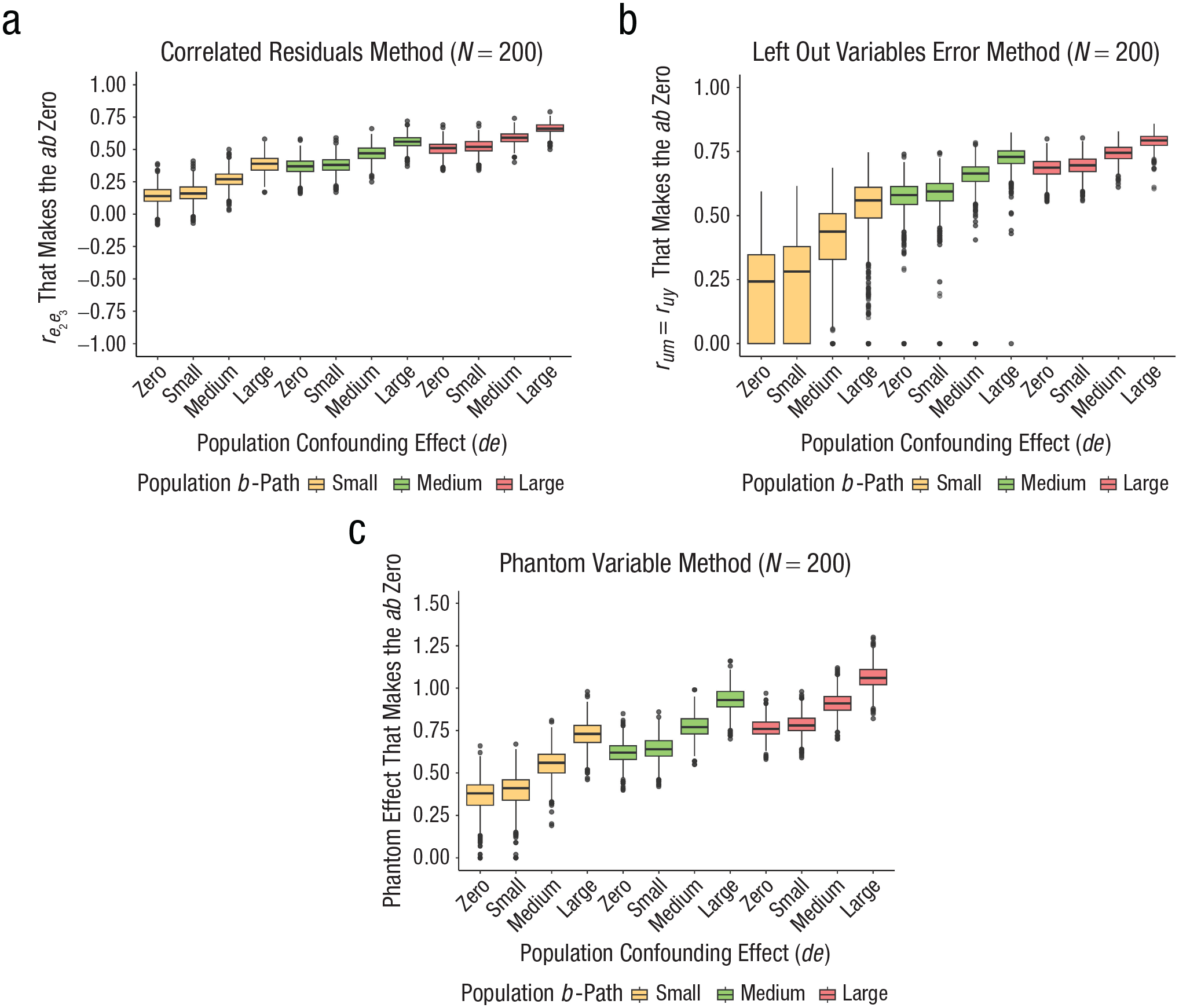
Figures 6 through 8 show the simulation results for the three sensitivity-to-unmeasured-pretreatment-confounding methods: the correlated-residuals method, the LOVE method, and the phantom-variable method for sample size N = 200. The results for other sample sizes (N = 50, 100, 500, 1,000) followed the same pattern (see Appendix G in the Supplemental Material).

Fig. 6.

Average sensitivity-parameter values that make the mediated effect (ab) zero as a function of the population confounding effect (de), the population a-path, and the population b-path (a = nonzero, b = 0, N = 200). (a) Correlated-residuals method. (b) Left-out-variables-error method. (c) Phantom-variable method. The population confounding effect (de) is shown in the x-axis (zero = 0, small = 0.0196, medium = 0.1521, large = 0.3481). Results are shown for conditions in which the population b-path is zero (blue = zero = 0). The average values of the sensitivity-parameter values that make the mediated effect zero are shown on the y-axis.

Fig. 7.

Average sensitivity-parameter values that make the mediated effect (ab) zero as a function of the population confounding effect (de), the population a-path, and the population b-path (a = 0, b = nonzero, N = 200). (a) Correlated-residuals method. (b) Left-out-variables-error method. (c) Phantom-variable method. The population confounding effect (de) is shown in the x-axis (zero = 0, small = 0.0196, medium = 0.1521, large = 0.3481). The population b-path is shown with different colors (blue = zero = 0, yellow = small = 0.14, green = medium = 0.39, pink = large = 0.59). The average values of the sensitivity-parameter values that make the mediated effect zero are shown on the y-axis.

Fig. 8.

Average sensitivity-parameter values that make the mediated effect (ab) zero as a function of the population confounding effect (de), the population a-path, and the population b-path (a = nonzero, b = nonzero, N = 200). (a) Correlated-residuals method. (b) Left-out-variables-error method. (c) Phantom-variable method. The population confounding effect (de) is shown in the x-axis (zero = 0, small = 0.0196, medium = 0.1521, large = 0.3481). The population b-path is shown with different colors (blue = zero = 0, yellow = small = 0.14, green = medium = 0.39, pink = large = 0.59). The average values of the sensitivity-parameter values that make the mediated effect zero are shown on the y-axis.

Figures 6 through 8 show how the sensitivity parameters (shown in the y-axis) change as a function of different combinations of the population confounding effect (de) and the population b- and a-paths. The population confounding effect (de) is shown on the x-axis, where zero = 0, small = 0.0196, medium = 0.1521, and large = 0.3481. The population b-path is portrayed with different colors (blue = zero = 0, yellow = small = 0.14, green = medium = 0.39, pink = large = 0.59).

The sensitivity parameter for the correlated-residuals method is the $ρ$ value (i.e., the correlation between residuals e₂ and e₃) needed to make the mediated effect zero ( $a b = 0$ ). The sensitivity parameter for the LOVE method is the smallest value where these correlation values are equal ( $r_{u m}$ = $r_{u y}$ ) that is needed to make the standardized mediated effect zero ( $a^{*} b^{*} = 0$ ). Finally, the sensitivity parameter for the phantom-variable method is the absolute value of the phantom effects (phantom variable → M) and (phantom variable → Y) that make the mediated effect zero ( $a b = 0$ ).

Figures 6 and 7 show the results for conditions in which the population mediated effect is zero (ab = 0). For these conditions, we expect that across samples from this population, a very small sensitivity parameter is sufficient for removing a mediated effect estimate in the sample if the population value of the mediated effect is zero. We assessed the results for the case when the population mediated effect was zero because the idea of this study was to conduct the sensitivity analyses using the mediated-effect-sample estimates when the researcher does not know the population value. In other words, the population mediated effects were zero; however, the mediated effect estimates will not be always exactly zero in the sample.

As shown in Figure 6, for conditions in which the population a-path is nonzero (small = 0.14, medium = 0.39, large = 0.59) and the population b-path is zero (b = 0), the results show that as the population confounding effect (de) increases, the mean of the sensitivity parameters, leading to a zero-mediated effect, also increases. The sensitivity-parameter results suggest that the sample mediated effect may be considered unaffected by confounding when there is a population zero mediated effect but confounding (de) is present. The pattern of results is consistent for the three sensitivity methods and shows some conflation of the mediated and confounding effects.

Figure 7 shows the results for conditions in which the population a-path is zero (a = 0) and the population b-path is nonzero. As the effect size of the population b-path increases (yellow = small = 0.14, green = medium = 0.39, pink = large = 0.59), the average sensitivity parameter that leads to a zero mediated effect also increases. In other words, as the effect size of the population b-path gets larger, the sensitivity analyses will suggest that the estimated mediated effect is less affected by unmeasured confounding. As in Figure 6, the results show that as the population confounding effect (de) increases, within each size of the population b-path, the mean of the sensitivity parameter that leads to a zero mediated effect also increases. There is a difference in the LOVE results compared with the other methods when the a-path is zero; the values of $r_{u m}$ and $r_{u y}$ needed to make the standardized mediated effect zero are in a very wide range for all the sizes of the population b-path. The values of the sensitivity parameters from the correlated-residuals method and the phantom-variable method reflect the population b-path instead of the population mediated effect.

Figure 8 shows the results for conditions in which the population mediated effect is nonzero (ab ≠ 0). For these conditions, we expect that the sensitivity parameters needed to make the mediated effect zero reflect the population mediated effect. As expected, as the effect size of the population b-path increases, the average sensitivity parameter that leads to a zero mediated effect also increases. And as the population confounding effect (de) increases, within each size of the population b-path, the mean of the sensitivity parameter that leads to a zero mediated effect also increases, showing some conflation of the population mediated and confounding effects.

Finally, results show that the variability of the average sensitivity-parameter values decreases as the sample size increases (for results for all sample sizes, see Appendix G in the Supplemental Material). In other words, the larger the sample size is, the smaller the range of the values of the sensitivity parameter that make the mediated effect zero is. The results are consistent across methods, except for the LOVE method, when the population a-path is zero, which has more variability in the sensitivity-parameter value that renders the standardized mediated effect zero.

A limitation of the LOVE method as used in this study was that it did not provide a sensitivity-parameter value for all the replications because of the way that the values of the unmeasured correlations $r_{u m}$ and $r_{u y}$ were selected. In some generated data sets, there were no instances in which the unmeasured correlations were equal (i.e., $r_{u m}$ = $r_{u y}$ ). For the frequency of data sets with a sensitivity parameter for the LOVE method for each parameter combination, see Appendix F in the Supplemental Material.

Discussion

Unmeasured confounding threatens the causal interpretation of the mediated effect estimates. Sensitivity analyses help deal with confounding bias in mediation analysis when potential confounders are not measured in the study. Lee et al. (2021) proposed guidelines for reporting mediation analyses of randomized trials and observational studies. They suggested that researchers routinely report sensitivity analyses used to explore the causal assumptions, including assumptions about confounding. These methods are recommended in the single-mediator model and more complex models (Tofighi et al., 2019), but the different sensitivity-to-confounding methods have not been compared. Our present research work was motivated by recommendations to investigate confounding in mediation analysis and the high probability of unmeasured confounders of the M to Y relation in most studies. It is important to evaluate how sensitivity-analysis methods to test unmeasured confounding work if researchers are encouraged to use and report them regularly.

The results are consistent across methods, showing that the effect size of the population b-path and the magnitude of the population confounding effect (de) determined the smallest size of the sensitivity parameters that make the mediated effect zero. There was a larger shift in the sensitivity parameter resulting from the b-path than the modest shifts in the sensitivity parameter from the confounding effect size (de). Overall, the results indicate that one method to assess sensitivity to unmeasured confounder bias is to evaluate the effect size of the b-path. If the b-path is large, confounder bias is less likely to render an observed mediated effect equal to zero. The critical role of the magnitude of the b-path for sensitivity to confounding in mediation analysis is consistent with Hill’s (1965) first consideration for a causal relation, which emphasizes the strength of the effect as evidence that the effect is causal, such as “strong associations are more likely to be causal than weak associations because, if they could be explained by some other factor, the effect of that factor would have to be even stronger than the observed association” (Rothman & Greenland, 2005, p. S148). That recommendation also applies to sensitivity to confounding in mediation analysis. A large b-path effect protects from unmeasured confounding because confounder effects would have to be larger to explain the observed large b-path.

There are some caveats about focusing sensitivity to confounding on the b-path. First, for mediation to exist, there must be evidence that X causes M. If X does not cause M, then there will not be mediation despite the size of the b-path. Second, there are other spurious influences that inflate the M to Y path, such as measurement overlap (i.e., using similar individual items for measuring M and Y), selection of the sample by a collider that alters the relation between M and Y, or more complicated models with additional mediators and confounders that may alter the relation between M and Y. Nevertheless, consideration of confounding of the M to Y path, including consideration of the size of the b-path, in experimental mediation analysis provides one way to evaluate sensitivity to unmeasured confounder bias.

General Recommendations for Substantive Researchers

In this section, we include general recommendations based on the existing literature and the current study’s results to improve the causal interpretation of the mediated effect.

First, whenever possible, we recommend that substantive researchers use design-based techniques (in which both the independent variable and the mediator are randomized) to enhance a causal interpretation of the mediated effect (e.g., sequential double-randomization design, concurrent double-randomization design, and parallel randomization). For a detailed description of these designs, see Pirlott and MacKinnon (2016).

Second, if randomly assigning participants to both the independent variable and the mediator is not possible, as is often the case, we encourage researchers to think about the potential confounders of their specific variables before conducting the study, measure the confounders at baseline, and adjust for them during the analysis. A variety of methods are available for adjusting for measured confounders, including analysis of covariance and weighting approaches (for an explanation of other statistical techniques to incorporate measures of confounding variables, see MacKinnon & Pirlott, 2015; Shadish et al., 2008; Valente et al., 2017). Overall, it is recommended that researchers carefully select and justify, both theoretically and empirically, each pretreatment covariate in the model (Simmons et al., 2011; Wysocki et al., 2022).

Third, if the independent variable was randomized but the mediating variable was not, we recommend using a sensitivity-analysis method described in this article to assess how robust the mediated effect is to unmeasured pretreatment confounding bias. We also recommend looking at the effect size of the b-path as an important first step in these analyses. The interpretation of the unmeasured pretreatment confounder effect sizes may depend on the area of research and should be interpreted considering the effect sizes typically observed in the research area.

Fourth, several reasons make the correlated-residuals method the overall method of choice for assessing sensitivity to unmeasured pretreatment confounding on the M to Y relation. The correlated-residuals method can be conducted in R and Mplus, easily incorporates measured confounders as predictors, can handle binary and continuous variables, and generates information about how unmeasured pretreatment confounding affects the sampling variability of the observed mediated effect. If a large structural equation model is part of the research project, then the phantom-variable method is ideal because the sensitivity to confounding could be included as part of larger models.

Limitations and Future Directions

The current study has some limitations, and in this section, we make suggestions for future research. First, in the present research, we focused on assessing the sensitivity of unmeasured pretreatment confounding in the M to Y relation (b-path) for the common experimental application of mediation analysis for continuous M and Y. However, future research could compare sensitivity-analysis methods that are suitable to test unmeasured pretreatment confounding of the X to M and X to Y relations when X is nonrandomized (e.g., Hong et al., 2018; Qin & Yang, 2022).

Second, in the present study, we focused on data with a continuous mediator and a continuous outcome variable. Future research could compare sensitivity-analysis methods that were developed to test unmeasured confounding when the mediator or/and the outcome variables are binary (e.g., Imai, Keele, & Yamamoto, 2010; Qin & Yang, 2022). Binary mediators or outcomes are frequently encountered in mediation analysis. Common examples in health-related research include variables such as health status (e.g., healthy vs. unhealthy), medical test results (e.g., positive vs. negative), smoking status (e.g., smoker vs. nonsmoker), and mortality (e.g., alive vs. deceased; Xu et al., 2023). The same issues discussed in this article will apply to binary variables, including the importance of measuring confounders and the evaluation of sensitivity to confounding by varying the strength of the relation of unmeasured confounders to M and Y.

Third, in the present research, we focused on comparing sensitivity-analysis methods while assuming that the mediator has been measured without error. Future research could compare sensitivity-analysis methods that test multiple assumptions simultaneously (e.g., Fritz et al., 2016; Lin et al., 2023; X. Liu & Wang, 2021).

Fourth, in the current study, we generated data for a zero value of the interaction between the independent variable (X) and the mediator (M; i.e., g = 0), as is commonly assumed in experimental mediation studies. A future study could generate data violating this assumption and assess how the sensitivity-analysis methods included in the present study perform compared with methods that incorporate the XM interaction (e.g., Hong et al., 2018; Imai, Keele, & Yamamoto, 2010; Qin & Yang, 2022). When there is an XM interaction, the mediated effect has several definitions, including the PNIE and the TNIE, as described in Valeri and VanderWeele (2013). The sensitivity analyses then focus on the size of confounder relations that reduce the PNIE and the TNIE equal to zero.

In conclusion, inference from statistical-mediation analysis relies on several assumptions, including no unmeasured M to Y confounding. Three methods to assess sensitivity to unmeasured pretreatment confounding of M to Y were clarified by their application to a real data set and in a large statistical simulation study. Overall, the different methods performed similarly such that larger effect sizes of the population b-path (and corresponding sample b-path) make the mediated effect estimates less affected by confounding bias. One recommendation for researchers investigating confounding bias in the M to Y relation in the single-mediator model when X is randomized but M is not is to assess the effect size of the path relating M to Y (b-path). More details about the role of confounding can be obtained by conducting one or more of the sensitivity-analysis methods in this article. At this time, the correlated-residuals method is the easiest to use and has the most capabilities.

Supplemental Material

sj-docx-1-amp-10.1177_25152459251355586 – Supplemental material for Three Sensitivity-Analysis Methods to Assess Unmeasured Pretreatment Confounding Bias in Experimental Mediation Analysis

Supplemental material, sj-docx-1-amp-10.1177_25152459251355586 for Three Sensitivity-Analysis Methods to Assess Unmeasured Pretreatment Confounding Bias in Experimental Mediation Analysis by Diana Alvarez-Bartolo and David P. MacKinnon in Advances in Methods and Practices in Psychological Science

Footnotes

Transparency

Action Editor: Rogier Kievit

Editor: David A. Sbarra

Author Contributions

Diana Alvarez-Bartolo: Conceptualization; Data curation; Formal analysis; Investigation; Methodology; Software; Validation; Visualization; Writing – original draft.

David P. MacKinnon: Conceptualization; Funding acquisition; Investigation; Methodology; Project administration; Resources; Supervision; Writing – review & editing.

ORCID iDs

Diana Alvarez-Bartolo

David P. MacKinnon

Supplemental Material

Additional supporting information can be found at .

Notes

References

Baron

R. M.

Kenny

D. A.

(1986). The moderator–mediator variable distinction in social psychological research: Conceptual, strategic, and statistical considerations. Journal of Personality and Social Psychology, 51(6), 1173–1182. https://doi.org/10.1037/0022-3514.51.6.1173

Coffman

D. L.

Schuler

M. S.

Nguyen

T. Q.

McCaffrey

D. F.

(2023). Weighting estimators for causal mediation. In Zubizaretta

H. R.

Stuart

E. A.

Small

D. S.

Rosenbaum

P. R.

(Eds.), Handbook of matching and weighting adjustments for causal inference (pp. 373–412). Chapman and Hall.

Cole

D. A.

Maxwell

S. E.

(2003). Testing mediational models with longitudinal data: Questions and tips in the use of structural equation modeling. Journal of Abnormal Psychology, 112(4), 558–577. https://doi.org/10.1207/S15328007SEM1002_5

Cornfield

Haenszel

Hammond

E. C.

Lilienfeld

A. M.

Michael

B. S.

Ernst

L. W

. (1959). Smoking and lung cancer: Recent evidence and a discussion of some questions. Journal of the National Cancer Institute, 22(1), 173–203. https://doi.org/10.1093/jnci/22.1.173

Cox

M. G.

Kisbu-Sakarya

Miocˇević

MacKinnon

D. P.

(2013). Sensitivity plots for confounder bias in the single mediator model. Evaluation Review, 37(5), 405–431. https://doi.org/10.1177/0193841X14524576

Frank

K. A.

(2000). Impact of a confounding variable on a regression coefficient. Sociological Methods & Research, 29(2), 147–194. https://doi.org/10.1177/0049124100029002001

Frank

K. A.

Lin

Maroulis

Mueller

(2023). Quantifying the robustness of causal inferences: Sensitivity analysis for pragmatic social science. Social Science Research, 110, Article 102815. https://doi.org/10.1016/j.ssresearch.2022.102815

Frank

K. A.

Maroulis

S. J.

Duong

M. Q.

Kelcey

B. M.

(2013). What would it take to change an inference? Using Rubin’s causal model to interpret the robustness of causal inferences. Educational Evaluation and Policy Analysis, 35(4), 437–460. https://doi.org/10.3102/0162373713493129

Fritz

M. S.

Kenny

D. A.

MacKinnon

D. P.

(2016). The combined effects of measurement error and omitting confounders in the single-mediator model. Multivariate Behavioral Research, 51(5), 681–697. https://doi.org/10.1080/00273171.2016.1224154

10.

Georgeson

A. R.

Alvarez-Bartolo

MacKinnon

D. P.

(2023). A sensitivity analysis for temporal bias in cross-sectional mediation. Psychological Methods. Advance online publication. https://doi.org/10.1037/met0000628

11.

Gonzalez

MacKinnon

D. P.

(2021). The measurement of the mediator and its influence on statistical mediation conclusions. Psychological Methods, 26(1), 1–17. https://doi.org/10.1037/met0000263

12.

Harring

J. R.

McNeish

D. M.

Hancock

G. R.

(2017). Using phantom variables in structural equation modeling to assess model sensitivity to external misspecification. Psychological Methods, 22(4), 616–631. https://doi.org/10.1037/met0000103

13.

Hill

A. B.

(1965). The environment and disease: Association or causation? Proceedings of the Royal Society of Medicine, 58(5), 295–300. https://doi.org/10.1177/003591576505800503

14.

Holland

P. W.

(1986). Statistics and causal inference. Journal of the American Statistical Association, 81(396), 945–960. https://doi.org/10.2307/2289064

15.

Hong

Deutsch

Hill

H. D.

(2015). Ratio-of-mediator-probability weighting for causal mediation analysis in the presence of treatment-by-mediator interaction. Journal of Educational and Behavioral Statistics, 40(3), 307–340. https://doi.org/10.3102/1076998615583902

16.

Hong

Qin

Yang

(2018). Weighting-based sensitivity analysis in causal mediation studies. Journal of Educational and Behavioral Statistics, 43(1), 32–56. https://doi.org/10.3102/1076998617749561

17.

Imai

Keele

Tingley

(2010). A general approach to causal mediation analysis. Psychological Methods, 15(4), 309–334. https://doi.org/10.1037/a0020761

18.

Imai

Keele

Yamamoto

(2010). Identification, inference and sensitivity analysis for causal mediation effects. Statistical Science, 25(1), 51–71. https://doi.org/10.1214/10-STS321

19.

James

L. R.

(1980). The unmeasured variables problem in path analysis. Journal of Applied Psychology, 65(4), 415–421. https://doi.org/10.1037/0021-9010.65.4.415

20.

Lee

Cashin

A. G.

Lamb

S. E.

Hopewell

Vansteelandt

VanderWeele

T. J.

MacKinnon

D. P.

Mansell

Collins

G. S.

Golub

R. M.

(2021). A guideline for reporting mediation analyses of randomized trials and observational studies: The AGReMA statement. JAMA, 326(11), 1045–1056. https://doi.org/10.1001/jama.2021.14075

21.

Lin

Nuttall

A. K.

Zhang

Frank

K. A.

(2023). How do unobserved confounding mediators and measurement error impact estimated mediation effects and corresponding statistical inferences? Introducing the R package ConMed for sensitivity analysis. Psychological Methods, 28(2), 339–358. https://doi.org/10.1037/met0000567

22.

Liu

Kuramoto

S. J.

Stuart

E. A.

(2013). An introduction to sensitivity analysis for unobserved confounding in nonexperimental prevention research. Prevention Science, 14(6), 570–580. https://doi.org/10.1007/s11121-012-0339-5

23.

Liu

Wang

(2021). The impact of measurement error and omitting confounders on statistical inference of mediation effects and tools for sensitivity analysis. Psychological Methods, 26(3), 327–342. https://doi.org/10.1037/met0000345

24.

Lovis-McMahon

D. A.

MacKinnon

D. P.

(2014, May 28). Confoundit: Assessing the impact of confounders on mediation [Poster presentation]. 22nd Annual Meeting of the Society for Prevention Research, Washington, DC.

25.

MacKinnon

D. P.

(2008). Introduction to statistical mediation analysis. Routledge.

26.

MacKinnon

D. P.

(in press). Introduction to statistical mediation analysis (2nd ed.). Taylor and Francis.

27.

MacKinnon

D. P.

Pirlott

A. G.

(2015). Statistical approaches for enhancing causal interpretation of the M to Y relation in mediation analysis. Personality and Social Psychology Review, 19(1), 30–43. https://doi.org/10.1177/1088868314542878

28.

MacKinnon

D. P.

Valente

M. J.

Gonzalez

(2020). The correspondence between causal and traditional mediation analysis: The link is the mediator by treatment interaction. Prevention Science, 21, 147–157. https://doi.org/10.1007/s11121-019-01076-4

29.

MacKinnon

D. P.

Valente

M. J.

Wurpts

I. C.

(2018). Benchmark validation of statistical models: Application to mediation analysis of imagery and memory. Psychological Methods, 23(4), 654–671. https://doi.org/10.1037/met0000174

30.

Mauro

(1990). Understanding LOVE (left out variables error): A method for estimating the effects of omitted variables. Psychological Bulletin, 108(2), 314–329. https://doi.org/10.1037/0033-2909.108.2.314

31.

McCandless

L. C.

Somers

J. M.

(2019). Bayesian sensitivity analysis for unmeasured confounding in causal mediation analysis. Statistical Methods in Medical Research, 28(2), 515–531. https://doi.org/10.1177/0962280217729844

32.

Muthén

L. K.

Muthén

B. O.

(2012). Mplus (Version 7.2) [Computer software].

33.

Nguyen

T. Q.

Schmid

Stuart

E. A.

(2021). Clarifying causal mediation analysis for the applied researcher: Defining effects based on what we want to learn. Psychological Methods, 26(2), 255–271. https://doi.org/10.1037/met0000299

34.

Pearl

(2001). Direct and indirect effects. In Proceedings of the Seventeenth Conference on Uncertainty in Artificial Intelligence (pp. 411–420). Association for Computing Machinery.

35.

Pirlott

A. G.

MacKinnon

D. P.

(2016). Design approaches to experimental mediation. Journal of Experimental Social Psychology, 66, 29–38. https://doi.org/10.1016/j.jesp.2015.09.012

36.

Qin

Yang

(2022). Simulation-based sensitivity analysis for causal mediation studies. Psychological Methods, 27(6), 1000–1013. https://doi.org/10.1037/met0000340

37.

R Core Team. (2021). R: A language and environment for statistical computing [Computer software]. R Foundation for Statistical Computing. https://www.R-project.org/

38.

Rijnhart

J. J. M.

Lamp

S. J.

Valente

M. J.

MacKinnon

D. P.

Twisk

J. W. R.

Heymans

M. W.

(2021). Mediation analysis methods used in observational research: A scoping review and recommendations. BMC Medical Research Methodology, 21(1), Article 226. https://doi.org/10.1186/s12874-021-01426-3

39.

Rindskopf

(1984). Using phantom and imaginary latent variables to parameterize constraints in linear structural models. Psychometrika, 49(1), 37–47. https://doi.org/10.1007/BF02294204

40.

Robins

J. M.

Greenland

(1992). Identifiability and exchangeability for direct and indirect effects. Epidemiology, 3(2), 143–155. http://www.jstor.org/stable/3702894

41.

Rohrer

J. M.

(2018). Thinking clearly about correlations and causation: Graphical causal models for observational data. Advances in Methods and Practices in Psychological Science, 1(1), 27–42. https://doi.org/10.1177/2515245917745629

42.

Rosenbaum

P. R.

(2005). Sensitivity analysis in observational studies. In Everitt

B. S.

Howell

D. C.

(Eds.), Encyclopedia of statistics in behavioral science (Vol. 4, pp. 1809–1814). John Wiley & Sons.

43.

Rosseel

(2012). lavaan: An R package for structural equation modeling. Journal of Statistical Software, 48(2), 1–36. https://doi.org/10.18637/jss.v048.i02

44.

Rothman

K. J.

Greenland

(2005). Causation and causal inference in epidemiology. American Journal of Public Health, 95(S1), S144–S150. https://doi.org/10.2105/AJPH.2004.059204

45.

Rubin

D. B.

(1974). Estimating causal effects of treatments in randomized and nonrandomized studies. Journal of Educational Psychology, 66(5), 688–701. https://doi.org/10.1037/h0037350

46.

Sanders

M. R.

Mazzucchelli

T. G.

(2022). Mechanisms of change in population-based parenting interventions for children and adolescents. Journal of Clinical Child & Adolescent Psychology, 51(3), 277–294. https://doi.org/10.1080/15374416.2022.2025598

47.

Shadish

W. R.

Clark

M. H.

Steiner

P. M.

(2008). Can nonrandomized experiments yield accurate answers? A randomized experiment comparing random and nonrandom assignments. Journal of the American Statistical Association, 103(484), 1334–1344. https://doi.org/10.1198/016214508000000733

48.

Simmons

J. P.

Nelson

L. D.

Simonsohn

(2011). False-positive psychology: Undisclosed flexibility in data collection and analysis allows presenting anything as significant. Psychological Science, 22(11), 1359–1366. https://doi.org/10.1177/0956797611417632

49.

Spencer

S. J.

Zanna

M. P.

Fong

G. T.

(2005). Establishing a causal chain: Why experiments are often more effective than mediational analyses in examining psychological processes. Journal of Personality and Social Psychology, 89(6), 845–851. https://doi.org/10.1037/0022-3514.89.6.845

50.

Stuart

E. A.

Schmid

Nguyen

Sarker

Pittman

Benke

Rudolph

Badillo-Goicoechea

Leoutsakos

J.-M.

(2021). Assumptions not often assessed or satisfied in published mediation analyses in psychology and psychiatry. Epidemiologic Reviews, 43(1), 48–52. https://doi.org/10.1093/epirev/mxab007

51.

Tingley

Yamamoto

Hirose

Keele

Imai

(2014). Mediation: R package for causal mediation analysis. Journal of Statistical Software, 59(1), 1–38. https://doi.org/10.18637/jss.v059.i05

52.

Tofighi

Hsiao

Y.-Y.

Kruger

E. S.

MacKinnon

D. P.

Lee Van Horn

Witkiewitz

(2019). Sensitivity analysis of the no-omitted confounder assumption in latent growth curve mediation models. Structural Equation Modeling: A Multidisciplinary Journal, 26(1), 94–109. https://doi.org/10.1080/10705511.2018.1506925

53.

Valente

M. J.

Pelham

W. E.

III Smyth

MacKinnon

D. P.

(2017). Confounding in statistical mediation analysis: What it is and how to address it. Journal of Counseling Psychology, 64(6), 659–671. https://doi.org/10.1037/cou0000242

54.

Valeri

VanderWeele

T. J.

(2013). Mediation analysis allowing for exposure–mediator interactions and causal interpretation: Theoretical assumptions and implementation with SAS and SPSS macros. Psychological Methods, 18(2), 137–150. https://doi.org/10.1037/a0031034

55.

VanderWeele

T. J.

(2010). Bias formulas for sensitivity analysis for direct and indirect effects. Epidemiology, 21(4), 540–551. https://doi.org/10.1097/EDE.0b013e3181df191c

56.

VanderWeele

T. J.

(2016). Mediation analysis: A practitioner’s guide. Annual Review of Public Health, 37, 17–32. https://doi.org/10.1146/annurev-publhealth-032315-021402

57.

VanderWeele

T. J.

Ding

(2017). Sensitivity analysis in observational research: Introducing the e-value. Annals of Internal Medicine, 167(4), 268–274. https://doi.org/10.7326/M16-2607

58.

VanderWeele

T. J.

Vansteelandt

(2009). Conceptual issues concerning mediation, interventions and composition. Statistics and Its Interface, 2(4), 457–468. https://doi.org/10.4310/SII.2009.v2.n4.a7

59.

Witkiewitz

Pfund

R. A.

Tucker

J. A.

(2022). Mechanisms of behavior change in substance use disorder with and without formal treatment. Annual Review of Clinical Psychology, 18, 497–525. https://doi.org/10.1146/annurev-clinpsy-072720-014802

60.

Wysocki

A. C.

Lawson

K. M.

Rhemtulla

(2022). Statistical control requires causal justification. Advances in Methods and Practices in Psychological Science, 5(2). https://doi.org/10.1177/25152459221095823

61.

Coffman

D. L.

Luta

Niaura

R. S.

(2023). Tutorial on causal mediation analysis with binary variables: An application to health psychology research. Health Psychology, 42(11), 778–787. https://doi.org/10.1037/hea0001299

Supplementary Material

Please find the following supplemental material available below.

For Open Access articles published under a Creative Commons License, all supplemental material carries the same license as the article it is associated with.

For non-Open Access articles published, all supplemental material carries a non-exclusive license, and permission requests for re-use of supplemental material or any part of supplemental material shall be sent directly to the copyright owner as specified in the copyright notice associated with the article.

0.00 MB

1.05 MB