
Abstract
Psychological researchers are interested in how things change over time and routinely make claims about age effects (e.g., personality maturation), cohort effects (e.g., generational differences in narcissism), and sometimes, period effects (e.g., secular trends in mental health). The age-period-cohort identification problem means that these claims are not possible based on the data alone: Any possible temporal pattern can be explained by an infinite number of combinations of age, period, and cohort effects. This concern holds regardless of the study design (it also applies to longitudinal designs covering multiple cohorts) and the number of observations available (it also applies if researchers observe the whole population). Researchers usually rely on statistical models that impose constraints to pick one specific decomposition of effects. Unfortunately, these constraints often remain opaque, resulting in a lack of scrutiny of the underlying assumptions. How can researchers reason more transparently and systematically about age, period, and cohort? Here, I summarize advances in the understanding of the precise nature of the identification problem, provide an overview of ways to move forward, and highlight one approach that is particularly transparent about assumptions: bounding analysis, a framework developed by sociologists Ethan Fosse and Christopher Winship. To illustrate this approach, I analyze how age, period, and cohort affect attitudes toward working mothers in the German General Social Survey.
Psychologists are interested in how things change over time. Does personality change for the better as people mature with age? Have modern times made people lonelier than they used to be? Have more recently born cohorts been pampered so much that they have become narcissistic? These are interesting research questions about how people’s age, the period in which they live, and the cohort into which they were born affect important outcomes. However, the age-period-cohort identification problem makes it challenging to actually estimate the corresponding age, period, and cohort effects (for a discussion of the causal status of these effects, see Box 1). This problem has been known and discussed for a long time—already in the 1870s, sophisticated diagrams and basic equations were worked out (Keiding, 2011); debates are still ongoing today. Maybe most notable to psychologists was the Schaie-Baltes controversy (summarized by both parties in Schaie & Baltes, 1975), which hinged on the distinction between description versus explanation (see Box 1) but also on the question concerning the appropriate research design and data analysis (see rest of this article)—all concerns that remain relevant to psychological researchers today.
What Are Age, Period, and Cohort Effects Anyway?

The bad news is that the age-period-cohort problem is as intractable as it was 150 years ago. The good news is that there have been fairly recent advances that allow researchers to reason about it more clearly and more transparently. The goal of this article is to provide an up-to-date introduction to the problem, give an overview of different ways to move forward, and illustrate one particular approach in which assumptions take center stage.
Setting the Stage
The age-period-cohort identification arises because the three variables are in a deterministic relationship: Age equals period minus cohort. For example, somebody who is 35 years old (age = 35) in the year 2025 (period = 2025) was born in 1990 (cohort = 1990 or 1989, depending on the precise date). Because of this relationship, it is impossible to simultaneously estimate age, period, and cohort effects in, for example, a standard linear regression model: There will be perfect multicollinearity. This means that there will always be an infinite number of combinations of age-, period-, and cohort-effect estimates that match the data equally well.
The age-period-cohort problem is not just a statistical estimation issue; in fact, discussing it in statistical terms obscures how fundamental it is. The age-period-cohort problem means that the data can never tell to which extent differences associated with time should be attributed to age, period, or cohort. Now imagine that you are a personality researcher who wants to investigate how age affects personality. You may not be interested in period or cohort effects at all; you do not even consider including all three variables in your analysis. But the age-period-cohort problem still applies. In this particular instance, period and cohort effects on personality may exist. And if they do exist, at least one of them will inevitably be mixed up with the age effects of interest. For this reason, you may underestimate or overestimate how much personality changes with age or even get the sign of the age effect wrong, thus ending up with wrong substantive conclusions.
Data, Design, and Statistics Cannot Solve the Age-Period-Cohort Problem
The age-period-cohort problem is not a problem of statistical inference but, rather, a so-called identification problem. This means that it cannot be solved by simply collecting a larger sample (Fosse & Winship, 2019b; Manski, 2003). It would still apply if the data included the whole population of interest. It also cannot be solved through study design—most importantly, it also applies to studies in which multiple cohorts were followed longitudinally. This may come as a surprise because longitudinal data are often thought to overcome the central shortcomings of cross-sectional data. Longitudinal data certainly have their advantages (e.g., when it comes to other problems of causal inference; Rohrer & Murayama, 2023), but they cannot overcome the identification problem. To understand why, consider two common research designs and how exactly the problem affects them.
Common designs
Cross-sectional data
In the simplest scenario, imagine you have only a single wave of cross-sectional data. Assume that you are interested in the age effects. Period effects are, by design, a nonissue: Everybody in your data was observed in the same period. Thus, you cannot make statements about period effects, and you do not need to worry about them as confounders. What you do need to worry about is that age and cohort are perfectly correlated: In your data, a person who is 1 year older than another person was born precisely 1 year earlier. Thus, if the outcome variable of interest (e.g., some personality trait) is correlated with age, it is necessarily also correlated with cohort. If a person who is 1 year older tends to score 1 point higher in conscientiousness, then a person who was born 1 year earlier tends to score 1 point higher in conscientiousness—in cross-sectional data, these statements are equivalent. As a result, it is unclear whether the differences in conscientiousness should be attributed to age, cohort, or a combination of both.
If at this point you were willing to assume that cohort effects on the outcome simply do not exist, you could move on and interpret your findings: Without cohort effects, the differences you observe should be age effects. 1 Alternatively, you may assume that age effects do not exist and subsequently interpret any observed differences as cohort effects. Thus, one very simple way to “solve” the age-period-cohort problem is to assume that one of the types of effects does not exist. This seems like an extremely easy way out; it comes at the cost of very strong assumptions that researchers are usually not willing to endorse (at least not explicitly). This limitation of cross-sectional data is rather well known, and it often leads to calls for longitudinal data.
Longitudinal data (or repeated cross-sectional data)
What changes if multiple waves of data are available? Now, age and cohort are no longer in a deterministic relationship; for example, you can observe people born in the same year at different ages. Does that mean that you can identify the age effects of interest? Alas, now period effects enter the problem. If you compare people of the same cohort at different ages, you will necessarily compare them across different points in time: It takes a year to age a year. The resulting comparison over age thus confounds age effects with period effects. This applies regardless of whether you observe the same people over time in a longitudinal design or if new people are sampled in a repeated cross-sectional design.
As with cross-sectional data, you can again move on by assuming away certain effects. For example, you could assume that there are no period effects. Under this assumption, comparing people of the same cohort at different ages does directly inform about the underlying age effects. This corresponds to the approach in much of the longitudinal work on personality development: Researchers usually attempt to isolate within-individuals change over time, and these changes are subsequently interpreted as age effects (e.g., Seifert et al., 2024).
But is this assumption defensible in the context of personality development? Maybe people these days are more apt at self-presentation in questionnaires, or maybe there have been shifts in what is considered a desirable personality, or maybe there have been actual changes in the underlying personality traits over historical time. At the very least, the assumption should be considered debatable. In fact, if it is employed to identify age effects, it should be debated to vet its plausibility and thus the plausibility of the resulting conclusions about age effects.
In any case, the assumption of no period effects (or no age effects or no cohort effects) is not going to be defensible for all possible outcomes of interest, and so it does not provide a general solution. However, so far, I have discussed only fairly simple analyses: comparing people of different ages at the same point in time and comparing people from the same cohort at different ages. Could more sophisticated statistical modeling make a difference?
Statistical solutions
There have been repeated attempts to provide general statistical solutions to the age-period-cohort problem that do not require the strong assumption that some of the effects are zero. One would hope for an approach that takes the data as input and returns the correct age, period, and cohort effects as a result. Unfortunately, these hopes can only be disappointed—it is in the very nature of the identification problem that the data alone cannot provide the correct answer. However, the statistical solutions that have been developed will return some answers. Parts of the age-period-cohort literature are dedicated to (a) understanding how exactly those approaches arrive at answers, (b) spelling out which assumptions are imposed by the model, and (c) demonstrating how these approaches necessarily fail in certain scenarios because of the very nature of the problem they are meant to solve.
One “low-tech” statistical solution involves grouping one (or multiple) of the temporal variables, resulting in unequal interval widths, which is sufficient to break their deterministic mathematical relationship. For example, one may group cohorts into 5-year groups (assuming that there are no cohort differences in the outcome between the cohorts grouped) or group some ages together (assuming that there are no age differences between the ages grouped). These assumptions may appear innocuous (Bell, 2020, p. 214): What is the worst that could happen if they turn out to be slightly wrong? Unfortunately, it turns out that even small violations can make a substantive difference, and different violations can produce very different results (Bell, 2020), rendering the results dependent on the rather arbitrary choice of how to group things (Luo & Hodges, 2016).
More “high-tech” approaches involve statistical models developed for the express purpose of age-period-cohort analysis. Yang and Land (2006) suggested the so-called hierarchical age-period-cohort model. In this multilevel model, respondents are nested within cohorts and periods (with the corresponding random intercepts) and age and age-squared are included as regular (“fixed”) predictors. At first glance, it is quite unclear what assumptions go into this model, if any. Empirically, it can be shown that in common scenarios, the model effectively assumes that there is no linear cohort effect (Fosse & Winship, 2019a), that is, cohorts may differ but not in such a manner that there is a discernible trend upward or downward (Bell & Jones, 2014). Given that this model may be particularly attractive to psychologists, in Box 2, I provide more detail on how it behaves. More generally, random-effect models supposed to address the identification problem impose “arbitrary although highly obscure constraints,” according to Luo and Hodges (2020).
Why Does the Hierarchical Age-Period-Cohort Model Do What It Does?

Another popular approach that purports to be a general solution is the so-called intrinsic estimator (Fu, 2000; Yang et al., 2008). This estimator “solves” the identification problem by picking a solution that minimizes the sum of the squared parameter estimates (Fosse & Winship, 2018, 2019a) relative to the origin. This origin depends on how the data are coded (Luo et al., 2016), and so results will hinge on coding—which is an undesirable property because coding does not have anything to do with the underlying age, period, and cohort effects. Thus, researchers are left once again with assumptions that are arbitrary and quite obscure; they do not readily translate into coherent substantive assumptions (Luo, 2013).
What Can Researchers Do About the Age-Period-Cohort Problem?
So, neither more data, nor better design, nor any sophisticated statistical approach can provide a general solution to the age-period-cohort problem. It is a fundamental problem of the deterministic relationship between the three variables, not of any particular study. As a result, any conclusion about age, period, or cohort effects must rest on assumptions that go beyond the data. Sometimes, these assumptions are easier to detect, such as the assumption of no cohort effect in cross-sectional analyses of age effects; sometimes, they are tucked away behind the complexities of the statistical-estimation procedure. But in either case, assumptions will exist, and naturally, they could be wrong.
Presuming that researchers are nonetheless interested in statements about age, period, or cohort effects, how can they best move forward? A starting point is accepting that assumptions are necessary, which, at least in the abstract, is easy. But then they need to get more specific about assumptions. Which assumptions are necessary to arrive at certain conclusions? Which are not? To what extent and how do assumptions affect the resulting conclusions?
The Present Article
With this work, I want to introduce researchers to tools—both conceptual and statistical—that allow them to reason about age, period, and cohort effects in a principled manner. First, I illustrate the age-period-cohort problem more fully and highlight how the data limit the space of possible solutions to a single line, the canonical solution line. Then, I turn to nonlinearities (deviations from the underlying linear effects), which can be identified from the data alone if researchers are willing to make certain assumptions. Equipped with these two parts—the canonical solution line and the nonlinearities—researchers can make an informed decision about how to move on. I briefly summarize different ways forward and then highlight one that stands out because it transparently incorporates substantive assumptions: bounding analysis developed by the sociologists Fosse and Winship (2019a, 2019b).
A More Thorough Introduction to the Age-Period-Cohort Problem
Illustrating the identification problem
I start by simulating data (see analysis scripts on OSF: https://osf.io/rzc4u/). Imagine I collected data from 1990 to 2020, each year including 1,000 people ages 18 to 80. This results in 31,000 observations with birth cohorts ranging from 1910 (age 80 in 1990) to 2002 (age 18 in 2020). Because I simulated data, I can simply decide how age, period, and cohort affect the outcome of interest. Here, per year of age, the outcome increases by 0.4 points. With increasing birth cohort, the outcome increases by 0.5 points per year. Over historic time, it decreases by 0.3 points per year. These (linear) effects are depicted in Figure 1a. Perfectly linear and additive effects may not seem realistic, but I keep the topics of nonlinearities and interactions for later. I additionally add some noise when generating the outcome—here, this step is optional because I am discussing an idealized scenario anyway; in real data, the noise would represent all other factors that affect the outcome.

The age, period, and cohort effects underlying the simulated data and three ways to plot the resulting data over age.
Visualizations can be highly suggestive of (mistaken) conclusions
Once I have generated the data, the first idea may be to plot the data. Usually, that is a good way to make sense of the data and transparently communicate patterns. Unfortunately, when it comes to the age-period-cohort data, how one plots the data can be highly suggestive of particular interpretations, which, in turn, are justified given only certain assumptions (Bell, 2020)—it may easily look like the depicted data speak for themselves, but this is an illusion.
Consider Figure 1b, in which the outcome is plotted over age. On the left, the values were connected by cohort (by fitting cohort-wise linear models). The resulting lines imply an increase of 0.1 points per year of age. This is a lot less than the true age effect of 0.4 points per year. In the middle, the values were connected by period. The resulting lines imply a decrease of 0.1 points per year of age, which is even further away from the truth. Both of these visualizations suggest that one can read off age effects by following the lines; both give wrong answers. In addition, both successfully replicate the respective implied age trajectory, either across multiple cohorts or across multiple periods. One may be tempted to draw the wrong conclusion quite confidently given that the age effect seems to generalize very well. This incidentally illustrates how the age-period-cohort problem cannot be solved through empirical replication over time either.
If one does not want to imply certain age effects, maybe one should just not connect the dots at all. This version is depicted on the right of Figure 1b. Now, no clear pattern of age effects is implied, which may be taken as an argument in favor of this type of visualization. The downside is that it does not elucidate much at all; one might as well have included just a table with all mean values instead. Of course, readers trying to make sense of this figure may connect the dots themselves (either by color or by shape), which then leads back to the problem of apparent age effects that do not correspond to the truth.
Toward the canonical solution line
But on closer look, the age effects suggested by the lines in Figure 1b are not arbitrary. If one looks at the left panel, moving from left to right, one sees the difference when a given cohort moves 1 year forward in time, meaning that both age and period increase by 1 year. Given the data-generating mechanism, a 1-year increase in age adds 0.4 points; a 1-year increase in period subtracts 0.3 points. Thus, one ends up with 0.4 + (–0.3) = 0.1 points per year, the slope of the lines connecting the means cohort-wise. This quantity, age effect plus period effect, is also referred to as the “individual change effect” (Bell, 2020; Palmore, 1978 referred to it as the “longitudinal difference”). It is also the quantity that one would recover if one compared individuals with themselves over time. In some contexts, this quantity may be of interest in its own right (Fosse & Winship, 2023), but it should not be confused with the age effect—to which it would correspond only if there was no period effect.
If one looks at the middle panel of Figure 1b, moving from left to right, one sees the difference when at a given point in time, one looks at a person who is 1 year older. This person’s age will be 1 year higher, but at the same time, the person’s birth cohort will be 1 year lower. Thus, one ends up with the age effect minus the cohort effect: 0.4 – 0.5 = –0.1 points per year. This quantity is also the association with age that one would observe in a cross-sectional study (Palmore, 1978, referred to it as the “cross-sectional difference”); it should also not be confused with the age effect—to which it would correspond only if there was no cohort effect.
That one can determine these two quantities is an important insight. Although the data do not tell how large age, period, and cohort effects are, they do tell how large combinations of two of them are. This allows one to make some progress on the age-period-cohort problem.
For a geometric intuition of what has been gained, imagine a three-dimensional room. From left to right is the axis that captures the magnitude of the age effect, front to back is the magnitude of the period effect, and bottom to top is the magnitude of the cohort effect. Researchers’ task is to find that one point in the room that represents the actual combination of age, period, and cohort effects that generated the data. Before seeing the data, the whole room is the search space; at best, researchers can issue a rough guess (maybe based on prior knowledge). But after researchers see the data, they know more. They now know that the age effect and the period effect have to add up to a certain value. This constraint means that the point with the true solution lies on a known two-dimensional plane in the room, the plane for which the age and the period coordinate add up to the individual change effect. Furthermore, they also know that the age effect minus the cohort effect results in a certain value. This constraint means that they can draw yet another plane on which the point of interest must lie. Now, they have two planes, and the point they are looking for must lie on both of them. Thus, it must lie on the line where the two planes intersect. Figure 2a contains a two-dimensional illustration of the three-dimensional situation, but the interactive GeoGebra figure, which can be rotated, may be more helpful: https://www.geogebra.org/3d/ek3ntf4h (downloadable video showing the rotation: https://osf.io/h82n5).

The canonical solution line for the data simulated according to Figure 1a.
With the help of data, researchers have narrowed down the search for the point representing the true effects from a vast three-dimensional space to a single line located in that space. Admittedly, that single line still contains an infinite number of points and thus an infinite number of possible answers. But it is a good starting point; it tells which combinations would be compatible with the data. This line is called the “canonical solution line.” Luckily, researchers do not have to work with the three-dimensional figure. Because of the deterministic relationship between age, period, and cohort, they can project it into two-dimensional space without any loss of information (Fosse & Winship, 2018). Figure 2b contains this two-dimensional depiction with which I am going to work going forward.
What can one learn from the canonical solution line (Fig. 2b)?
First of all, to orient yourself, note how the age effect and the cohort effect are both depicted on the y-axis, albeit with different scales (age on the left and cohort on the right). Any point on the line represents a combination of linear age, period, and cohort effects that all fit the data equally well. Reassuringly, the correct solution—the effects that were entered into the simulation—falls on the line (highlighted with a red star). One can also find the wrong solutions that were implied by the lines in Figure 1b. For example, when one connected the lines by cohort, the individual change effect (age effect + period effect) was 0.1 points per year—this is the age effect if one assumes that the period effect is zero; the corresponding cohort effect would be 0.2 points per year (this one could be read this Fig. 2 if one measured the vertical offset between the lines). The implied solution when lines are connected by period (Fig. 1b, middle) can also be found here.
Nonlinearities in age, period, and cohort effects can actually be identified
In many scenarios, it may be plausible that age, period, or cohort effects are not linear across the range of values. Figure 3a illustrates possible trajectories of such nonlinear effects. It may sound surprising, but it turns out that deviations from the underlying linear effects—so-called nonlinearities—can be identified from the data alone, which is to say, the age-period-cohort problem does not apply to them (Fosse & Winship, 2018).

Age, period, and cohort effects containing nonlinearities.
However, this holds only if one is willing to make a crucial assumption: that age, period, and cohort do not interact. When thinking about the processes underlying the corresponding effects, interactions may often be conceivable. 2 Nonetheless, many age-period-cohort analysts have considered only models with main effects for the three variables (Fosse & Winship, 2019a, p. 471) for the simple reason that allowing for interactions makes the identification problem only worse. So for now, I am going to work with this assumption as well.
To be more precise about what one can learn from the data under this assumption, what can be identified are deviations from any linear trend in the effects. For example, in Figure 3a, what one would be able to identify based on the data alone are the deviations of the overall effects (linear effects + nonlinearities; solid lines) from the underlying linear effects (dashed lines). So, what one can get from the data are not the overall trajectories presented in Figure 3a but, rather, the nonlinearities in isolation presented in Figure 3b.
These nonlinearities are still compatible with many different trajectories. For example, the inverted U-shape over age on the left of Figure 3 is compatible with an overall age trajectory that follows an inverted U-shape (if there is no additional linear age effect), an increase over age that decelerates (if there is a positive linear age effect, as in Fig. 3a, left), and a decrease over age that accelerates (if there is a negative linear age effect). Likewise, the squiggly nonlinear cohort effect to the right of Figure 3b would be compatible with an overall flat periodic pattern but also an increasing periodic pattern (Fig. 3a, right) or a decreasing periodic pattern. In this manner, the nonlinearities are still compatible with substantively completely different patterns of effects. So in the absence of additional assumptions, the age-period-cohort identification problem usually prevents meaningful interpretations of the nonlinearities in isolation. The sharp period nonlinearity in the middle of Figure 3, however, is qualitatively different—even in the presence of a positive or negative linear period effect, it would still stand out as a peak (or at least a plateau in an otherwise steep trajectory). Thus, for the case of such discrete nonlinearities—as opposed to the continuous nonlinearities on the left and the right—trying to interpret the nonlinearities on their own may be more fruitful (Bell, 2020).
How is it even possible that one can identify nonlinearities? This is easiest to illustrate for discrete nonlinearities, such as the period peak in the middle of Figure 3, so I generated data with such a period peak in combination with the (linear) age and cohort effects I originally simulated. In Figure 4, the resulting data are plotted over age and connected cohort-wise (this time using locally estimated scatterplot smoothing [LOESS]). The period peak results in a distinct peak for each cohort that lived through it. This peak cannot be an age nonlinearity—if it were, it would appear at the same age for every cohort. And it cannot be a cohort nonlinearity—such an effect would vertically shift some of the lines in the plot but not result in a peak within any cohort. Thus, assuming no interactions, one finds it must be a period nonlinearity.

A period nonlinearity resulting in a distinct pattern.
How to Move Forward in the Face of the Identification Problem
We have now arrived at a more refined understanding of the age-period-cohort identification problem. First, the linear effects of age, period, and cohort can never be identified based on the data alone—but we can find all combinations of them that are compatible with the data and plot them on a single line. Second, any nonlinearities on top of the linear effects can be identified based on the data alone under the assumption of no interactions. Where do we go from here? There are different ways forward that I will consider, summarized in Figure 5.

Different ways to deal with the age-period-cohort identification problem.
Asking different questions
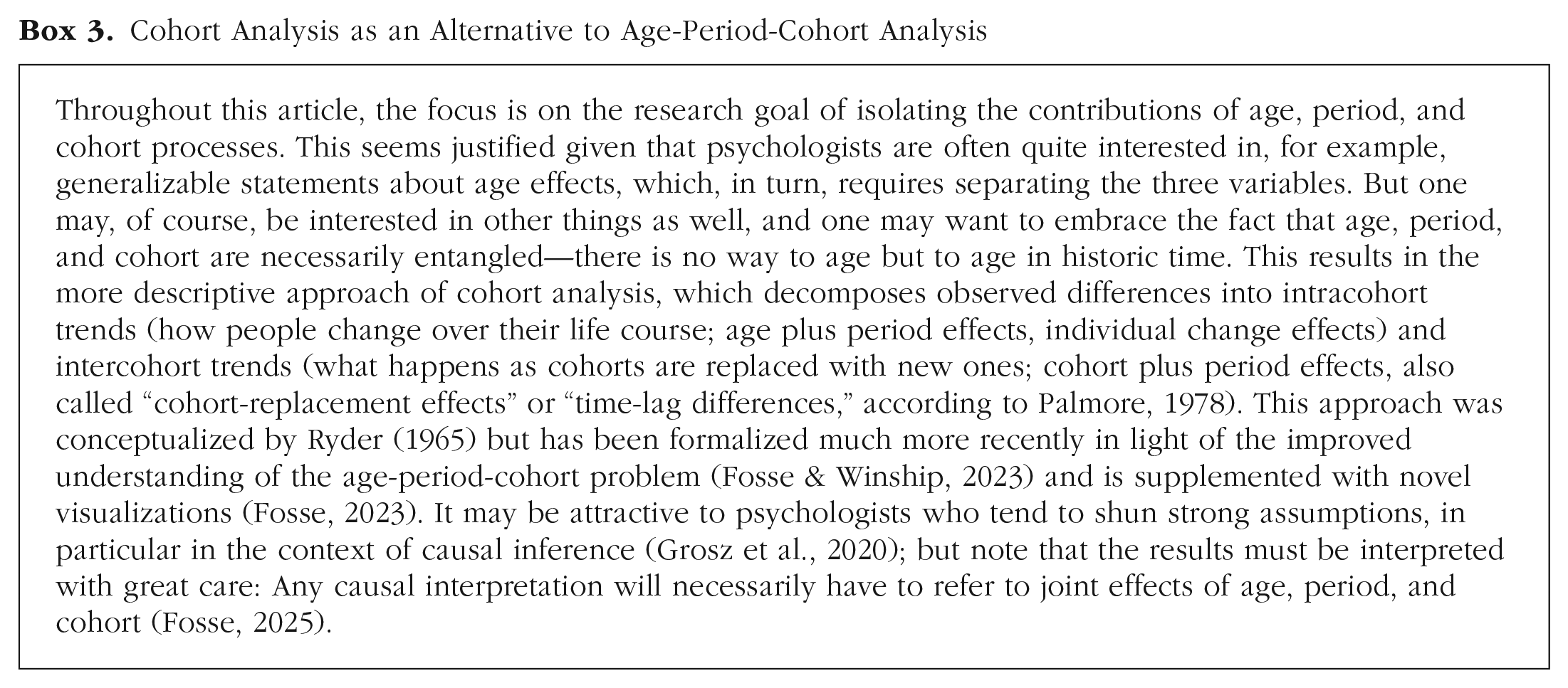
One way forward is to abort the whole mission. Given the strange counterfactuals involved in the effects of interest (Box 1), one may decide that age-period-cohort analyses are not particularly fruitful and turn to something else, such as investigating causes that may more directly affect the outcome of interest—including those that may ultimately mediate the effects of temporal variables. 3 Alternatively, one may choose the more descriptive approach of cohort analysis (Box 3), which incorporates an up-to-date understanding of the problem but does not aim to disentangle the underlying effects.
Cohort Analysis as an Alternative to Age-Period-Cohort Analysis
But what if one still does want to make statements about age effects, period effects, or cohort effects? In that case, one will need a way to pick a plausible combination of effects from the infinitude of combinations that are equally compatible with the data. This will necessarily involve (fallible) assumptions about either the involved mechanisms or the effects of interest themselves.
Assumptions about mechanisms
The mechanism-based approach developed by Winship and Harding (2008) starts from the observation that age, period, and cohort are just stand-ins for associated processes. The core idea is that if one knows (and measures) all mechanisms through which one of the three temporal variables operates (e.g., all mediators of the effects of period on the outcome), one can, in turn, determine the effects of that variable (e.g., the period effects). 4 At that point, the age-period-cohort problem has been solved because determining the effects of one of the variables determines which of the possible solutions to the identification problem to settle on. Estimation can be carried out with structural equation models (containing age, period, and cohort and the assumed mediators), which even allows one to assess model fit and thus reject empirically implausible models. The major downside of this approach is the very strong assumption that one can fully explain how age, period, or cohort affect the outcome and that all mediators were appropriately measured. Bijlsma et al. (2017) provided an extension of this approach, highlighted pitfalls, and suggested best practices.
Assumptions about the effects of interest
Assuming some effects are zero
More commonly used approaches instead rely on assumptions about the effects of interest themselves, although the degree of transparency with which they do so varies considerably. Maybe the simplest type of assumption one can make is that one of the variables does not have any effect on the outcome. At that point, one has settled on the effects of one variable (they are zero, by assumption) and again solved the age-period-cohort problem as a whole. For example, above, I mentioned longitudinal studies on personality development in which the within-individuals change over time is interpreted as age effect; this interpretation would be warranted under the assumption of no period effects, which, of course, should be spelled out transparently (for one attempt to do so, see Seifert et al., 2024). If one is willing to assume that age, period, and cohort do not interact, then, as outlined above, the nonlinearities can be identified based on the data alone—thus, under the assumption of no interaction, one needs to assume only that there is no linear period effect (i.e., no overall time trend that affects everybody’s personality in the same way). But researchers can also pick a different way forward that allows for interactions if they assume that period has no effects whatsoever—in that scenario, they can simply look at the age trajectory for each cohort and interpret it as the corresponding cohort-specific age effects.
The assumption that some of the effects are zero can be “implemented” in standard statistical models by simply omitting variables. The details of these models will depend on which effects are of interest and what data are available. Kratz and Brüderl’s (2021) analysis of the age trajectory of happiness provides an excellent illustration of how the choice of the precise statistical model can be justified rigorously.
Constraints imposed by statistical models
As already discussed, another way to pick a solution is with the help of more or less out-of-the-box statistical models, such as the hierarchical age-period-cohort model (discussed in Box 2) or the intrinsic estimator. As discussed above, the big weakness of these approaches is that they solve the identification problem through obscure constraints that depend on features that have nothing to do with the underlying effects of interest, such as the design with which the data were collected. That said, their big advantage is that they can be easily realized because software implementations are often readily available.
If the constraints imposed by the models happen to map onto the assumptions one is willing to make, results may turn out sensible—for example, if one is willing to assume that there is no linear cohort trend, the standard hierarchical age-period-cohort model applied to data in which cohort has the broadest range of the three temporal variables may be a fruitful way forward. But if this way forward is chosen, transparency about the underlying assumptions becomes even more crucial because otherwise, readers may miss that assumptions are involved in the first place.
Bounding analysis
In contrast, the bounding-analysis approach developed by Fosse and Winship (2019b) very deliberately focuses on explicit assumptions. The central idea is that one starts from the canonical solution line (e.g., Fig. 1) and narrows it down to a range of values that are plausible given one’s assumptions about what the age, period, and cohort effects should look like. For example, one may discard parts of the line because they imply implausibly large effects. Although a combination of very large age, period, and cohort effects that cancel each other out may be compatible with data in which there are only small group differences, such an explanation would not be particularly parsimonious. One may also add assumptions about the directionality of linear effects, such as “overall, health complaints go up with age,” discarding all parts of the line that imply a negative linear age effect. And one can add even more specific assumptions about certain stretches of the overall trajectories. For example, one may assume that health complaints monotonically increase between ages 50 and 70. This can further constrain the linear effects because the overall effects are the sum of the linear effects and the nonlinearities. For example, if the age nonlinearities on their own imply a decrease in health complaints from age 50 to age 51, they need to be offset by a positive linear age effect of sufficient strength to generate the assumed monotonous increase. Other types of assumptions are also imaginable—one could, for example, assume that the effects of one temporal variable do not exceed the effects of another one or that the cohort effects are related to the period effects in such a manner that cohorts are shaped by the period effects they experience as they grow up.
Once one has incorporated all of one’s assumptions, the canonical solution line will be restricted to a more or less narrow range of plausible solutions, and one can plot the various trajectories of age, period, and cohort effects that are implied by the remaining solutions to put bounds on the effects of interest. The bounding-analysis approach is a great way to better understand what is going on in the data and develop some understanding of how the conclusions about the various effects are interrelated. It thus provides educational value even if one may eventually settle on a different statistical model. Thus, I provide a small empirical illustration; the corresponding code can be found on OSF (https://osf.io/rzc4u/).
Empirical Illustration: Bounding Analysis of German Attitudes Toward Working Mothers
Data and measures
The German General Social Survey (Allgemeine Bevölkerungsumfrage der Sozialwissenschaften [ALLBUS]) is a project of GESIS (Leibniz Institute for the Social Sciences) and has collected a wide selection of variables from people in Germany every other year since 1980 (with minor deviations in schedule because of the German reunification). It is not a longitudinal study, so different people are sampled every wave. After a brief registration, the data can be downloaded for free. Here, I analyze the cumulated data, Version 1.1.0 (GESIS-Leibniz-Institut für Sozialwissenschaften, 2024).
I am interested in three items assessing respondents’ attitudes toward working mothers: “A working mother can have a relationship with her children that is just as loving and trusting as a non-working mother,” “A small child will surely suffer when their mother works,” and “It is even good for a child if the mother works and is not only focused on the household.” These were answered on a 4-point response scale (1 = fully agree, 4 = do not agree at all), and all items are recoded so that higher values indicate agreement with the notion that it is good (or at least not actively bad) for children if their mother works (“approval of mothers working”). All items are moderately correlated (.39 < r < .49), resulting in an aggregate scale with Cronbach’s α = .69. The items were included in the survey years 1982 and 1991 and then starting from 1992, in every other survey (i.e., every 4 years) until 2016. Because the model I am going to fit requires that all temporal variables (age, period, cohort) have equal-width coding, I limit myself to the data from 1992 to 2016 waves and recode age and cohort to bins that match the period variable (3 years per bin, so that every fourth year starts a new bin). 5 In my analysis, I will put aside a lot of concerns that one would have to consider if the main purpose of this article was to provide an empirical answer, such as the sampling scheme of ALLBUS and a change in the assessment mode in 2000.
I include only people who answered the items, reported their age, and are younger than 70 years old (to ameliorate concerns about selective mortality at higher ages). The resulting sample includes 17,047 people with an average age of 43.83 years (SD = 14.19). Data were collected in 1992, 1996, 2000, 2004, 2008, 2012, and 2016, and the range of included cohorts is very wide, as one would expect given the study design (respondents born between 1923 and 1998). I used the R package apcR that Fosse and Winship provided on their website (https://scholar.harvard.edu/apc/software-0; downloaded version April 2024).
Identification assumptions
To conduct my bounding analysis, I need to make assumptions about the effects of age, period, and cohort on people’s attitudes toward working mothers. Here, I am going to work with the following assumptions:
The linear period effect should be positive: Across the observed periods (1992–2016), there is an overall trend that approval of mothers working increases, driven by period processes.
The linear cohort effect should be positive: Across the observed birth cohorts (1923–1998), there is an overall trend that approval of mothers working increases, driven by cohort processes.
Among the youngest cohorts in the data (1983–1998), there is a monotonous increase in approval, driven by cohort processes.
The first two assumptions follow from the idea that times have been changing: It has become a lot more normative for mothers to work. Because these historic changes in norms should affect people of all ages (to at least some extent), approval should go up. Likewise, younger cohorts grew up under norms increasingly in favor of working mothers (or at least less opposed to them), so approval should go up with them as well.
On top of these two fairly straightforward assumptions about linear effects, I also explore the implications of a third, more restrictive assumption that invokes monotonicity regarding the overall cohort effects. Although the main purpose of this assumption in the context of this article is to illustrate the mechanics of cohort analysis, it is still motivated by a priori considerations. Specifically, children who grow up in periods in which more of their peers’ mothers are working should be less likely to think that working mothers are bad for children. So if one identifies a period in which maternal employment rose, one would expect a corresponding positive cohort effect for the cohorts that were children in those times. Because of German history, maternal employment rates in Germany do not follow a simple pattern 6 ; however, from 2005 to 2014, maternal employment seems to have increased across the board, considering both East Germany and West Germany and both full-time and part-time employment (Barth et al., 2020). Assuming that this affected the opinions of individuals who grew up in those times, I expect a monotonic increase in approval from the 1983–1986 cohort (who had already come of age in 2005) to the youngest cohorts in our data (1995–1998).
Analyses and results
First of all, to get a feeling for the trends in the data, one can look at the average approval. Figure 6 illustrates four possible ways to plot these means, depending on which temporal variable is chosen for the horizontal axis and which temporal variable is used to connect the dots. 7 As explained above, even if those graphs look suggestive, they cannot reveal the age, period, and cohort effects. However, they do reveal combined effects. For example, for each single cohort, as time passes, approval goes up quite clearly. This already tells one that the linear age effect and the linear period effect must add up to a positive number.

Different ways to plot the average approval of mothers working, measured in the German General Social Survey, across age, period, and cohort. Approval can range from 1 to 4 (overall SD = 0.75 scale points).
To get a more systematic understanding of which combinations of effects are compatible with the data, I used the function runapc() to estimate the linearized age-period-cohort model. In essence, this is a linear model including the linear effects of age and cohort (but not period) and all categorical effects of age, period, and cohort. Note that the model has been parametrized so that the nonlinearities (to which the age-period-cohort problem does not apply, assuming no interactions) are separated from the linearities (to which it does apply).
The output includes a coefficient for the linear age effect, which should be interpreted as the sum of the linear age effect and the linear period effect (a quantity called “
Canonical solution line and nonlinearities
The analysis results, which one can directly derive from the linearized age-period-cohort model, are the canonical solution line depicting the possible combinations of linear effects underlying my data (Fig. 7a) and the nonlinearities (Figs. 7b–7d). The location of the canonical solution line (Fig. 7a) already informs one that the data are not compatible with a data-generating mechanism in which, for example, both the linear period effect and the linear cohort effect are negative: The line simply does not pass through that part of the graph.

Canonical solution line and nonlinearities of the age-period-cohort analysis of approval of mothers working. Nonlinearities lines provide locally smoothed estimates (locally estimated scatterplot smoothing, ggplot2 default parameters), weighting the nonlinearities by the underlying sample sizes.
Because I already assumed that both the linear period effect and the linear cohort effect are positive, I can discard further parts of the canonical solution line and narrow it down even more (grayed out in Fig. 7a). However, at this point, one cannot yet deduce whether the linear age effect is positive or negative; the undiscarded parts of the line are compatible with a linear increase of up to +0.77 scale points per 40 years (corresponding to +1.03 SD per 40 years, or +0.26 SD per decade) or a linear decrease of up to −0.15 scale points per 40 years (−0.20 SD per 40 years, or −0.05 SD per decade).
My third assumption—a monotonous increase among the youngest cohorts—can potentially narrow the range of possible solutions even further. The cohort nonlinearities (Fig. 7d) imply a decrease among the youngest cohorts when considered in isolation. Thus, to arrive at the assumed overall monotonous increase, the nonlinearities need to be “compensated for” by a positive linear cohort effect of sufficient strength. To determine how strong that linear effect needs to be, I first have to settle on how strong the nonlinear increase is. As it turns out, because of the survey design, there are fairly few respondents who belong to the youngest cohorts (1983–1986: n = 520; 1987–1990: n = 370; 1991–1994: n = 187; 1995–1998: n = 69). Thus, to ensure that I do not overestimate the decrease implied by the nonlinearity, I instead relied on the depicted smoothed estimates (LOESS with the ggplot2 default parameters) for which the nonlinearities are weighted by the sample sizes underlying their estimation. I determined the strongest decrease implied by these smoothed nonlinearities (which turns out to be approximately −0.003 scale points per year) and calculated the necessary positive linear effect (per 40 years) to cancel it out and ensure a monotonous increase, (−1) × (−0.003 scale points per year) = +0.12 scale points per 40 years. Thus, the third assumption further narrows the stretch of the canonical solution line that I can consider plausible, but only barely so (Fig. 7e). 8
Plotting the resulting bounds
Three assumptions have thus narrowed the range of plausible linear effects. To spell out these ranges, the linear age effect should be between −0.025 and 0.77 scale points per 40 years, the linear period effect should be between 0.01 to 0.8 scale points per 40 years, and the linear cohort effect should be between 0.12 and 0.92 scale points per 40 years. The endpoints of these ranges mark the most “extreme” solutions to the age-period-cohort problem compatible with the data, marked in red and blue in Figure 7e.
To understand what these numbers mean, one can put them back together with the nonlinearities and plot the resulting implied effect trajectories. This finally results in the bounds, depicted in Figure 8a.

Bounds on the age, period, and cohort effects on approval of mothers working resulting from my analysis. (a) The point estimates of the most extreme solutions and the trajectory in the middle between the two extremes. (b) The confidence intervals for both the middle and the extreme trajectories. Approval can range from 1 to 4 (overall SD = 0.75 scale points).
Figure 8 shows the implied trajectories for three different points on the canonical solution line. Two of them (red solid line and blue dashed line in Fig. 8a) result if one picks one of the most extreme solutions on the remaining stretch on the line (marked in Fig. 7e). The middle trajectory represents the “middle” solution, which corresponds to the midpoint of the remaining stretch of the canonical solution line.
What do these bounds tell one about how age, period, and cohort affect people’s approval of mothers working in my data? Considering age, one cannot rule out that the trajectory is quite flat (minimum linear age effect), with a slight decrease starting at approximately age 42. However, the data are also compatible with rather pronounced increases over the life course. Taken together, one can at least rule out that there is a strong decrease with increasing age. Considering period, again, one cannot rule out that the trajectory is quite flat (minimum linear period effect) or somewhat steeper (maximum linear period effect) over the years observed. Even in the steepest case, approval actually goes slightly down from 2012 to 2016—so based on my assumptions, it does not look like any trend of increasing approval extends to the latest wave of data. Finally, the cohort trajectory is the one that looks most dramatic, but one should keep in mind that the cohort variable also spans the largest number of years. Here, based on my assumptions, it clearly follows that from the oldest cohort up until the circa 1964 cohorts, approval of mothers working increased quite a bit. But the bounds show that it is quite uncertain what happens after that—approval may further increase in an almost linear fashion because of cohort processes, but it may also stagnate.
Although I looked at the trajectories independently, choosing a point on the canonical solution line immediately determines all three trajectories at once. So, for example, if one picks the solution that implies that there is very little happening with age (solid red line on the left in Fig. 8), one would also have to conclude a more pronounced period increase (solid red line in the middle in Fig. 8) and a cohort increase among the oldest cohorts that eventually levels off (solid red line on the right in Fig. 8). Put another way, there may be trajectories of age, period, and cohort effects that lie within the respective bounds when considered in isolation but that cannot simultaneously be true.
Incorporating sampling variability
Up to this point, the bounds take into account uncertainty because of the age-period-cohort problem but not additional uncertainty resulting from statistical estimation. To be able to generate, for example, confidence intervals (CIs), one can bootstrap the whole bounding procedure—that is, one can resample my data repeatedly and implement the whole estimation procedure, 9 which results in a distribution of bounds that one can use to draw further inferences. This is currently not implemented in the apcR package, so I have to rely on a custom bootstrap setup that can be found on OSF (here implemented in the boot package; Canty & Ripley, 2022; Davison & Hinkley, 1997). Figure 8b shows the resulting percentile bootstrap CIs for the bounds and the solution in the middle between the bounds. One can further use the bootstrapped results to test specific hypotheses. For example, is the period decrease in approval from 2012 to 2016 statistically significant? It turns out that this is the case for the lower bound (decline of −0.12 scale points, 95% CI = [−0.17, −0.07]) and the middle solution (decline of −0.08 scale points, 95% CI = [−0.13, −0.03]) but not for the upper bound (decline of −0.04 scale points, 95% CI = [−0.09, 0.01]). Thus, whether one concludes only stagnation or even a decrease in approval between the last two included survey years remains open unless one narrows the bounds further with the help of additional assumptions.
Note that if one was analyzing longitudinal data, during the resampling stage of the bootstrapping procedure, one would randomly draw whole individuals (including all of their observations) rather than just individual observations to ensure that the calculated CIs correctly take into account dependencies in the data. Furthermore, instead of bootstrapping, one could rely on a Bayesian approach to incorporate uncertainty; after all, the assumptions that one uses to narrow down the space of possible solutions are prior beliefs. Fosse (2021) developed such an approach.
Discussion
The age-period-cohort identification problem is a fundamental problem that researchers encounter every time they want to make statements about how age, period, or cohort affect any outcome. It requires that researchers make informed decisions and take a stance on which assumptions they are willing to make (or not) to identify the effects of interest. These assumptions determine whether empirical answers are possible in the first place—for example, if one operates under the assumption that everything plausibly interacts and that effects may take on any conceivable shape, then it follows that no statements about age, period, or cohort effects are possible. If, instead, one is willing to make stronger assumptions, one may arrive at point estimates or at least bounds within which the true estimates lie, always conditional on the validity of one’s assumptions.
Looking back, the psychological literature is filled with claims about age effects and to a lesser extent, claims about cohort effects and the occasional period effect. These claims have to rest on assumptions, but given the limited awareness of the full scope of the age-period-cohort problem, these are usually not spelled out. A central task when trying to make sense of the published literature is thus first, figuring out which assumptions are necessary to arrive at the authors’ conclusion and second, determining whether these assumptions are plausible. In this article, I have hopefully provided a toolkit for the first step. The second step will rely on the readers’ domain expertise and their often subjective assessment.
Moving forward, the onus of spelling out assumptions should, of course, be on the authors who make claims about age, period, and cohort effects. These assumptions exist regardless of the statistical approach chosen and should be spelled out in a manner that they can be understood by an informed reader. Reviewers and editors can help with this shift by asking a simple question: “Due to the age-period-cohort identification problem, all claims about age/period/cohort effects rely on identification assumptions. Which assumptions are necessary to arrive at your conclusions? Why do you consider them defensible?”
It is an open question how well the field of psychology can defend the assumptions necessary to make any claims about the effects of interest. For example, if one wanted to conduct an age-period-cohort analysis of personality, one might draw on personality maturation to identify the effects of interest (“conscientiousness goes up with age”), but one’s understanding of personality maturation itself rests on empirical findings that may be wrong because of the age-period-cohort problem. Researchers thus have to draw on other knowledge about the world: Does anything happen between these ages that makes one think the outcome should go up or down, on average? Does one know of any historic events that should lead to certain period patterns? Does one know of anything that may have affected people of a certain age at a specific point in time, resulting in to-be-expected cohort effects?
How well researchers can answer these questions will vary between different outcomes and strongly depend on domain expertise. For example, for outcomes related to public opinion, researchers may be able to make plausible assumptions about period effects; for outcomes more closely related to biological processes, researchers may be able to make plausible assumptions about age effects. For many psychological constructs, it may be genuinely hard to come up with plausible assumptions for any type of effect given limited knowledge and additional measurement issues. Ideally, moving forward, researchers can establish a culture in which assumptions are communicated transparently and subjected to critical debate, allowing the field to systematically accumulate reliable knowledge about how age, period, and cohort affect people’s mind and behavior.
Footnotes
Acknowledgements
Malin Benjes and Stefan Schmukle repeatedly provided helpful comments on drafts of this article. Furthermore, Frederik Aust, Malcolm Barrett, Andrew Bell, Malin Benjes, Saloni Dattani, Ethan Fosse, Isabella Ghement, Benjamin Hankin, Kevin King, Brent Roberts, Lena Roemer, and Christopher Winship provided helpful comments on the initial draft. Malcolm Barrett also provided a code review of an earlier version of the analysis scripts. The Allgemeine Bevölkerungsumfrage der Sozialwissenschaften data used in this article are made available to the scientific community by GESIS (Leibniz Institute for the Social Sciences). This publication was supported by the Open Access Publishing Fund of Leipzig University.
Transparency
Action Editor: Rogier Kievit
Editor: David A. Sbarra
Author Contributions