Sage Journals: Discover world-class research

Abstract

Before conducting statistical analyses, scholars and researchers often have specific hypotheses about differences between groups of means. Their hypotheses are frequently tested by applying post hoc comparisons with statistically significant simple or interaction effects. With the exception of exploratory studies, using post hoc comparisons can increase Type I error rates and decrease statistical power. A well-known solution involves planning comparisons before the study. However, the coding of such planned comparisons can be difficult to understand and implement, especially for customized comparisons and interaction effects. In this tutorial, we aim to reduce such difficulties by examining all the possible types of planned comparisons, even the customized ones, for both main and interaction effects. In this tutorial, a Shiny App coded in R and called “appRiori” is presented. appRiori is coded to help in understanding both the logic behind the planned comparisons and the way to interpret them when a model is tested. By using empirical examples on reproducible data, we explain how to code any default planned comparison executable in R. Moreover, through some features of appRiori, the customization of planned comparisons is shown, even on interaction effects, such as the possibility of creating customized contrast through click-and-drop menus. For each step, the R code related to the planned comparison is provided. Implications and fields of use of planned comparisons and appRiori are discussed.

Keywords

contrasts planned comparisons Shiny App open data

Although scientific progress requires increasingly complex data analyses, most of the time, researchers need to understand how to compare means (sometimes trends) between groups. Statistical comparison of such means can be straightforward, especially in models testing the relationship between a single numeric response variable and a single categorical predictor with two levels (e.g., analysis of variance [ANOVA] and linear or nonparametric models). The situation becomes more difficult when the single predictor has more than two levels or when researchers are also interested in testing interaction effects. These situations are usually approached in two ways. In one strategy, a model is tested, and overall statistics such as $F$ or $χ^{2}$ are extracted for both simple and interaction effects. Whenever a statistically significant effect (Cohen, 1994; i.e., $p < . 05$ ) is found, a series of post hoc analyses (usually t tests or z tests) is performed to identify which pairs of conditions are statistically different. This strategy is useful when the study is exploratory, that is, when there is no previous knowledge about the potential effects. However, this strategy has several disadvantages. An omnibus statistic suggests only that there is a difference between some means but does not provide any information about specific differences. Moreover, running multiple post hoc comparisons among all possible differences reduces statistical power. It is not rare that comparisons that are not of interest can make those of interest nonsignificant (Thompson, 1990). In fact, especially when there is some knowledge about the differences among conditions or the researchers have some hypotheses about them, all the comparisons that do not investigate such differences subtract power (and often the aimed statistical significance) from the target ones. The more the number of tested comparisons increases, the higher the Type I error increases, necessitating an adjustment of the p values (e.g., Bonferroni or false-discovery-rate methods; Westfall & Young, 1993). Finally, having a priori hypotheses is considered a fundamental best practice in several branches of science (e.g., psychology or social sciences), especially in recent years, because preregistrations have become a widespread practice.

If researchers have specific hypotheses, guided by either ideas or previous knowledge on the topic, another strategy is to set specific planned comparisons or contrasts among the observed conditions’ means. These comparisons offer three advantages. First, a priori contrasts allow for balancing the trade-off between Type I and Type II errors (Garofalo et al., 2022). In particular, minimizing the number of multiple comparisons reduces the chance of observing an effect that does not actually occur; consequently, statistical power increases (Davis, 2010). This applies to both simple and interaction effects (Graham, 2000; Seaman et al., 1991). A second related advantage is that some a priori comparisons could emerge as statistically significant compared with the same (nonsignificant) post hoc comparisons (Kwon, 1996). Finally, this type of comparison allows the researcher to be more thoughtful in designing the experiment and the analyses, thereby increasing the quality of the work (Buckless & Ravenscroft, 1990; Kuehne, 1993; Kwon, 1996; Ruxton & Beauchamp, 2008).

Although the consensus on the advantages of a priori contrasts over post hoc comparisons has been consolidated (Kuehne, 1993; Thompson, 1990) and some interesting works provide suggestions and guide on contrast analysis (Haans, 2019; Rosnow et al., 2000), post hoc comparisons are still preferred. Ruxton and Beauchamp (2008) pointed out that only a very small percentage of studies used a priori contrasts, even when researchers clearly stated specific hypotheses at the beginning of the article. This evidence has been found independently in various research areas. A study by Garofalo and colleagues (2022) examined several articles in the neuroscience literature and found that in cases of interaction effects, 98% of articles used post hoc comparisons, and only the remaining 2% used planned comparisons. Likewise, Brehm and Alday (2022) conducted a metascientific study examining more than 3,000 articles in psycholinguistics. The authors found that fewer than one third of the studies explicitly stated which planned comparisons were used. This lack of use persists and is related to issues of reproducibility (Brehm & Alday, 2022) and sometimes the rejection of articles (Agathokleous & Yu, 2022).

A possible explanation for such limited use could be that a priori contrasts can be difficult and complicated (Agathokleous & Yu, 2022) in terms of (a) understanding the logic and formal aspects; (b) application, that is, how to code them with statistical software; and (c) interpretation of their statistical effect without using an overall statistic. These issues are more evident not only for well-known contrasts, such as treatment, sum, or Helmert, but also when researchers need to set customized contrasts even without considering interaction effects. Indeed, the difficulty in programming customized contrasts is one of the main reasons behind the limited use of this type of comparison. The same applies to the use of planned comparisons in the case of interaction effects. Manuals and articles addressing interaction effects often use technical, ambiguous, or cumbersome terms, making such constructs accessible only to researchers with a strong formal background. Some statistical software provides dedicated commands or shortcuts to insert the comparisons to be tested in a potential model: Nonetheless, it is often unexplained how such comparisons are then tested inside the model and how the model coefficients (e.g., in case of regression) are calculated. As a result, some readers continue to have difficulty understanding planned comparisons for models for which software shortcuts are not available, so they do not use them (Garofalo et al., 2022).

There is a consensus on the need for tools to help researchers with planned comparisons in a way that does not rely solely on default settings in statistical software, which can be misunderstood (Brehm & Alday, 2022), but, rather, in an easy and intelligible way. Nonetheless, such need has received poor or no response. The difficulty in applying planned comparisons can be summarized in four issues: (a) understanding and learning the logic behind a priori contrasts, (b) directly planning both well-known and customized contrasts, (c) setting contrasts not only for simple effects but also for interactions (e.g., two-way and three-way), and (d) coding the corresponding ready-to-use code of the statistical software in a way that such code can be applied directly before running the analysis.

In the present article, we aim to address each of these critical issues by providing a tutorial on (a) how planned contrasts work, (b) which kinds of contrasts can be used, (c) how to set customized contrasts, and (d) how to obtain the R code for such contrasts (R Core Team, 2021) for both simple and interaction effects. A Shiny App coded in R (Chang et al., 2021), called “appRiori,” has been programmed to make each step understandable and reproducible.

The article is organized as follows. In the next section, a brief formal explanation of what contrasts are and their role in handling categorical variables in linear models is provided. In the “Type of Contrasts” section, an overview of all types of contrasts is provided, with a focus on the customized and interaction ones. In addition, a brief overview of the Shiny App is given. In the “Empirical Examples” section, three examples of how to select, plan, use, and interpret specific contrasts are provided, even with data available in R. Finally, the implications of using both planned comparisons and the proposed app are discussed.

How to Get Away With Planned Comparisons: A Guide

(Brief) Theoretical background

In the present subsection, we aim to provide a brief overview of the flow that starts from hypothesis definition to the estimation of the linear model’s coefficients related to the target comparisons. Mathematical and more in-depth descriptions of matrix algebra and linear models (Howell, 2010; Schad et al., 2020) are beyond the scope of this article. Hypotheses regarding differences between means or combinations of means are tested with contrasts. Contrasts are weighted linear functions (usually of means; Baguley, 2012) that encode and quantify the performance or comparisons among a set of means. In other words, contrasts make it possible to collapse several comparisons among the levels of a categorical variable into a unique function, as if they were a single effect. Contrasts are estimated within linear models, such as regression, generalized, and mixed models. In the following paragraphs, the path from the research questions to the contrasts’ estimations is provided.

Example 1

Consider a simple experimental question: Do researchers using planned comparisons feel happier than researchers who do not use them?

To answer this question, it is possible to create a fictional dependent variable Y, ranging from 1 (lowest level of happiness) to 10 (highest level of happiness). Assume now to recruit 10 researchers and assign them to two groups, paired in every aspect except for the frequency of use of planed comparisons: The former group regularly uses planned comparisons, and the latter does not use them at all. In this way, the independent variable of the experiment is a categorical variable $G$ , having only two levels (Group $g 1$ vs. Group $g 2$ ), with means $μ_{1}$ and $μ_{2}$ , respectively. For a long-format database of this example, see Table 1.

Table 1.

Example of Database

Subject ID	Happiness	G
1	8	g1
2	7	g1
3	9	g1
4	6	g1
5	5	g1
6	8	g2
7	7	g2
8	4	g2
9	4	g2
10	3	g2

In this case, it is clear that the contrast is comparing the means in the dependent variable of the two groups. In terms of hypotheses, we are testing the null hypothesis $H_{0} : μ_{1} - μ_{2} = (1) μ_{1} + (- 1) μ_{2} = 0$ . To test this hypothesis in a linear model, which works with numbers and not with labels, assign the value 1 to the cases in Group $g 1$ and the value −1 to the cases in Group $g 2$ . These values can be called contrasts weights because they contribute to estimating (i.e., weight) the parameters of the (future) statistical model (Schad et al., 2020). The preliminary hypotheses and their related contrast weights can be practically arranged into a matrix called the “hypotheses matrix,” where rows represent the hypothesis to test and columns represent the weight to assign to a group (or level). The hypothesis matrix in this example is the following:

H = [\begin{matrix} 1 & - 1 \end{matrix}],

(1)

or, coherently with the position of the levels in a database, in its transposed version $H^{T}$ :

H^{T} = [\begin{matrix} 1 \\ - 1 \end{matrix}] .

(2)

Representing hypotheses using matrices has several advantages: From a conceptual point of view, $H$ makes it clear that in the case at hand, the contrast compares the means of two groups by computing the difference between the Group $g 1$ mean and the Group $g 2$ mean; moreover, it gives the chance of collecting all the hypotheses into a single mathematical object that, in turn, can be used to estimate desired comparisons via a linear model. Crucially, collecting all the hypotheses in a matrix makes clear how different hypotheses influence each other when estimated in a model (see following sections). To understand how this hypotheses matrix can be applied to data to test mean differences via a linear model, it is necessary to take into account the formula of the linear model in matrix notation:

Y = X β + ϵ,

(3)

where $Y$ is a $n \times 1$ matrix of observed responses, $X$ is a $n \times k$ “design matrix” of $k$ independent variables and $n$ observations, $β$ is a $k \times k$ matrix of unknown parameters that we want to estimate, and $ϵ$ is a stochastic error component. It is well known that by applying the ordinary least squares criterion to Equation 3, it is possible to estimate the matrix of $\hat{β}$ parameters through the following formula:

\hat{β} = {(X^{T} X)}^{- 1} X^{T} Y .

(4)

From Equation 4, it can be observed how a set of operations are performed on matrix $X$ (i.e., ${(X^{T} X)}^{- 1} X^{T}$ ) before multiplying it to the observed responses ( $Y$ ). This set of operations is known as “generalized matrix inverse,” and it allows to convert the matrix $X$ into a set of weights that can be combined to observed data (i.e., matrix $Y$ ) to obtain estimated regression coefficients (Schad et al., 2020). When the generalized matrix inverse is applied to the hypothesis matrix $H$ , it is possible to obtain the contrast matrix $C$ ,

C = [\begin{matrix} 0.5 \\ - 0.5 \end{matrix}],

(5)

where, in the case at hand, the weights in matrix $C$ are the ones that can be later assigned to the variable $G$ to estimate regression coefficients. By definition, a contrast matrix $C$ contains the groups or levels of a variable in the rows, and the specific comparisons to be tested are in the columns, along with their corresponding weights. In other words, the contrast matrix $C$ can be conceived as a way to adapt theoretical hypotheses (i.e., $H$ ) into a form that is usable in the context of the linear model, enabling the formulation and testing of hypotheses about the relationships between the independent variables and the dependent variable.¹

Statistical software has different ways to go back and forth between hypotheses, contrasts matrices, and regression coefficients. In the present tutorial, the statistical software R is used (R Core Team, 2021). For a detailed introduction to R, see R Core Team (2024). The code to define both hypothesis and contrast matrices of Example 1, such as their implementation to obtain regression coefficient starting from data of Table 1, is shown in Listing 1.

Listing 1: R code for hypothesis and contrast matrices to estimate regression coefficients starting from data of Table 1

It can be observed how in R, the generalized matrix inverse of the hypothesis matrix $H$ can be obtained by applying a specific function named ginv(), which can be found in the MASS package (Venables & Ripley, 2002). Once the contrasts matrix $C$ is defined, it can be assigned to the variable G trough the contrasts() function. In this way, the contrasts weights will be assigned to each condition in the database, ready to be passed to the regression model via the lm() function.

Once the coefficients are estimated, it is possible to note that the slope of the model is equal to $b = 1.8$ , which is exactly the difference between the mean of Group $g 1$ and the mean of Group $g 2$ . In fact, by multiplying each group mean (i.e., $μ_{g 1} = 7$ , $μ_{g 2} = 5.2$ ) by the contrast weight initially formulated in the hypothesis matrix $H$ (i.e., 1 and −1) and subtracting these products, the slope coefficient can be obtained, that is, $(1 \times 7) + (- 1 \times 5.2) = 1.8$ . Consequently, it is possible to answer the research question by implementing the formulated hypotheses.

The importance of the contrast matrix

The previous subsection provided the general procedure for performing contrast analysis with a linear model, testing the exact hypothesis one has in mind. In particular, the hypotheses are defined in the $H$ matrix as described above, the corresponding $C$ matrix is obtained by applying the generalized matrix inverse function to $H$ , and the weights obtained in $C$ are used to code the categorical variable into the linear model. The contrast matrix $C$ has a central role in the estimation of the results of a linear model. As suggested by Schad and colleagues (2020), a contrast matrix, via the generalized matrix inverse function, represents a hub between (a) the way of defining a set of hypotheses that researchers have on certain independent variables and (b) the way of defining weights that will be combined with data to estimate regression coefficients. This connection can be particularly useful in comparisons involving more than two groups.

Example 2

We now expand the data of Example 1. Assume you add a new group to the former two (i.e., researchers who frequently use planned comparisons and who use only post hoc comparisons) by recruiting 10 further researchers who do not use comparisons at all.

At this point, the categorical variable $G$ has three levels ( $g 1$ , $g 2$ , $g 3$ ) with means $μ_{1}$ , $μ_{2}$ , and $μ_{3}$ , respectively. Assume that the aim is now changed: testing the difference between subsequent levels, that is, $g 2$ versus $g 1$ and $g 3$ versus $g 2$ . This kind of comparison is frequently used in research and tested through the so-called repeated contrasts (or sliding difference contrasts). Equation 6 shows the hypothesis matrix and its transposed version (for more details on this type of contrast, see “Types of Contrasts” section):

H = [\begin{matrix} - 1 & 1 & 0 \\ 0 & - 1 & 1 \end{matrix}] H^{T} = [\begin{matrix} - 1 & 0 \\ 1 & - 1 \\ 0 & 1 \end{matrix}] .

(6)

It can be observed that the first column refers to the first hypothesis: The condition $g 1$ is coded with the value $- 1$ , and the condition $g 2$ is coded with the value $1$ . The last level is not included in such comparison, so it is coded with the value $0$ . Likewise, the second column refers to the second hypothesis: The condition $g 2$ is coded with the value $- 1$ , and the condition $g 3$ is coded with the value $1$ . The first level is not included in such comparison, so it is coded with the value $0$ . In fact, in terms of null hypothesis testing, the null hypotheses would be the following:

H_{0_{c o m p a r i s o n 1}} : μ_{2} - μ_{1} = (- 1) \times μ_{1} + (1) \times μ_{2} = 0

H_{0_{c o m p a r i s o n 2}} : μ_{3} - μ_{2} = (- 1) \times μ_{2} + (1) \times μ_{3} = 0 .

By applying the generalized matrix inverse to the previous hypothesis matrix $H$ , the following contrast matrix $C$ can be obtained:

C = [\begin{array}{r} - 0.67 & - 0.33 \\ 0.33 & - 0.33 \\ 0.33 & 0.67 \end{array}] .

(7)

The reading of the comparisons in matrix $C$ may be less straightforward than the same ones in matrix $H$ . Therefore, it is useful to use $H$ to understand the stating hypotheses and use $C$ to implement them into a potential statistical model. The following code shows the use of repeated contrast in Example 2.²

Listing 2: R code for hypothesis and contrast matrices to estimate regression coefficients in case of repeated contrasts

Even in this case, it can be checked that the first slope of the model is equal to $b = - 1.8$ , that is, exactly the difference between the mean of group $g 1$ and the mean of group $g 2$ , as in the previous example with the opposite sign (because the contrast weights of both hypothesis and contrast matrices were the opposite; see Equations 4 and 5). Likewise, the second slope is equal to $b = - 3.8$ , that is, exactly the difference between the mean of Group $g 3$ and the mean of Group $g 2$ . In fact, by multiplying each group mean (i.e., $μ_{g 3} = 1.4$ , $μ_{g 2} = 5.2$ ) by the contrast weight initially formulated in the hypothesis matrix $H$ (i.e., 1 and −1) and subtracting these products, the slope coefficient can be obtained, that is, $(1 \times 1.4) + (- 1 \times 5.2) = - 3.8$ .

It is crucial to realize that we can test the hypotheses declared in $H$ because we implemented the factor coding using its inverse, $C$ . Indeed, if we had used $H$ directly, the results would have been different and not what we expected.

This is a mathematical necessity that holds always true: A contrast coding system tests the comparisons defined in its general inverse. When software allows declaring contrasts codes as hypotheses, it simply codes the factors using the general inverse of the input codes, so the user’s hypotheses are tested.

Therefore, the relation between the hypothesis matrix $H$ and the contrast matrix $C$ is useful when the insight on which contrast weights are used is not immediate. Usually, the starting point is $H$ and $C$ obtained by using the generalized inverse function. In all the cases in which only $C$ is given, the actual comparisons that are being tested can be inferred by evaluating the generalized matrix inverse of $C$ , which yields $H$ , where the comparisons can be more interpretable. In the next sections, a brief overview of the most used contrast matrices in linear models are described after some necessary clarifications.

Some clarifications

Note that both hypotheses and contrasts matrix answer the same research questions, but the latter is necessary to fit the former into a regression model. By knowing how to go back and forth between them (i.e., via the generalized matrix inverse), it could be possible to encode almost all the desired planned comparisons. Before exploring the most common contrast coding scheme (and their related contrasts matrices) described in the relevant literature and available in statistical software, some clarifications are in order.

It has been stated that it could be possible to test “almost all” the planned comparisons in the same model. The use of “almost” is not by chance: Actually, there are some prerequisites that should be followed. Concerning the amount of planned comparisons that can be tested in the same model, it is recommend to test up to $n - 1$ comparisons (assuming a generic categorical variable with $n$ levels). This amount is defined by the fact that each contrast consumes one degree of freedom (Cohen, 1968) in the final model. In the following sections, we discuss in-depth how to handle cases in which the target amount of comparisons is lower than $n - 1$ .

Two further considerations concern the relationship among planned comparisons within a hypothesis/contrast matrix. First, it is necessary that such comparisons are nonredundant, that is, that the difference they represent is not tested by any other comparisons. In Example 2, it means that the comparison $g 2 - g 1$ should not be tested also by the contrast testing $g 3 - g 2$ comparison and vice versa. An example of redundant comparisons is displayed in the following matrix:

H^{T} = [\begin{matrix} - 1 & - 1 \\ 1 & 1 \\ 0 & 0 \end{matrix}] .

(8)

Second and even more important, each comparison should not be a linear combination of the others, that is, one contrast should not be derived from the others. An example of linearly dependent comparisons could be the following:

H^{T} = [\begin{matrix} - 1 & 0 \\ 1 & 2 \\ 0 & 1 \end{matrix}] .

(9)

It can be checked that the second comparison is derived from the first one (by adding 1 to each contrast weight). Both aspects are important because when multiple contrasts are estimated in the same model, the resulting coefficient values depend (and are affected by) the correlation among contrasts. In other words, any correlation between contrast weights would alter the interpretation of the $β$ coefficients and, thus, the exact comparisons one is really testing. If the correlation is 1 (i.e., the case of redundant contrasts), the model is not clearly estimable. A basic example may clarify this point.

Example 3

Consider a variable $V$ with three groups, for example, $v_{1}$ , $v_{2}$ , and $v_{3}$ , with the group means equal to 5, 7 and 3, respectively.

For the hypothesis matrix, we use the contrasts weights showed in Equation 8:

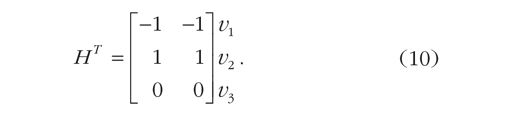
H^{T} = [\begin{matrix} - 1 & - 1 \\ 1 & 1 \\ 0 & 0 \end{matrix}] \begin{matrix} v_{1} \\ v_{2} \\ v_{3} \end{matrix} .

(10)

We then proceed estimating a linear model after defining the contrast matrix $C$ .

Listing 2.1: R code for hypothesis, contrast matrices to estimate regression coefficients in case of highly correlated contrasts

The model’s output clearly shows that one coefficient cannot be estimated because of the high correlation among them that, in turn, determines a singularity. In such cases, the calculation of all the linear model coefficients is impossible. The same applies for their interpretation.

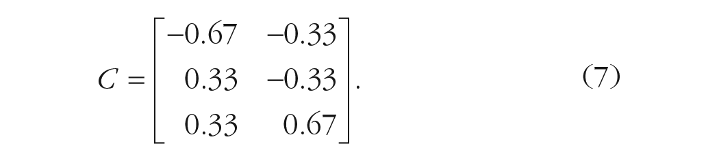
Another consideration is linked to the scale of the contrast weights in both hypotheses and contrast matrices. Consider the contrast weights of Equation 7. Note that the contrast weights produced by the generalized matrix inverse ( $\pm 0.67$ and $\pm 0.33$ ) have a different scale (weight variances) than the weights in $H$ . The scale of the weights in $C$ is important for correctly interpreting the $B$ coefficients obtained from the estimation of the linear model. In the previous example, because the $C$ matrix contains weights that are 1 unit apart (–.67 vs .33), the corresponding $β$ coefficient represents the difference between the mean of $g 2$ and the mean of $g 1$ . If the weights are $k$ units apart, the $β$ coefficient will still represent the difference between the means but scaled by a factor of $1 / k$ .

To provide a concrete explanation, consider Example 1. If the contrast matrix were coded as $(- 1, 1)$ , the $β$ coefficient estimated by the linear model would have been numerically different from the difference between the means of the two groups, that is, $(μ_{2} - μ_{1}) / 2$ . This is because the two levels are 2 units apart, and thus, the $β$ coefficient would have been half the distance between the two means. On the other hand, because $C = (- . 5, . 5)$ was employed, the value of $β$ corresponds exactly to the difference in means. In general, both matrices may have a different scale: The scale necessary to set the initial comparisons being tested is indicated by the $H$ matrix, and the scale of the comparison used in the linear model computations is given by the $C$ matrix. If only inferential tests are of interest, one could argue that the scale is not important.

A final consideration regards the standardization of the coefficients.³ It is well known that in linear models, the standardized coefficients are obtained by estimating the model after standardizing all variables. Thus, to compute the standardized $β$ coefficients, after standardizing the dependent variable, one needs to ensure that the columns of the $C$ matrix have a variance equal to 1. This can be obtained by

Z_{j} = C_{j} / \sqrt{\frac{1}{k} \sum_{i} (c_{j i}^{2})},

(11)

where $Z$ is the standardized $C$ matrix, $j$ is the index of the contrast, and $c_{j i}$ is the ith weight of the jth contrast. As can be easily verified, the $H$ matrix of the standardized contrast matrix is qualitatively equivalent to the one obtained from the original $C$ , that is, the tested comparisons are the same. Using $Z$ as the contrast matrix guarantees that the contrast variable cast in the linear model is standardized, thus producing standardized coefficients when the dependent variable is standardized as well.

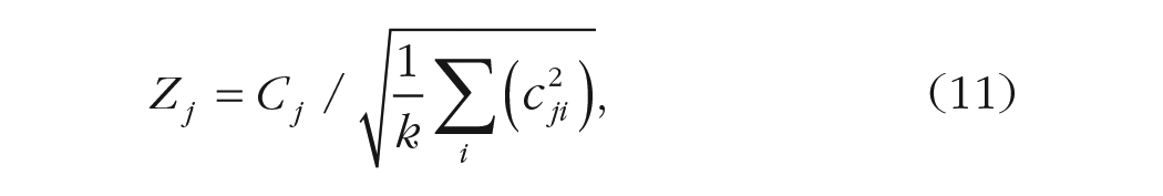
Another form of standardization often used is normalization (Liu, 2013). The aim is to obtain weights whose sum of squares equals $1$ . This allows for comparisons of the size of the contrasts coefficients within and across studies. The normalization is simply as follows:

N_{j} = C_{j} / \sqrt{\sum_{i} (c_{j i}^{2})},

(12)

where $N$ is the normalized contrast matrix.

Type of contrasts

Treatment contrasts

Suppose a researcher has two experimental conditions and wants to compare each of them with a control/placebo condition. In cases such as this, treatment contrasts are the easiest solution. Assuming $k$ levels of a categorical variable, in the case of treatment contrasts (or dummy contrasts), the objective is to compare $k - 1$ levels (coded with the value $1$ ) with a level chosen as a reference, baseline, or control condition (coded with the value $0$ ). Consider a generic variable G ( $k = 3$ levels: $g_{1}, g_{2}, g_{3}$ ). In this case, assuming the level $g 1$ as the reference level (and coded with 0), the planned comparisons would be $g 2$ compared with $g 1$ and $g 3$ compared with $g 1$ .

In the example at hand, the transposed hypothesis and contrast matrices (including the intercept as first column) would be the following⁴:

H^{T} = [\begin{matrix} 1 & - 1 & - 1 \\ 0 & 1 & 0 \\ 0 & 0 & 1 \end{matrix}] C^{T} = [\begin{matrix} 1 & 0 & 0 \\ 1 & 1 & 0 \\ 1 & 0 & 1 \end{matrix}] .

(13)

The first column of the hypothesis matrix provides useful information on this contrast type and the meaning of the intercept in a potential regression model. In case of treatment contrasts, the intercept coincides with the mean of the first group. In terms of hypothesis testing,

H_{0} : μ_{1} = 0 .

(14)

Although not technically a contrast (their weights do not sum up to 0), treatment contrasts are very simple to interpret and represent the default coding system in several statistical software packages, including R (R Core Team, 2021). However, when there are interactions in the model or the intercepts are of interest for the model (as in mixed models), the researcher should be aware that the contrasts weights do not sum up to 0, and thus, the interpretation of the model parameters may be different than expected. In the next paragraphs, the importance of the weights summing up to 0 will be clarified.

Simple contrasts

A commonly used contrast coding scheme is centered-treatment coding, also known as “simple” contrasts. This coding scheme is useful because it retains the same interpretation as treatment-contrasts coding but with the added advantage of being centered, allowing for its use in interactions. The centering here is achieved by setting the intercept to the grand mean. In the example at hand, the transposed hypothesis matrix differs from the contrast matrix only in the intercept coding:

H^{T} = [\begin{matrix} 0.33 & - 1 & - 1 \\ 0.33 & 1 & 0 \\ 0.33 & 0 & 1 \end{matrix}] C^{T} = [\begin{matrix} 1 & - 0.33 & - 0.33 \\ 1 & 0.66 & - 0.33 \\ 1 & - 0.33 & 0.66 \end{matrix}] .

(15)

Thus, as for the treatment contrasts, the first contrast in $C$ (excluding the intercept in the first column) compares $g 2$ and $g 1$ , and the second contrast compares $g 3$ with $g 1$ . This is equivalent to centering⁵ the treatment-contrast matrix $C$ to $1 / k$ .

Deviation contrasts

Suppose a researcher wants to compare the incomes of two specific categories of workers with the average income of the overall workers of a country. In this case, deviation contrasts can be useful. Deviation contrasts, also named “sum” or “effect” contrasts, aim at comparing the $k - 1$ levels with the grand mean of those levels (i.e., the mean of the means). In this example, assuming Level $g 3$ as the reference level, the planned comparisons would be the following: $g 1$ compared with the grand mean and $g 2$ compared with the grand mean.

In the example at hand, the transposed hypothesis and contrast matrices would be

H^{T} = [\begin{matrix} 0.33 & 0.66 & - 0.33 \\ 0.33 & - 0.33 & 0.66 \\ 0.33 & - 0.33 & - 0.33 \end{matrix}] C^{T} = [\begin{matrix} 1 & 1 & 0 \\ 1 & 0 & 1 \\ 1 & - 1 & - 1 \end{matrix}] .

(16)

In this type of contrast, the hypothesis on the intercept (of a potential linear model) states that such a grand mean of the levels is equal to zero:

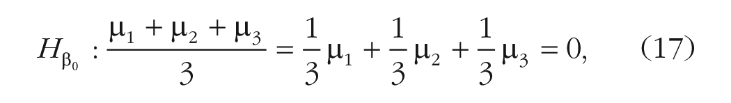
H_{β_{0}} : \frac{μ_{1} + μ_{2} + μ_{3}}{3} = \frac{1}{3} μ_{1} + \frac{1}{3} μ_{2} + \frac{1}{3} μ_{3} = 0,

(17)

where $\frac{1}{3} = 0.33$ are the contrast weights assigned to the intercept column of the hypothesis matrix $H^{T}$ . It follows that the hypothesis on the first contrast can be written as follows:

H_{β_{1}} : μ_{1} = \frac{μ_{1} + μ_{2} + μ_{3}}{3} = \frac{2}{3} μ_{1} - \frac{1}{3} μ_{2} - \frac{1}{3} μ_{3} = 0 .

(18)

It is easy to verify that the second contrast is computing $- \frac{1}{3} μ_{1} + \frac{2}{3} μ_{2} - \frac{1}{3} μ_{3}$ .

Repeated contrasts

Suppose a researcher aims at comparing the level of noise detected among three adjacent urban areas of a city. In particular, the aim is to compare each urban area with its adjacent one. In this case, repeated contrasts can be very useful. In repeated contrasts, also known as “successive-difference contrasts,” “sliding-difference contrasts,” or “simple-difference contrasts,” the aim is to compare the neighboring levels of a variable. For instance, considering again the variable G, if $k = 3$ , the contrasts would be $g 2$ compared with $g 1$ and $g 3$ compared with $g 2$ . In the example at hand, the transposed hypothesis and contrast matrices would be the following:

H^{T} = [\begin{matrix} 0.33 & - 1 & 0 \\ 0.33 & 1 & - 1 \\ 0.33 & 0 & 1 \end{matrix}] C^{T} = [\begin{matrix} 1 & - 0.67 & - 0.33 \\ 1 & 0.33 & - 0.33 \\ 1 & 0.33 & 0.67 \end{matrix}] .

(19)

Polynomial contrasts

Suppose a researcher aimed at comparing the attention skills of three age groups: children, adolescents, and adults. In particular, the researcher has two specific hypotheses: understanding if attention skills can follow a linear trend or a U-shape trend. In this case, polynomial contrasts can be used. Polynomial contrasts, also named “orthogonal-polynomial contrasts,” are useful to test possible trends of the variable’s levels (i.e., linear, quadratic, cubic).

For the variable G with $k = 3$ , the contrasts would be the following: linear, the trend of levels is linear; quadratic, the trend of levels is quadratic. In the example at hand, the transposed hypothesis and contrast matrices would be⁶

H^{T} = [\begin{matrix} 0.33 & - 0.71 & 0.41 \\ 0.33 & 0 & - 0.82 \\ 0.33 & 0.71 & 0.41 \end{matrix}] C^{T} = [\begin{matrix} 1 & - 0.71 & 0.41 \\ 1 & 0 & - 0.82 \\ 1 & 0.71 & 0.41 \end{matrix}] .

(20)

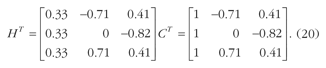
The polynomial contrasts are orthogonal, that is, the correlation between weights is 0 (for a discussion, see below). When the sum of squares of the weights of each contrast is 1, they are named “orthonormal-polynomial contrasts.”

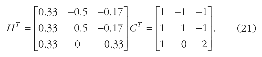
Helmert contrasts

Consider again the previous three age clusters. Now the aim is to understand if the attention skills can be different between (a) children versus adolescents and (b) nonadults (i.e., children and adolescents taken together) versus adults. In this case, Helmert contrasts can be applied.

With Helmert contrasts, it is possible to compare each of the $k - 1$ levels with the average of its previous ones. In the case at hand (e.g., on the variable G), the comparisons would be $g 1$ compared with $g 2$ and the average between $g 1$ and $g 2$ compared with $g 3$ . In the example at hand, the transposed hypothesis and contrast matrices would be

H^{T} = [\begin{matrix} 0.33 & - 0.5 & - 0.17 \\ 0.33 & 0.5 & - 0.17 \\ 0.33 & 0 & 0.33 \end{matrix}] C^{T} = [\begin{matrix} 1 & - 1 & - 1 \\ 1 & 1 & - 1 \\ 1 & 0 & 2 \end{matrix}] .

(21)

Reverse Helmert contrasts

Suppose a data analyst is following three soccer teams, A, B, and C. Suppose this analyst wants to compare the average won competitions of each team with all the other successive teams taken together. Assuming a start with Team A, the researcher wants to compare A with B and C taken together. Likewise, the researcher wants to compare B with C. In this case, reverse Helmert contrasts can be applied.

With reverse Helmert contrasts, it is possible to compare each of the $k - 1$ levels with the average of its following ones. These contrasts consist of the reversed version of the Helmert contrasts. Therefore, considering the previous variable, the comparisons would be $A$ compared with the average of $B$ and $C$ and $B$ compared with $C$ . In the case of a reverse Helmert, transposed hypothesis and contrast matrices would be

H^{T} = [\begin{matrix} 0.33 & 0.33 & 0 \\ 0.33 & - 0.17 & 0.5 \\ 0.33 & - 0.17 & - 0.5 \end{matrix}] C^{T} = [\begin{matrix} 1 & 2 & 0 \\ 1 & - 1 & 1 \\ 1 & - 1 & - 1 \end{matrix}] .

(22)

It can be observed that the hypothesis related to the intercept of designs uses all contrasts types, but treatment contrasts are the same (i.e., the intercept reflects the grand mean of observations and is equal to 0).

General characteristics

Note that all the contrasts except the treatment ones sum up to 0. This is important when the categorical variable coded by the contrast is involved in interactions because this aspect guarantees that the other variable first-order effects may be interpreted as average or main effects (Cohen, 1968). Furthermore, Helmert, reverse Helmert, and polynomial contrasts have another important characteristic: orthogonality. Taking two contrasts $c_{1}$ and $c_{2}$ , whose weights sum up to 0, they are orthogonal if their covariance is 0, that is, if $\underset{k = 1}{\sum^{K}} c_{1, k} \times c_{2, k} = 0$ , where $k$ is the $k$ th contrast weight contained in each cell of the contrast column. Orthogonal contrasts can be advantageous when testing a specific hypothesis. Because they are not correlated, each estimated effect is independent of the other. This implies that they can explain a specific portion of the model’s variance that is not shared with the others. Therefore, their interpretation is more straightforward.

Orthogonality can be useful also when a custom contrast set is defined to test a specific hypothesis. The researcher may aim at testing only one hypothesis even when the categorical variable has $k > 2$ levels, thus requiring $k - 1$ contrasts to properly estimate the model. In these cases, a $C$ matrix can be constructed in such a way that the researcher’s hypothesis is defined and the remaining contrasts are all orthogonal to the one specified by the research (named “filler contrasts”). Orthogonality ensures that the researcher’s hypothesis is not affected by the other contrasts in the model (for a detailed explanation on this issue, see Cohen, 1968). Filler contrasts and in general, orthogonal contrasts are usually constructed by software. In the following sections, we show how to construct and interpret contrasts with ease.

Interactions Contrasts

Interaction terms are products of first-order terms (Aiken & West, 1991), and contrast terms are not an exception. Thus, in a model with more than one categorical independent variable, the interaction terms are coded as the product of the contrasts representing each variable in the interaction.

Example 4

Consider a design with two categorical variables, $A$ and $B$ , both having two levels and coded with deviation coding.

The hypothesis matrix has three columns and four rows: The first column encodes the main effect of A, the second column encodes the main effect of B, and the third column encodes the interaction effect. The four rows correspond to the four conditions’ means (i.e., $μ_{11} = a_{1} b_{1}, μ_{12} = a_{1} b_{2}, μ_{21} = a_{2} b_{1}, μ_{22} = a_{2} b_{2}$ ).

Regarding the main effect of A, the null hypothesis tests whether the average of the two levels of variable A is equal across the levels of variable B:

H_{β_{1}} : (\frac{1}{4} μ_{11} + \frac{1}{4} μ_{12}) - (\frac{1}{4} μ_{21} + \frac{1}{4} μ_{22}) = 0 .

(23)

The use of $\frac{1}{4}$ derives from the same principle as Equation 17, where the coefficients are 1 over the number of conditions.

Regarding the main effect of B, the null hypothesis tests whether the average of the two levels of variable B is equal across the levels of variable A:

H_{β_{2}} : (\frac{1}{4} μ_{11} + \frac{1}{4} μ_{21}) - (\frac{1}{4} μ_{12} + \frac{1}{4} μ_{22}) = 0 .

(24)

Most important, the interaction contrast tests whether the effect of variable A differs across the levels of variable B. In other words, it tests the difference of difference. The null hypothesis is formulated as

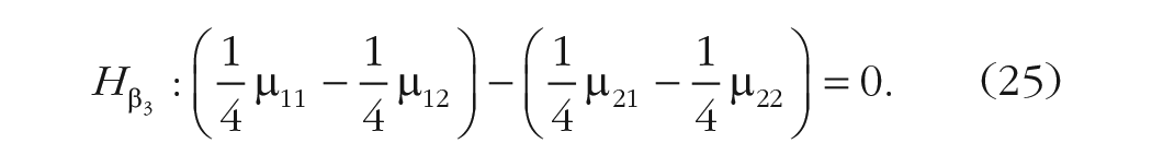
H_{β_{3}} : (\frac{1}{4} μ_{11} - \frac{1}{4} μ_{12}) - (\frac{1}{4} μ_{21} - \frac{1}{4} μ_{22}) = 0 .

(25)

The (transposed) hypothesis matrix in this example (with the index of the combination of levels on the right side and excluding the intercept) would be

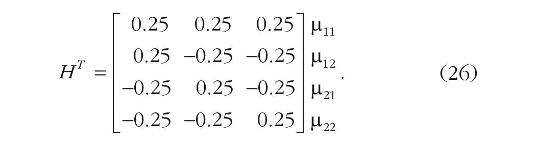
H^{T} = [\begin{matrix} 0.25 \\ 0.25 \\ - 0.25 \\ - 0.25 \end{matrix} \begin{matrix} 0.25 \\ - 0.25 \\ 0.25 \\ - 0.25 \end{matrix} \begin{matrix} 0.25 \\ - 0.25 \\ - 0.25 \\ 0.25 \end{matrix}] \begin{matrix} μ_{11} \\ μ_{12} \\ μ_{21} \\ μ_{22} \end{matrix} .

(26)

By applying the generalized inverse function on $H^{T}$ , the resulting (transposed) contrasts matrix for both main effects and the interaction is

C^{T} = [\begin{matrix} 1 \\ 1 \\ - 1 \\ - 1 \end{matrix} \begin{matrix} 1 \\ - 1 \\ 1 \\ - 1 \end{matrix} \begin{matrix} 1 \\ - 1 \\ - 1 \\ 1 \end{matrix}] \begin{matrix} a_{1} b_{1} \\ a_{1} b_{2} \\ a_{2} b_{1} \\ a_{2} b_{2} \end{matrix} .

(27)

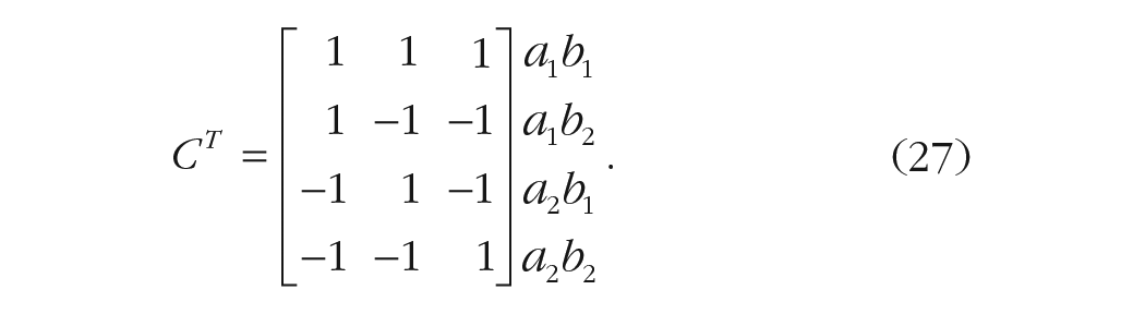
Note that the interaction contrast in $C^{T}$ is the column-wise product of the two former columns, which is indeed the product of deviation coded variables. In fact, the third contrast is testing $(a_{1} b_{1} - a_{1} b_{2}) - (a_{2} b_{2} - a_{2} b_{1})$ , which follows from the very definition of interaction: the difference between the effect of one variable (say $B$ ) at different levels of the other variable ( $A$ in this case). This way of defining interaction contrasts holds independently of the contrasts related to the simple (or main) effects and/or the research design.

In the following section, the appRiori app will be introduced, and its use for the computation and interpretation of contrasts, both for simple effects and for interactions, will be described.

appRiori: organization and functioning

appRiori is a web-based tool coded in the R environment and RStudio (RStudio Team, 2020) using the shiny package (Chang et al., 2021). After downloading and installing R and RStudio, appRiori can be installed by running the install.packages(appRiori) command. Any potential package dependencies, including the shiny package, will be installed simultaneously, or the system will prompt the user to download such dependencies. Once the package is downloaded, it can be loaded by running the library(appRiori) command. Finally, to launch the app, simply run the appRiori() command without inserting any arguments inside the parentheses. A working version of appRiori can be downloaded from CRAN at https://cran.r-project.org/web/packages/appRiori/index.html. It is designed to systematically guide users through this tutorial and all issues related to contrast coding. appRiori is organized into four consecutive panels: introduction, data, single variable, and interactions.

Introduction is the first panel and contains a set of menus. After a quick look at the welcome message, the user can find the “theoretical background” subsection, which provides both the theoretical background and descriptions of contrast types mentioned above. In the following subsection, we provide a guide on how to use appRiori and practical examples.

How appRiori works

After a brief explanation of the contrast coding logic, the introduction panel of appRiori contains a tutorial subsection called “How AppRiori Works,” aimed at guiding the user through the app. This tutorial starts from the second panel of appRiori, called “Data.” This panel allows users to work with the default databases available in their R. Otherwise, users can upload a .csv file containing raw data. Similar to the read.table() function of R, it is possible to set the types of field separator, decimal, and quote. Furthermore, setting the first row as a header is optional. Once the data have been uploaded, appRiori displays them as a data table (Fig. 1, right). Users can select the number of rows displayed and search for specific values through a search bar. Moreover, users can show specific variables by flagging the corresponding box in the “Column to show” list. Finally, a box containing information about the data is displayed at the bottom of the panel; in particular, the type of data (e.g., numeric, float, character, or factor) corresponding to each selected column is explained. As an example, a file called “test.csv” has been uploaded (it can be downloaded from the supplementary material, available at https://doi.org/10.17605/OSF.IO/MQ5AZ), and Columns A and B have been selected (Fig. 1, bottom left). Both columns contain character values, as suggested by the “Data structure” panel of Figure 1.

Fig. 1.

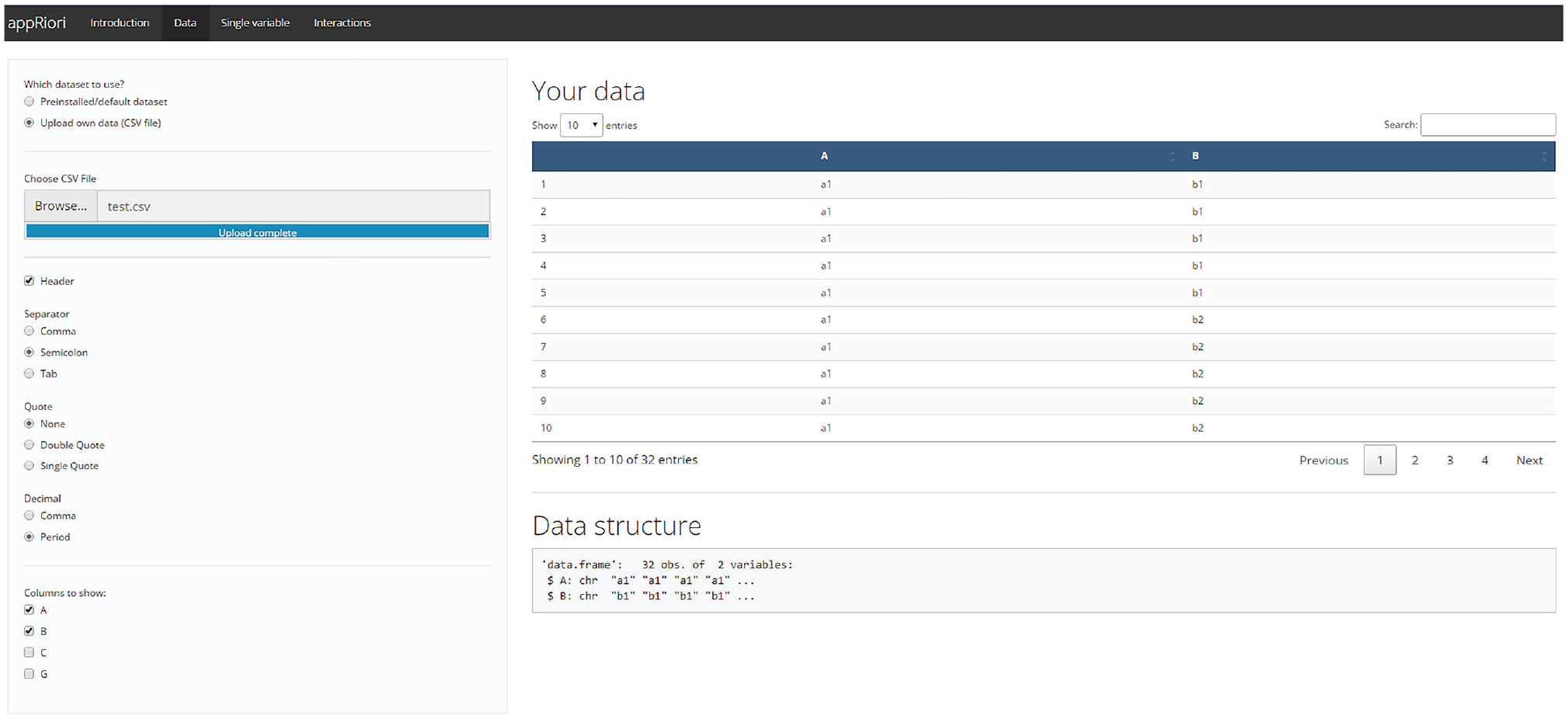
Data section panel.

Once the data have been uploaded, the user can use the last two panels, called “Single variable” and “Interaction.” The third panel allows planning contrasts on a single variable at a time. The fourth panel allows planning contrasts in the case of two- and three-way interaction designs. Both panels are programmed to work with character or factor variables of the selected database. A detailed description of both panels is provided in the following sections.

In general, the user is guided through the comparison planning process through a step-by-step procedure, as shown in Figure 2, that starts from determining which variable(s) will be the target (Step 1) and which kinds of contrasts should be assigned to such variable(s) (Step 2). The user can make such choices by using the corresponding drop-down menus. The variable selection menu is always above the contrast selection menu. Figure 2 shows an example of the appRiori output. In this case, the variable G of the database test.csv has been selected, and repeated contrasts (see the previous subsection) have been assigned to it.

Fig. 2.

Example of appRiori output in case of single variable.

Once the choices are made, appRiori displays the following matrices:

Levels: This matrix shows the original levels that belong to the selected variable (Step 3.0).

Original contrast matrix: This is the default contrast matrix produced in R after converting the selected variable into a factor variable. It corresponds to the contrast(factor()) command (Step 3.0).

New contrast matrix: This is the contrast matrix corresponding to the new hypotheses⁷ (Step 3.0).

Transposed hypothesis matrix: This is a hypothesis matrix in which each row codes one condition, group, or level and each column codes one hypothesis (Step 3.0). appRiori is programmed to provide the easiest set of contrast weights for each comparison to enhance readability of the hypotheses.

A correlation matrix that displays the relationship among the new contrast columns (Step 3.1): This matrix provides information on the orthogonality of the contrasts.

Moreover, appRiori provides a pop-up in which a summary of the user’s selection is described, containing information on how many comparisons can be tested or selected and how the specific contrasts coding scheme works (Step 4). As mentioned above, appRiori allows a researcher to retrieve the code corresponding to the provided output. This code can be obtained inside the “Get your code” section at the bottom of both panels (Step 5). By clicking on the “Submit” button, a snippet of code is displayed that contains (Fig. 2, lower panel) (a) the conversion of the selected variable(s) from character to factor type (by default, appRiori is programmed to convert the target variables into factors) and (b) assignment of the desired contrast matrix to the original one. (c) These two operations can be done in two ways: by using basic R code or using code taken from the hypr package (Rabe et al., 2020). In the latter case, an object is created using the hypr() function; then the new contrast matrix is written inside this object. Finally, the result of this latter code is assigned to the contrasts() function with reference to the target variable(s).

For some modes of the app, appRiori relies on hypr to produce contrast matrices or give the user the option to choose between base R and hypr. Essentially, hypr provides different functions in R to translate between hypothesis and contrast matrices. It is important to stress that appRiori does not intend to replace the functionality of hypr. Actually, appRiori serves at least three complementary purposes. First, appRiori illstruates how hypr aligns with standard contrast functions. Second, appRiori can be used as a graphical interface to get acquainted with the ideas underlying hypr. Third, hypr requires a higher level of proficiency with contrast coding, whereas appRiori is of a more instructional nature.

In brief, with appRiori, one selects the required contrasts and receives the R code necessary to correctly define the contrasts in R scripts. appRiori can handle all the default contrast codings that are available in R. Moreover, it allows the user to define customized contrasts for both single and interaction effects.

Customized contrasts

When the researcher has one or more specific hypotheses that are not encoded in preprogrammed contrast coding, custom contrasts can be defined (Baguley, 2012; Schad et al., 2020). In appRiori, the user can define up to $k - 1$ comparisons. For each comparison, the user can compare two sets of levels or group means. For example, consider the variable N with five levels (i.e., $n_{1}, n_{2}, n_{3}, n_{4}, n_{5}$ ). Assume that the user wants to set the following two comparisons: condition $n_{1}$ against (the average of) all the others taken together (i.e., $n_{1}$ vs $. n_{2}, n_{3}, n_{4}, n_{5}$ ); excluding $n_{1}$ , the (average of) former two conditions with the (average of) latter two (i.e., $n_{2}, n_{3}$ vs $. n_{4}, n_{5}$ ). In appRiori, this kind of customization is handled by creating a series of drag-and-drop menus, as shown in Figure 3.

Fig. 3.

Customized contrast mode.

The user can move each level into one of the two “drop” blocks. Once the comparisons are set, appRiori defines the final contrast matrix by normalizing the customized target contrasts, as shown in the present example:

\begin{array}{r} \begin{matrix} C o n t r a s t 1 : n_{1} \sim (n_{2} + n_{3} + n_{4} + n_{5}) / 4, \\ C o n t r a s t 2 : (n_{2} + n_{3}) / 2 \sim (n_{4} + n_{5}) / 2 . \end{matrix} \end{array}

(28)

Moreover, appRiori adds a group of “filler” contrasts (i.e., coded with the letter “F”; the target contrasts are coded with the letter “T”) that are orthogonal to the target ones. In this way, the final statistical model consumes the necessary degrees of freedom ( $n - 1$ ) that should be expected from the model itself (Cohen, 1968). Filler contrasts are built to be orthogonal to the researcher’s hypothesis, so their values do not affect the tests related to the hypotheses. Finally, appRiori checks that the contrasts set by the user are not linearly dependent; that is, it checks that one of the contrasts is not originated by others. In fact, whenever appRiori identifies a contrast $c_{i}$ that is not linearly independent of the previous ones, it generates a warning message (inside the “Check for linear dependence” section on the left of the panel) notifying that $c_{i}$ is linear dependent and that it will not be coded. Otherwise, the message “Contrasts are linearly independent” is displayed, as in Figure 3.

For the complete list of contrasts coding and how to select them, see Table 2.

Table 2.

Types of Contrasts

Name: default	Name: appRiori	Aim	Notes
Treatment	Treatment	Compare $k - 1$ levels with a baseline level	The reference level is automatically assigned to the first level in alphabetical order. In case of levels coded with alphanumerical strings, the reference will be the one containing the lowest number.
Simple	Simple	Compare $k - 1$ levels with a baseline level	Similar to treatment but centered.
Deviation	Sum	Compare the $k - 1$ levels with the grand mean of those levels	The grand mean will always be assigned to the last level in alphabetical order. In the case of levels coded with alphanumerical strings, the reference will be the one containing the highest number.
Repeated	Sliding difference	Compares neighboring levels
Polynomial	Polynomial	Test possible trends of the variable’s levels (i.e., linear, quadratic, cubic)
Helmert	Helmert	Compare each of the $k - 1$ levels with the average of its previous ones
	Reverse Helmert	Compare each of the $k - 1$ levels with the average of its following ones
	Customized	Customized $k - 1$ comparisons	Available only in appRiori. Checked for linear dependence.

Interactions: default and customized contrasts

In the case of interaction, the definition of planned contrasts is more puzzling. In appRiori, two strategies are provided for handling and customizing interactions.

First, users can select two or three categorical variables (in case a two- or three-way interaction is desired) and set specific contrast matrices for each variable. In appRiori, it is possible to select a specific type of contrast for each variable of interest independently. In all cases, appRiori will provide the final contrast matrix showing how the interaction will be coded in a potential future model. For example, consider the test.csv database and assume that interaction between variables N and A is planned. Moreover, assume the previous customized contrast (Equation 25) for the variable N and the sum contrasts for the variable A. The final contrast matrix (excluding the intercept) is provided in Listing 3.

Listing 3: contrast matrices for interaction (C stands for “Contrast”)

The first two columns (C1 and C2) encode the contrasts related to the main effect of variable N. The third column (C3) encodes the contrasts related to the main effect of variable A. The fourth column (C4) encodes the first contrast of the N variable across the levels of the variable A. This contrast is obtained by multiplying the values in the first and third columns of the contrast matrix. The process is the same for the fifth column (C5). The remaining four columns refer to a set of filler contrasts. It is also possible to customize one or more variables by following the same path described in the previous sections.

Another way to customize contrasts in the case of interactions consists of considering the factorial design as a one-way combination variable, also known as “linearization” of the design. This means that the levels of all variables are combined to define a unique variable with a number of levels equal to the product of the starting variables’ levels. For example, assuming two variables $G$ and $A$ , where the former variable is composed of three levels ( ${g 1, g 2, g 3}$ ) and the latter has two levels ( ${a 1, a 2}$ ), the resulting variable will be composed of six levels (i.e., ${g 1 a 1, g 1 a 2, g 2 a 1, g 2 a 2, g 3 a 1, g 3 a 2}$ ). In appRiori, this strategy is implemented. A new variable called “planned interaction” is generated, composed of the combinations among the levels of the starting variables. Then, the same customization strategy described above for single variables is applied. In this case as well, a collinearity check is performed. Figure 4 shows an example of this option, referred to as the “fully customized design” in appRiori,

Fig. 4.

Example of linearization with appRiori.

Because the linearization option leads to the use of customized contrasts, whenever the final number of comparisons is lower than the possible $n - 1$ comparisons, appRiori adds filler contrasts to guarantee that the necessary degree of freedom of the final model will be consumed (Cohen, 1968). This strategy has the advantage of simultaneously allowing the coding of both simple effects and interaction with a single variable. In this way, it is possible to consider and explain both sources of variance with a single set of levels. This approach is specifically applicable to the general linear model, such as classical factorial ANOVA. However, if the aim is to obtain only an interaction effect, that is, to decompose the degree of freedom of interaction, this last approach is not recommended (Baguley, 2012).

Empirical Examples

In the following subsections, two examples are provided showing how to use appRiori to both plan contrasts and use the obtained code to run statistical analyses.

Example 1

For this example, the anorexia database from the MASS package (Venables & Ripley, 2002) has been used. This database contains data related to the weight change of young female anorexia patients (for further information, type on R console the command “?MASS::anorexia”). It contains the following variables: a categorical variable named “Treat,” referring to therapeutic treatment randomly assigned to each patient (three levels, i.e., Cont [control], CBT [cognitive-behavioral treatment] and FT [family treatment]), and “Prewt,” referring to the weight of the patients before the treatment (in pounds).

Suppose now that a researcher is interested in testing the following hypotheses:

Hypothesis 1: The weight (before treatment) of patients assigned to the control group is not different, on average, from the weight of patients assigned to the other two groups (i.e., receiving CBT or FT).

Hypothesis 2: The weight of patients assigned to the CBT group is not different, on average, from the weight of the patients assigned to the FT group.

The hypotheses can be investigated through customized contrasts in appRiori’s “Single variable” panel. For the first hypothesis, it is possible to select the “Customized” option from the second drop-down menu because this hypothesis corresponds to a reverse Helmert contrast but the default reference does not allow the use of the reverse Helmert option. Because two hypotheses have been proposed, the number of contrasts (coinciding with the maximum number of contrasts that can be set with our variable) is set to 2. As shown in Figure 5, for the first comparison, the Cont level is in the right box, and the other two levels are in the middle box. For the second comparison, the CBT level is in the middle box, and the FT level is in the right box. Finally, both hypotheses will be tested using a linear regression model.

Fig. 5.

Customized contrasts of Example 1.

The code printed by appRiori for this first example would be as shown in Listing 4.

Listing 4: code generated by appRiori for Example 1

After copying and pasting the code and testing the corresponding linear model, the results would be as shown in Listing 5.

Listing 5: linear model of Example 1

In the table of coefficients, the row referring to Treat1 contains the result about the first hypothesis. The difference in pounds, before the study, between the average weight of the participants assigned to the control group and the average weight of participants assigned to the other groups together is $- 1.40$ . This difference is not statistically significant ( $p = . 28$ , last column of the table of coefficients). Therefore, the researcher should fail to reject the null hypothesis, in line with the original hypothesis.

Likewise, the row referring to Treat2 contains the result on the second hypothesis. The difference in pounds, before the study, between the average weight of participants assigned to the CBT group and the average weight of participants assigned to the FT group is $- 0.54$ . This difference is not statistically significant ( $p = . 74$ ). Therefore, the researcher should fail to reject the null hypothesis.

In the case of customized contrasts (or any contrast different from treatment ones), the previous explanation may not be immediately evident from the output provided by the summary() function in R. Therefore, appRriori contains a convenient function called contrasts_summary(), which requires the tested model as an input. As shown in Listing 5.1, this function returns the coefficient table similar to the summary() function, but it specifies which comparisons are tested in the model. In this example, the first row of this output specifies that the Cont level is compared with the weighted mean of the other two levels (i.e., CBT and FT). It is similar to the code inserted as an input in Listing 5, with the difference that the levels are inserted in alphabetical order. Likewise, the second row specifies that the CBT level is compared with the FT level. For each comparison, the expected differences among means, their related standard error, and the statistics and p value are provided. In the case of filler contrasts, contrasts_summary() is programmed not to show them because they should not be considered by default in terms of interpretation (see “customized contrasts” subsection).

Listing 5.1: output of contrasts_summary() function

Example 2

In the second example, a two-way factorial design will be used and involves the airquality database, containing data referring to daily air-quality measurements in New York from May to September 1973. In the current example, the following variables are considered: temp, a numerical variable referring to temperature in Fahrenheit degrees; month, a numerical variable ranging from 1 to 12, where 1 encodes January and 12 encodes December; and day, a numerical variable encoding the days of each month.

Suppose now that a researcher is interested in understanding whether in the second part of 1973 the temperature would change based on the following hypotheses:

Hypothesis 1: The mean temperature in May should be lower than the mean temperature in June. Likewise, the mean temperature in June should be lower than the mean temperature in July. No differences should be observed between the mean temperature of July and August. Finally, the mean temperature in August should be higher than the mean temperature in September.

Hypothesis 2: This set of comparisons should be better detected considering the temperature change that occurs between the first half (which should be warmer) of the month and the second half.

To test such hypotheses, a categorical variable is created that splits each month into two parts. In addition, another variable is coded explicitly stating the name of the month. The following lines of code show how to create and reproduce the data (available in the supplementary material at https://osf.io/mq5az/).

Listing 6: code to reproduce Example 2

After uploading the data and selecting the “Interactions panel,” the “Two way” option is chosen from the first menu. Then month as the first variable and day_bin as the second variable are selected. In terms of coding the contrast, the “sliding difference” option is selected for the first variable, and the option “scaled” is selected for the second variable. Once such selections have been made, the hypotheses are tested through a linear regression (for practical purposes, assume that the response variable called temp is normally distributed).

For this second example, the code representing the choices mentioned above is shown in Listing 7.

Listing 7: code generated by appRiori for Example 2

The results of a model tested after copying and pasting such code within the R console would be as shown in Listing 8.

Listing 8: linear model for Example 2

In the coefficient table, the row referring to Month2-1 contains the comparisons between the mean temperature of June and the mean temperature of May; this difference is equal to $13.54$ and is statistically significant ( $p < . 001$ ). Other statistically significant effects can be observed by comparing the temperatures of both July against June (Month3-2: $B = 4.82$ , $p < . 01$ ) and September against August (Month5-4: $B = - 7.10$ , $p < . 001$ ). No differences emerge when comparing the temperatures of August and July (Month4-3: $B = 0.082$ , $p = . 96$ ).

The row referring to day_bin1 contains the comparison between the mean temperature observed in the first half of the month and the mean temperature observed in the second half of the month. This difference is equal to $3.97$ and is statistically significant ( $p < . 01$ ).

Regarding interaction effects, the row referring to Month2-1:day_bin1 contains the comparisons between the mean temperature of June and the mean temperature of May across the two halves of the month. In other words, the difference in mean temperatures between the two halves of the month of June and those of May is equal to $6.64$ , and it is statistically significant ( $p = . 04$ ). No differences emerge across both July against June (Month3-2:day_bin1: $B = - 5.78$ , $p = . 07$ ) and August against July (Month4-3:day_bin1: $B = 0.91$ , $p = . 77$ ). A statistically significant difference occurs when comparing the two halves of the month of September and those of August (Month5-4:day_bin1: $B = 7$ , $p = . 03$ ).

Example 3

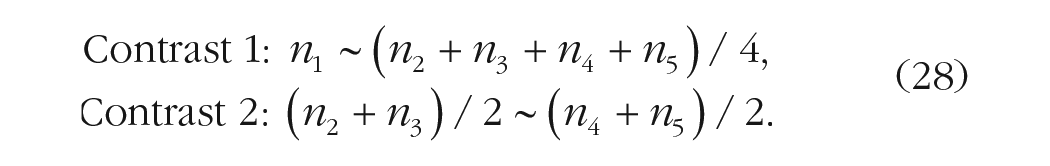
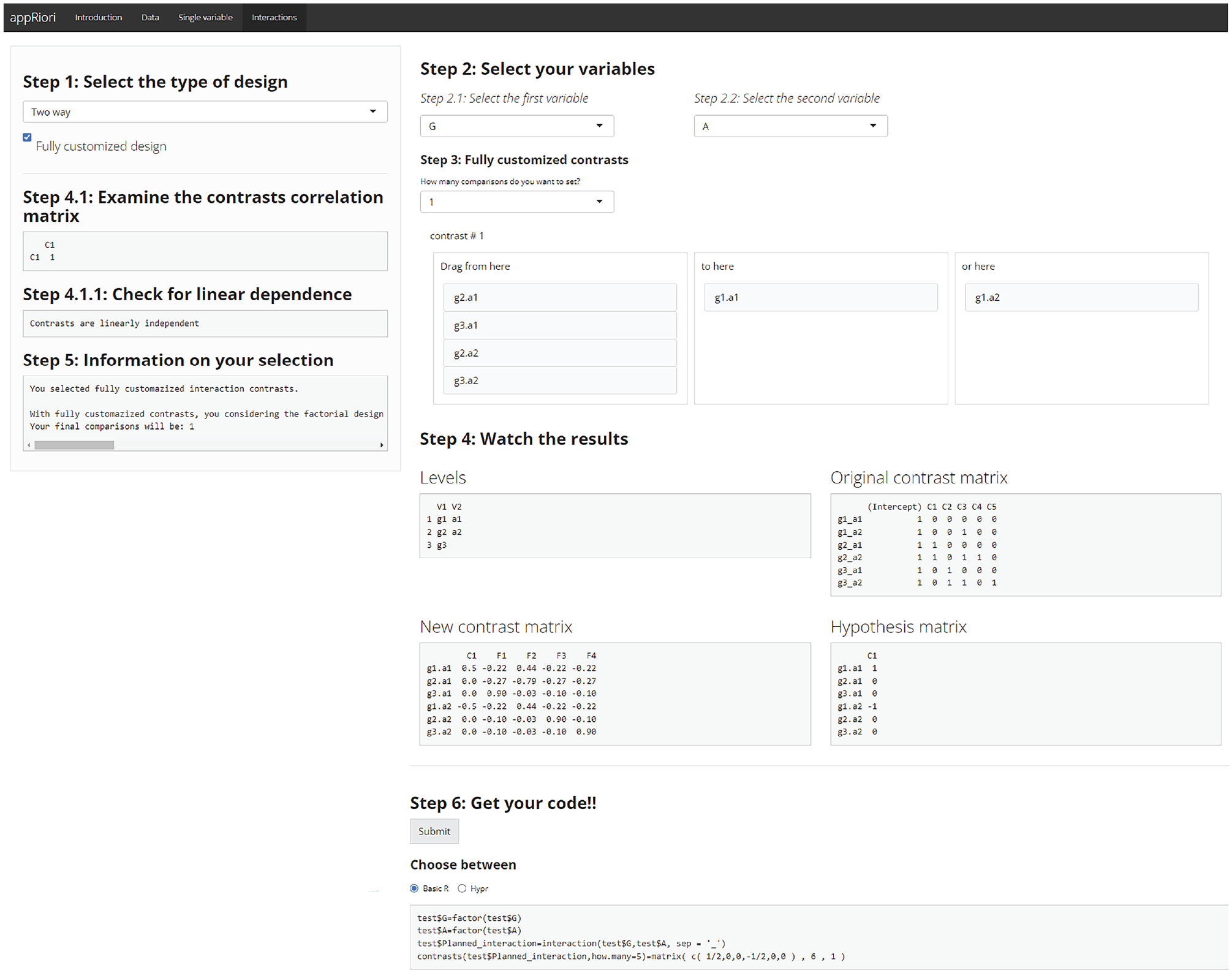
In this last example, the following scenario can be assumed: A group of researchers is replicating a cross-sectional study with a $2 \times 2$ factorial design. Considering both categorical variables they work with (i.e., variable $A$ with levels $a_{1}$ and $a_{2}$ and variable $B$ with levels $b_{1}$ and $b_{2}$ ), the group of researchers wants to test a specific hypothesis. That is, they want to determine if only participants assigned to conditions $a_{1}$ and $b_{1}$ will obtain different scores compared with participants assigned to condition $a_{2}$ and $b_{2}$ . In similar cases, it is possible to use a linearization of the design by creating a new variable composed of four levels (i.e., $a_{1} b_{1}$ , $a_{2} b_{1}$ , $a_{1} b_{2}$ , $a_{2} b_{2}$ ). Note that these data have been created for illustrative purposes and are simulated. The data and script originating from the data are available in the supplementary material. This scenario can be handled in appRiori by selecting the “fully customized” option of the “Interaction” panel. Once this option is selected and the variables are chosen, it is necessary to specify that only one comparison is needed. Figure 6 shows the results of this process.

Fig. 6.

Example of fully customized contrasts, Example 3.

After copying and pasting the code and testing the corresponding linear model, the results would be as shown in Listing 9.

Listing 9: linear model for Example 3

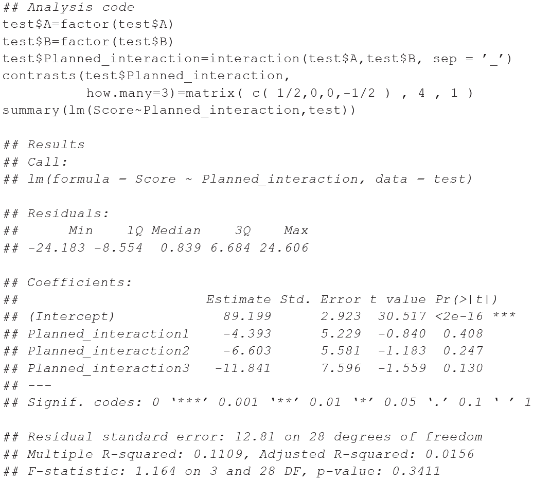
In the coefficient table, the row referring to Planned_interaction1 contains the comparisons between the target groups (i.e., $a_{1} b_{1}$ vs. $a_{2} b_{2}$ ); the expected difference is equal to $- 4.393$ and is not statistically significant ( $p = . 408$ ). Rows referring to Planned_interaction2 and Planned_interaction3 refer to both orthogonal and completely random comparisons made by appRiori that could not be considered.

Summary and Considerations

Several decisions need to be made to represent the comparisons or behaviors of specific patterns/bundles of means in the best way. As Davis (2010) suggested, such decisions can be summarized by a process tree that starts at a primary crossroad: the lack or presence of literature on research hypotheses. Although post hoc (or nonplanned) contrasts can be used, a priori (or planned) contrasts are encouraged. In this branch, a researcher can select between facing trends (e.g., polynomial contrasts) or comparisons between groups of means (Chatham, 1999). Based on the kind of comparisons, the decision will regard the use of orthogonal (e.g., Helmert contrasts) or nonorthogonal contrasts (e.g., treatment or repeated contrasts). Among the possibilities offered by the last categories, researchers sometimes have specific hypotheses that are not covered by the already known contrasts. In such cases, contrast customization is required. Such a process is not trivial: Considering a single variable, the researcher should decide whether it is a case of defining a set of (non)orthogonal contrasts and follow the mathematical principles to encode such characteristics. Researchers need to decide whether contrast weights should be coded by comparing the variable levels of the groups and if so, determine a way to create such groups of levels (Baguley, 2012). This decision process can become more complicated in the case of interactions. During the last 30 years, progress in statistical software and awareness on this topic have increased. It seems that there has been little increase in the use of planned comparisons (Brehm & Alday, 2022; Haans, 2019). Nevertheless, planned contrasts are less preferred than post hoc contrasts, even in the case of nonexploratory studies. A possible reason for this preference (or nonpreference) can be ascribed to the difficulty in understanding, coding, and interpreting planned contrasts. A discussion of the appropriateness of post hoc contrasts or the serendipity they provide (Thompson, 1990) is beyond the scope of this article. In the present work, by introducing the appRiori tool, we try to give an impulse to reduce such difficulties. The advantages of using planned contrasts are several, and there is consensus on this idea that has remained constant over the decades (Davis, 2010; Kuehne, 1993; Schad et al., 2020). In the present tutorial, we try to summarize, in a practical fashion, five main advantages by using a tool like appRiori.

The first aspect pertains to education. Writing about contrasts with strictly formal and methodological language is undoubtedly necessary. Nonetheless, it may hinder researchers from deeply understanding the logic and meaning of contrasts. Post hoc comparisons, on the other hand, are sets of comparisons between pairs of levels. Post hoc comparisons are easier to understand. Therefore, users may be more inclined to use the latter. Even though there are some manuals that are more practical and easier to understand (see e.g., Baguley, 2012), having more tools to help unveil the nature of contrasts can be beneficial.

Recall the misunderstanding about orthogonality: When two or more comparisons are orthogonal, it means that each of them is not a linear combination of the others. To be more specific, they are not even correlated. A clear understanding of this characteristic is of significant importance not only for the explained variance of a model but also for the nontechnical interpretation of specific effects. In general, it is important to prevent comparisons (both planned and post hoc) being used uncritically. As shown throughout the article, the scale of weights of both hypothesis and contrast matrices could not be the same. This influences the final model coefficients. The knowledge of which weights to use to adhere to some target hypotheses may contribute to unveil what happens inside a mathematical black box that is too often not considered. The development of appRiori and its related tutorial followed this spirit: to simplify something that is often considered difficult and therefore, neglected or misused. The introductory panels of the present Shiny app provide the necessary formal basis to understand what a contrast is and why it is important. Moreover, appRiori describes in a user-friendly manner all the default contrasts that can be coded in R software and the ways to interpret them by providing reproducible examples that use easy-to-recall databases in R.

The second advantage concerns contrast customization. Customizing contrasts can not only address general situations in which existing contrasts do not align with researchers’ hypotheses but can also help in encoding very specific hypotheses that can be better interpreted, especially if they are orthogonal (i.e., where all the contrasts are not correlated). In appRiori, users can customize their contrasts using a series of drag-and-drop menus. Specifically, this first version of appRiori is programmed for $n - 1$ pairs of comparisons, and users are required only to drag the desired levels (represented by blocks) into each member of the pair, thereby creating groups of variable levels representing the hypothesized comparisons. The contrasts generated from the app are accurate from a formal point of view, that is, do not exceed the n – 1 comparisons and are not redundant or linearly dependent. Moreover, users can also get an idea of the correlations among comparisons. Finally, the custom contrasts are generated in a way that the scaling of the corresponding hypothesis matrix should be the easiest in terms of readability and interpretation. In this way, the (potential) generated model coefficients can be easily checked and understood. As stated in the section“How to Get Away With Planned Comparisons: A Guide,” the coding is programmed to be coherent with the hypothesis matrix. In other words, if the user wants to directly capture the difference between two conditions, the app is programmed to provide a contrast matrix whose weights are $[0.5, - 0.5]$ , leading to a hypothesis matrix whose weights are $[1, - 1]$ .

A third advantage concerns interactions, in line with the recommendations of previous studies that have delved into the technical aspects of these effects (Garofalo et al., 2022; Rosnow et al., 2000). Beyond planning interaction contrasts and effectively using default contrasts for each variable (in both two- and three-way designs), users can also select the contrasts related to the interaction in two ways. On one hand, they can choose to treat the interaction as a single variable and customize it using the same logic explained in the previous lines; on the other hand, it is possible to customize each variable of the interaction, and appRiori will show how the final contrasts matrix of both simple and interaction effects will look.

The fourth advantage is purely practical because all operations result in generating a set of lines of R code that users can simply copy and paste into their scripts/consoles. This type of output can benefit both beginners and slightly advanced users because the code is written by referring to default R functions and retrieving functions from the hypr package (Rabe et al., 2020). As suggested by Schad et al. (2020), contrast matrices generated by such code could be used not only for analyses of variance but also for linear, generalized (mixed), Bayesian, and nonparametric models.

Finally, the use of a tool capable of helping users to define specific comparisons can help reduce reproducibility issues. Understanding the difference between hypothesis and contrast matrices and the steps necessary to transform one into the other to estimate regression coefficient gives access to information on the background that could remain unused otherwise. As noted in the previous sections, if contrast matrices are passed to the model assuming their contrast weights as identical to the ones of the hypotheses matrices (with the only exception for treatment contrasts), this may lead to coefficients that still allow answering to the research questions, but in a slightly different way. Therefore, the analytic strategy reported in related works could be misleading. When a study does not report the specific strategies adopted to handle comparisons, difficulties in understanding the results may arise. Consequently, it becomes impossible to determine if those results are free from biases or errors, rendering them unreproducible (Brehm & Alday, 2022). The fact that appRiori creates code directly related to the initial hypothesis and that such code can be uploaded to an open-science platform enhances the reproducibility and trustworthiness of the findings.

The proposed tutorial does not solve all the issues related to multiple comparisons. In the case of multiple planned contrasts, the need for correcting the related p values (if p values are used) remains. Nonetheless, the number of comparisons on which it is necessary to adjust definitely decreases compared with the adjustment necessary in the case of post hoc comparisons. Likewise, even the presented web tool is not exempt from limitations. For instance, the customization strategy of the present version of appRiori does not allow the user to define contrast weights directly from raw means or from multiple contrast types. Moreover, interaction contrasts can be coded and/or customized only for two- and three-way factorial designs. If users use the “fully customized” modality (intended as a linearization of the design), it is important to stress that such an approach may not be suitable for other models that capture dependency in the data. Models such as linear mixed models, generalized mixed models, generalized estimating equation, or repeated measure ANOVA may not adhere to the assumption of independence required for the linearization approach to be valid. Each of these limitations provides stimuli for new versions of appRiori. Current works aim to reduce these limitations and make this Shiny app capable of covering a set of cases that is more exhaustive. Beyond the limitations, the implications of using appRiori are twofold. First, this Shiny app is in line with a series of Shiny applications programmed to teach and guide new or old methods for statistical analysis (e.g., see https://shiny.rstudio.com/gallery/) not only related to social sciences. appRiori can be used to teach contrast coding and linear models in matrix algebra to doctoral students and in advanced seminars attended by junior scientists. Second, appRiori can increase the use of planned comparisons, reducing the chance of both Type I and Type II errors and increasing the statistical power of the results.

Footnotes

Acknowledgements

We thank Daniel Schad for the useful insight on programming the shiny App. All the data are available in the cited packages of R or provided at .

Correction (June 2025):

Article updated to correct the equation for the comparison 1 null hypothesis on p. 5.

Transparency

Action Editor: Pamela Davis-Kean

Editor: David A. Sbarra

Author Contributions

Umberto Granziol: Conceptualization; Methodology; Project administration; Software; Supervision; Writing – original draft.

Maximilian Rabe: Methodology; Software; Writing – review & editing.

Marcello Gallucci: Software; Writing – review & editing.

Andrea Spoto: Writing – review & editing.

Giulio Vidotto: Writing – review & editing.

ORCID IDs

Umberto Granziol

Maximilian Rabe

Andrea Spoto

Notes

References

Agathokleous

(2022). Six statistical issues in scientific writing that might lead to rejection of a manuscript. Journal of Forestry Research, 33(3), 731–739.

Aiken

L. S.

West

S. G.

(1991). Multiple regression: Testing and interpreting interactions. Sage.

Baguley

(2012 Serious stats: A guide to advanced statistics for the behavioral sciences. Macmillan International Higher Education.

Brehm

Alday

P. M.

(2022). Contrast coding choices in a decade of mixed models. Journal of Memory and Language, 125, Article 104334. https://doi.org/10.1016/j.jml.2022.104334

Buckless

F. A.

Ravenscroft

S. P.

(1990). Contrast coding: A refinement of ANOVA in behavioral analysis. Accounting Review, 65(4), 933–945.

Chang

Cheng

Allaire

Sievert

Schloerke

Xie

Allen

McPherson

Dipert

Borges

(2021). shiny: Web application framework for r [Computer software manual] (R Package Version 1.7.1). https://CRAN.R-project.org/package=shiny

Chatham

(1999). Planned contrasts: An overview of comparison methods (ED426092). ERIC. https://files.eric.ed.gov/fulltext/ED426092.pdf

Cohen

(1968). Multiple regression as a general data-analytic system. Psychological Bulletin, 70(6, Pt. 1), 426–443. https://doi.org/10.1037/h0026714

Cohen

(1994). The earth is round (p < .05). American Psychologist, 49(12), 997–1003. https://doi.org/10.1037/0003-066X.49.12.997

10.

Davis

M. J.

(2010). Contrast coding in multiple regression analysis: Strengths, weaknesses, and utility of popular coding structures. Journal of Data Science, 8(1), 61–73.

11.

Garofalo

Giovagnoli

Orsoni

Starita

Benassi

(2022). Interaction effect: Are you doing the right thing? PLOS ONE, 17(7), Article e0271668. https://doi.org/10.1371/journal.pone.0271668

12.

Graham

J. M.

(2000). Interaction effects: Their nature and some post hoc exploration strategies (ED438328). ERIC. https://files.eric.ed.gov/fulltext/ED438328.pdf

13.

Haans

(2019). Contrast analysis: A tutorial. Practical Assessment, Research, and Evaluation, 23(9). ERIC. https://files.eric.ed.gov/fulltext/EJ1181418.pdf

14.

Howell

D. C.

(2010). Statistical methods for psychology (7th ed.). Wadsworth Cengage Learning.

15.

Kuehne

C. C.

(1993). The advantages of using planned comparisons over post hoc tests (ED364597). ERIC. https://files.eric.ed.gov/fulltext/ED364597.pdf

16.

Kwon

(1996). The use of planned comparisons in analysis of variance research (ED393916). ERIC. https://files.eric.ed.gov/fulltext/ED393916.pdf

17.

Liu

X. S.

(2013). Statistical power analysis for the social and behavioral sciences: Basic and advanced techniques. Routledge.

18.

Rabe

M. M.

Vasishth

Hohenstein

Kliegl

Schad

D. J.

(2020). hypr: An r package for hypothesis-driven contrast coding. Journal of Open Source Software, 5(48), Article 2134. https://doi.org/10.21105/joss.02134

19.

R Core Team. (2021). R: A language and environment for statistical computing [Computer software manual]. https://www.R-project.org/

20.

R Core Team (2024). An introduction to R. https://cran.r-project.org/doc/manuals/r-release/R-intro.html.

21.

Rosenthal

Rosnow

R. L.

Rubin

D. B.

(1999). Contrasts and effect sizes in behavioral research: A correlational approach. Cambridge University Press.

22.

Rosnow

R. L.

Rosenthal

Rubin

D. B.

(2000). Contrasts and correlations in effect-size estimation. Psychological Science, 11(6), 446–453.

23.

RStudio Team. (2020). Rstudio: Integrated development environment for r [Computer software manual]. http://www.rstudio.com/

24.

Ruxton

G. D.

Beauchamp

(2008). Time for some a priori thinking about post hoc testing. Behavioral Ecology, 19(3), 690–693.

25.

Schad

D. J.

Vasishth

Hohenstein

Kliegl

(2020). How to capitalize on a priori contrasts in linear (mixed) models: A tutorial. Journal of Memory and Language, 110, Article 104038. https://doi.org/10.1016/j.jml.2019.104038

26.

Seaman

M. A.

Levin

J. R.

Serlin

R. C.

(1991). New developments in pairwise multiple comparisons: Some powerful and practicable procedures. Psychological Bulletin, 110(3), 577–586. https://doi.org/10.1037/0033-2909.110.3.577.

27.

Thompson

(1990). Planned versus unplanned and orthogonal versus nonorthogonal contrasts: The neo-classical perspective (ED318753). ERIC. https://files.eric.ed.gov/fulltext/ED318753.pdf

28.

Venables

W. N.

Ripley

B. D.

(2002). Modern applied statistics with s (4th ed.). Springer. https://www.stats.ox.ac.uk/pub/MASS4/

29.

Westfall

P. H.

Young

S. S.

(1993). Resampling-based multiple testing: Examples and methods for p-value adjustment (Vol. 279). John Wiley & Sons.

Not Another Post Hoc Paper: A New Look at Contrast Analysis and Planned Comparisons

Abstract

Keywords

How to Get Away With Planned Comparisons: A Guide

(Brief) Theoretical background

Example 1

Listing 1: R code for hypothesis and contrast matrices to estimate regression coefficients starting from data of Table 1

The importance of the contrast matrix

Example 2

Listing 2: R code for hypothesis and contrast matrices to estimate regression coefficients in case of repeated contrasts

Some clarifications

Example 3

Listing 2.1: R code for hypothesis, contrast matrices to estimate regression coefficients in case of highly correlated contrasts

Type of contrasts

Treatment contrasts

Simple contrasts

Deviation contrasts

Repeated contrasts

Polynomial contrasts

Helmert contrasts

Reverse Helmert contrasts

General characteristics

Interactions Contrasts

Example 4

appRiori: organization and functioning

How appRiori works

Customized contrasts

Interactions: default and customized contrasts

Listing 3: contrast matrices for interaction (C stands for “Contrast”)

Empirical Examples

Example 1

Listing 4: code generated by appRiori for Example 1

Listing 5: linear model of Example 1

Listing 5.1: output of contrasts_summary() function

Example 2

Listing 6: code to reproduce Example 2

Listing 7: code generated by appRiori for Example 2

Listing 8: linear model for Example 2

Example 3

Listing 9: linear model for Example 3

Summary and Considerations

Footnotes

Acknowledgements

Correction (June 2025):

Transparency

ORCID IDs

Notes

References