
Abstract
Meta-analysis is a powerful tool to combine evidence from existing literature. Despite several introductory and advanced materials about organizing, conducting, and reporting a meta-analysis, to our knowledge, there are no introductive materials about simulating the most common meta-analysis models. Data simulation is essential for developing and validating new statistical models and procedures. Furthermore, data simulation is a powerful educational tool for understanding a statistical method. In this tutorial, we show how to simulate equal-effects, random-effects, and metaregression models and illustrate how to estimate statistical power. Simulations for multilevel and multivariate models are available in the Supplemental Material available online. All materials associated with this article can be accessed on OSF (https://osf.io/54djn/).
If you do not simulate it, you have not understood it.
A meta-analysis is an essential tool for combining knowledge from multiple studies quantitatively. Meta-analysis is commonly used together with a systematic review of the literature. The meta-analysis has several advantages. First, it allows combining evidence from multiple studies, assigning more weight to studies with lower estimation variability. Then using metaregression, it is possible to include variables (i.e., moderators) to explain the observed heterogeneity (Borenstein et al., 2009, pp. 187–203). More recently, location-scale models have been developed to include predictors also on the residual heterogeneity (i.e., Viechtbauer & López-López, 2022). Finally, given the replication crisis, there are statistical methods to determine the presence and extent of the publication bias. Despite the advantages, meta-analysis implementation is not always straightforward, especially for complex data structures. In addition, even though there are several introductory and advanced resources to understand meta-analysis (Borenstein et al., 2009; Harrer et al., 2021; Schmid et al., 2022), to our knowledge, there are no introductory resources about how to simulate realistic meta-analytic data.
Simulating data has several advantages because it requires understanding the statistical method and the data-generation process. Furthermore, data simulation is the primary tool when it comes to evaluating a new analysis method, estimating the statistical power, or understanding the long-run behavior of one’s data-generation process (Gelman et al., 2020, pp. 69–76; Gelman & Hill, 2006, pp. 155–176; Ingalls, 2011). A recent article by DeBruine and Barr (2021), which deeply inspired the current work, proposed a stimulating way to understand linear mixed-effects models via data simulation. Simulating data is also a powerful educational tool within this framework.
For these reasons, in this work, we aim to introduce the basic concepts of meta-analysis and Monte Carlo simulations for equal-effects, random-effects, and metaregression models with applications also to statistical power calculation. In the first section, we introduce basic concepts of the meta-analysis that are useful for setting up the simulation. We evaluate the effect size, variance calculation, and the equal- versus random-effects-model distinction. Then we describe how to simulate data for these models and simulate a metaregression with categorical and numerical predictors. Finally, we introduce the power analysis extending the previous examples to estimate the statistical power. We used the R statistical programming language (Version 4.3.1; R Core Team, 2023).
The aim of the tutorial is not to provide a complete theoretical introduction to meta-analysis but, rather, to present core topics using a simulation-based approach. Readers experienced in conducting meta-analyses can benefit from the proposed approach in terms of simulation setup and coding strategies. Readers without prior experience in meta-analysis can benefit from both the theoretical introduction and the simulation approach. However, for a more comprehensive overview of meta-analysis topics, the reader may refer to meta-analysis textbooks (e.g., Borenstein et al., 2009; Harrer et al., 2019).
We assume the reader is familiar with the basic concepts of R, but core functions will be explained. Code and materials are available on the OSF repository (https://osf.io/54djn/). For a theoretical introduction, simulation examples for multivariate and multilevel models, and more details about the coding approach, see the Supplemental Material available online.
Meta-Analysis Introduction
The meta-analysis is a statistical procedure to combine multiple studies (i.e., “primary studies”) into a single statistical analysis (Borenstein et al., 2009). The idea is that combining numerous preliminary studies improves the estimation of a particular phenomenon more efficiently compared with conducting a single study. In statistical terms, the concept of the meta-analysis is to switch the statistical unit from the single participant or observation (i.e., “Level 1”) to the study (i.e., “Level 2”). Given that some studies give more information because their estimation variability is smaller (e.g., higher sample size), the meta-analysis combines the studies, assigning more weight as a function of the precision (i.e., the inverse of the variance).
As an example that will be used throughout the article, we consider the efficacy of memory training in improving memory performance during a cognitive task. The typical primary study will collect data from a group of participants receiving the memory training (“experimental group”) and another group receiving a control treatment (“control group”). The focus of the meta-analysis is collecting multiple studies with similar aims and methods and estimating the average effect of memory training. Despite differences in the type of cognitive task or experimental setup, each primary study collects an experimental group (
Effect Size and Variance
The first step of a meta-analysis is to extract information from included studies. This common measure should give an immediate idea of the direction (i.e., the treatment improves or reduces performance) and the size of the effect. Standardized effect-size measures (for an overview, see Lakens, 2013), such as the standardized mean difference, which could be estimated by Cohen’s
As reported in the previous section, beyond the effect size of each study, one needs to assign a weight according to the precision. For this reason, one needs to calculate the sampling variability of the effect size or the raw measure that will represent the estimation precision. Each raw or standardized effect-size measure (e.g., raw mean difference, Cohen’s
Equal- Versus Fixed- Versus Random-Effects Model
The core of a meta-analysis is combining the results of multiple studies, giving more weight to studies that provide a more precise effect estimation. Essentially, there are three meta-analysis models: the equal-effects, the fixed-effects, and the random-effects model (Hedges & Vevea, 1998; Laird & Mosteller, 1990). The equal-effects model assumes that each study included in the meta-analysis is a more or less precise estimation of the true underlying effect (θ). In other terms, one is assuming that there is no variability (i.e., heterogeneity) among true effect sizes. On the other side, suppose some study-level characteristics (e.g., participants’ age, sex, or socioeconomic status) or the experimental paradigm (e.g., type of memory task or difficulty) could affect the treatment effect. In this case, there is true variability (i.e., heterogeneity) among studies. The random-effects model assumes a distribution of real effects with mean μθ and variance
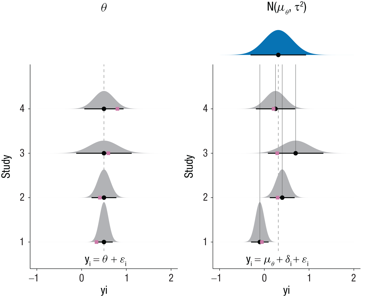
The difference between the assumptions of the equal- and random-effects models. Each distribution depicts the sampling distribution of
Simulation
Monte Carlo simulations
The Monte Carlo methods are controlled experiments (Gentle, 2009). Given a set of fixed parameters, probability distributions, and the possibility of generating random numbers, it is possible to simulate the behavior of an empirical system. Monte Carlo simulations are used for statistical and mathematical problems that cannot be solved analytically.
A straightforward example regards estimating the sampling variability of the mean difference. When calculating the mean difference between two samples, one estimates the true mean difference at the population level with a certain degree of error (i.e., the standard error of the mean difference). The central-limit theorem states that the difference between the means of two random samples (
Generate two random samples from two normal distributions with a fixed mean difference.
Calculate the mean difference.
Repeat the same process many times.
Calculate the standard deviation of the simulated values.
Using the method, one is estimating via simulation the standard deviation of the sampling distribution of the mean difference (i.e., the standard error of the mean difference). Increasing the number of simulations will produce more stable results:

The standard error estimated solving analytically is 0.26, and using the Monte Carlo simulation, one arrives at the same result (i.e., 0.26).
Simulation setup
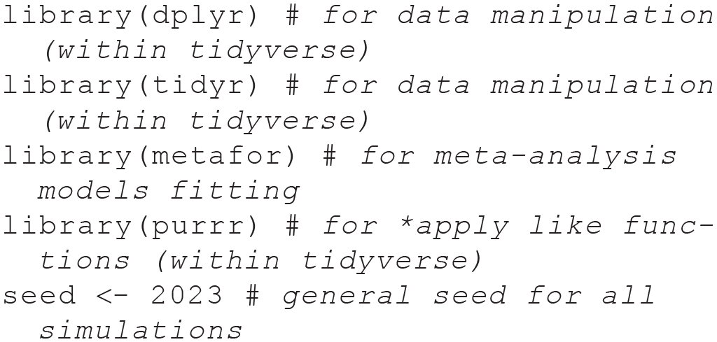
This tutorial uses several R packages for the simulations, meta-analysis fitting, and figures/tables. For the data manipulation, we used the tidyverse (Wickham, 2023) package. For the models fitting, we used the metafor (Viechtbauer, 2010) package. For figures and tables, we used the ggplot2 (Wickham et al., 2023) or the
Before diving into the specific simulations, in this section, we define the common aspects of all simulations in the following sections. In the current article, we focus on the two-level, equal-effects and random-effects models. All the examples refer to primary studies that assess the efficacy of a treatment by comparing a control and an experimental group. In simulation studies in which the purpose is not evaluating effect-size estimators, it is convenient to simulate unstandardized effect-size measures (see Viechtbauer, 2005, 2007). The estimator is unbiased, thus not requiring small-sample correction (Hedges, 1981, 1989). Furthermore, the effect size and the sampling variance are independent. Similar to the simulation approach by Viechtbauer (2005, 2007), the experimental group (


We can use the following algorithm implemented in the
Example of Data Generated With the

Note: The id column is the identifier for each study. nt = number of participants in the experimental and control group; nc = number of participants in the experimental and control group; es = effect size.
Choose a
Simulate
Calculate the observed effect size
The simulation approach can be easily extended to calculating a standardized effect-size measure (e.g., Cohens’

The
The following code simulates a single study with

The control group has a mean of −0.008 (SD = 0.996), and the experimental group has a mean of 0.306 (SD = 1.013), which are remarkably close to the simulated values.
Using the

Variables in the Data-Generating Model and Associated R Code

Note: The yi and vi notation for the observed effect size
Equal-effects model
The most basic model to simulate is the equal-effects model. As reported in the previous sections, the equal-effects model assumes the presence of a single true effect (


Each observed effect size
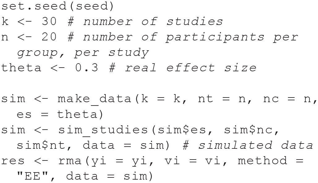
We are using the
Summary of the Simulated Equal-Effects Model

Note: The only estimated parameter is the average effect
Increasing the sample size for each study will increase the estimation precision; thus, the variability among studies will be reduced. This can be easily demonstrated by simulating studies with a high sample size, as reported in Figure 2. As the sample size increases, the only source of variability (i.e., the error component

Forest plots of two simulated equal-effects models. On the left, the simulated model has
Random-effects model
The random-effects model can be considered an extension of the equal-effects model. The equal-effects model assumes that the real effect is a single value. The random-effects model relaxes this assumption, allowing the true effect size to vary across studies. For example, the difference between groups we are simulating could be influenced by the type of experiment or the participants’ age. Now,


Compared with the equal-effects model, we need to generate another adjustment to the overall effect

Then we can fit the random-effects meta-analysis model with the
Summary of the Simulated Random-Effects Model

Note: Compared with the equal-effects model, there are more parameters. The
An important aspect of the random-effects model is the interplay between the heterogeneity

Forest plots of two simulated random-effects models. On the left, the simulated model has
The relationship between the sampling error and the heterogeneity can be expressed using the


From Equation 8 and Figure 3, it is clear that if each included study has a considerable sample size, the sampling variability
Given the interpretation of
Table 5 depicts the results of the random-effects model fixing the
Summary of the Random-Effects Model Fixing the

Note: The β is the average effect (mθ)with the standard error, 95% confidence interval, and the Wald z test. The t2 is the estimated heterogeneity, and the I 2 (explained in the Random-Effects Model section) represents the percentage of total variability due to between-studies heterogeneity. CI = confidence interval.


Metaregression
From a linear-regression perspective, both the equal-effects and the random-effects models can be seen as intercept-only models in which only the mean (i.e., the linear regression intercept) is estimated. As reported in the meta-analysis introduction, the between-studies heterogeneity usually represents the true variability of the effect due to differences among primary studies. A natural extension of the intercept-only analysis is a model that includes variables (i.e., moderators) that could explain the observed heterogeneity among effect sizes. For example, a group of studies could use a particular memory task in which the expected effect is higher than another. In this way, considering the type of task will explain part of the observed heterogeneity, as in standard regression models. Figures 4 and 5 depict a random-effects metaregression model for a categorical and numerical predictor.

Graphical representation of a random-effects metaregression model with a categorical predictor (Condition A and Condition B). Each gray distribution represents the sampling distribution of included studies. The dotted line is the average effect (i.e., random-effects model without moderators). The effect size differs between Conditions A and B, including the condition moderator, explaining part of the total heterogeneity (pink plus green segments). The green segments depict the explained heterogeneity, and the pink segments depict the residual (unexplained) heterogeneity. The pink squares are simulated observed effect sizes from the sampling distributions.

Graphical representation of a random-effects metaregression model with a numerical predictor (
Metaregression with a categorical moderator
A common example of metaregression is by including a categorical predictor, including information about study-level features. In our example, a group of studies uses an online memory task, whereas others use a standard lab-based task. Equation 5 can be easily extended for a metaregression model by including a variable encoding the type of task (online vs. lab-based) and the expected difference between the two levels of the moderator (i.e., the lab vs. online effect). In regression terms (see Equation 11), we could use a dummy variable (


We can simulate the same scenario of the random-effects model with

Now we can fit the metaregression model with the
Summary of the Random-Effects Model With a Categorical Predictor (Lab vs. Online Experiments)
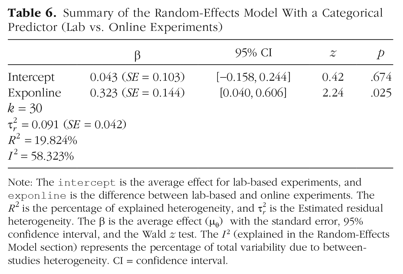
Note: The
Metaregression with a numerical moderator
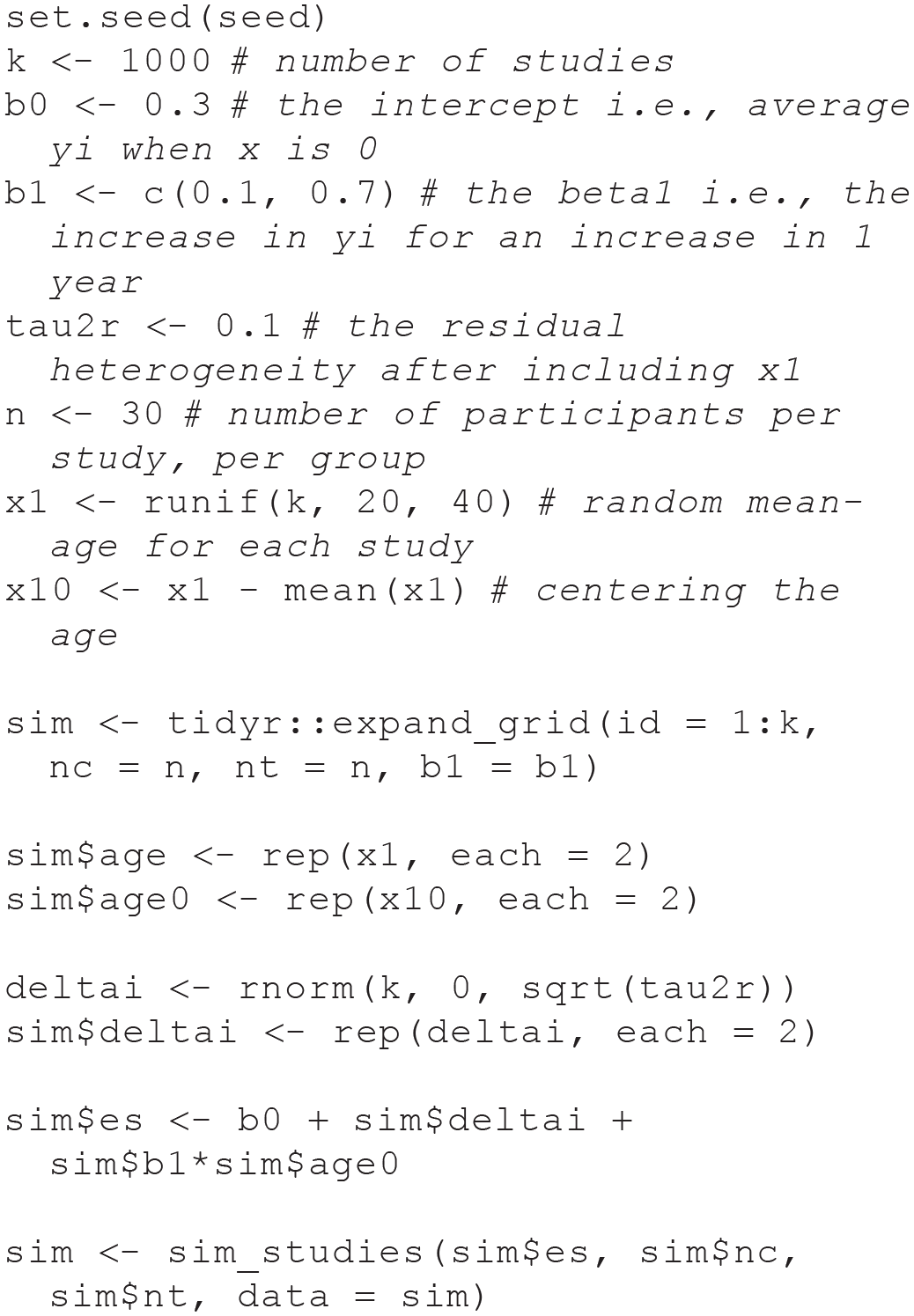
The same approach can be used for a continuous predictor. For example, we can simulate that the average participant’s age within each study could explain part of the observed heterogeneity. Now,

In terms of regression parameters, now the intercept
Assessing the impact of
As reported in the previous section, a strategy to guess plausible values for

Scatter plots with marginal histograms for the range of simulated
Simulating using
A more intuitive way to simulate a continuous predictor is fixing the desired


Now, we can simulate the regression model using

Summary of the Random-effects Model Fixing the
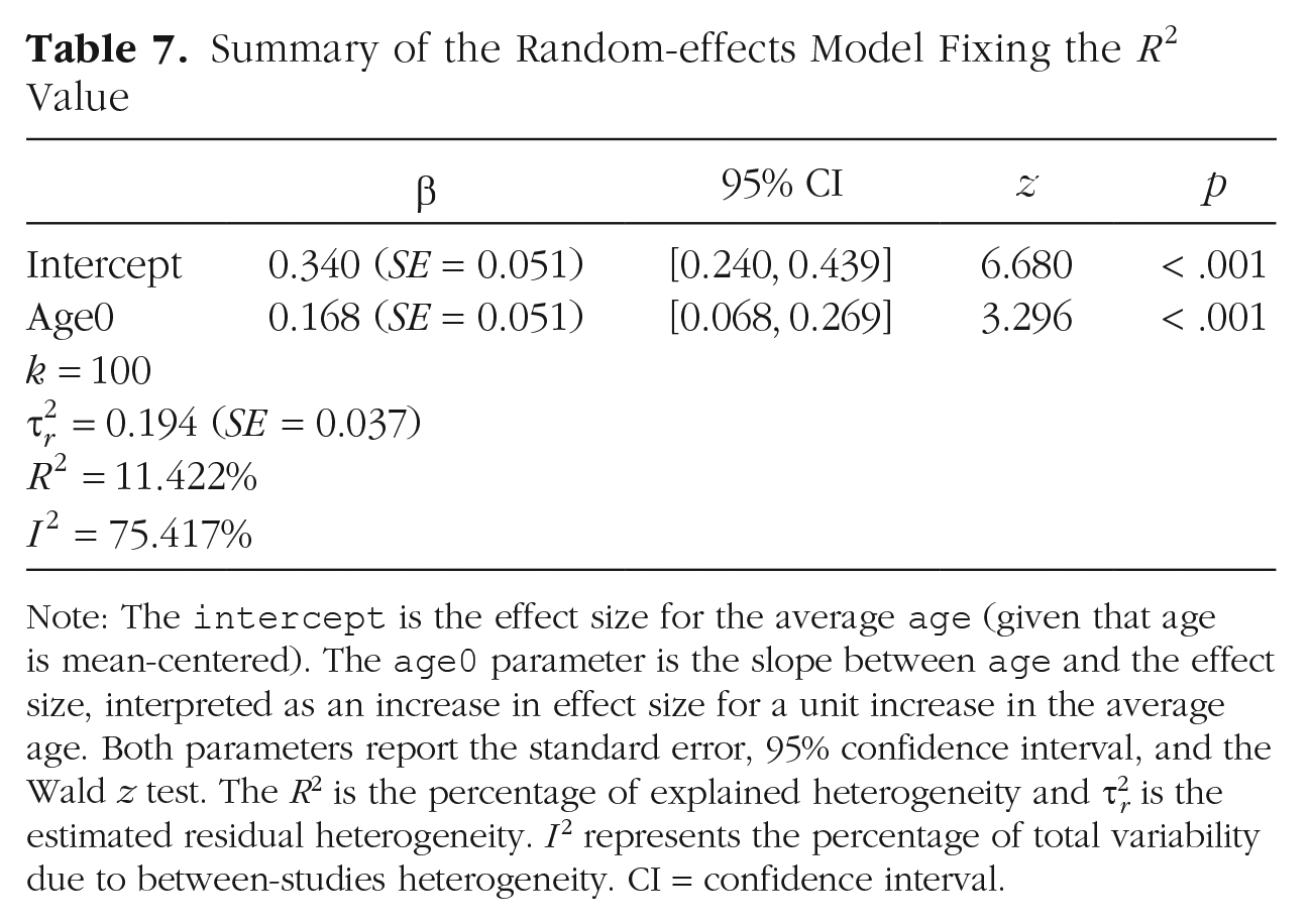
Note: The
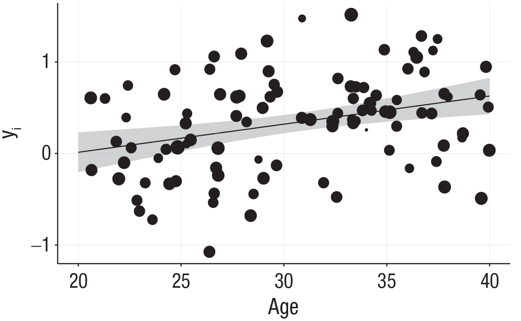
Metaregression results for the random-effects model with a numerical moderator. Each effect size is represented with a black dot where the dimension represents the weight according to the inverse of the variance. The line represents the estimated metaregression slope with the 95% confidence interval (gray bands).
Power Analysis
The previous simulation examples can be easily implemented for multiple purposes. For example, we can use different effect sizes and variance estimators when using the
As explained in the introduction, there are several approaches and tools to estimate the power of equal- and random-effects models (see Borenstein et al., 2009, Chapter 29; Harrer et al., 2019, Chapter 14). These methods are easy to implement but made strong assumptions, such as the homogeneity of sample size, and did not consider the uncertainty in estimating
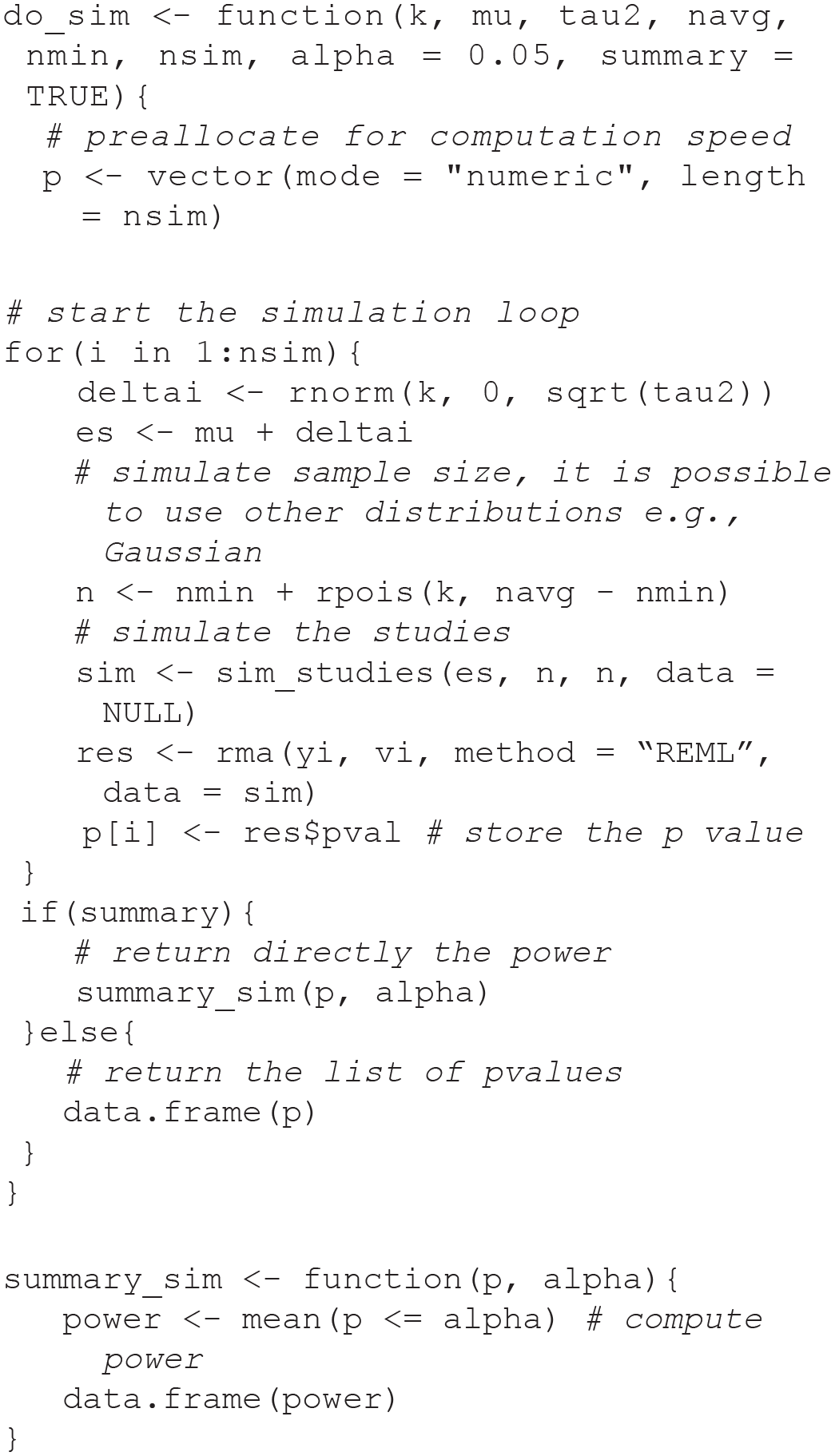
A general Monte Carlo simulation for the power analysis can be implemented with the following steps:
Choose the model that generates the data (e.g., equal- or random-effects model).
Fix the relevant parameters (e.g.,
Simulate a data set.
Fit the appropriate model.
Store the p value associated with the parameter of interest.
Repeat Steps 3 to 5 a large number of times (e.g., 10,000).
Calculate the power as the proportion of p values below the
For example, we can estimate the power of a random-effects model by repeating the simulation presented in the Random-Effects Model section many times. We simulated heterogeneity of sample sizes by sampling
Simulation results are presented in Figure 8 and Table 8 showing that to reach 80% power (usually considered an appropriate level) with a = 0.05 we need ~35 studies. The same approach could be used to estimate the power of a meta-regression by simply modifying the do_sim() function simulating the effect of a moderator and extracting the relevant p-value.

Results from the random-effects model power analysis. The x-axis depicts the number of studies (
The Results From the Power Analysis Simulation

Note: The table depicts the simulation parameters, the estimated power using the

Conclusions
In the present work, we introduced the basic concepts of the meta-analysis regarding equal-effects, random-effects, and metaregression models with a simulation-based approach. We believe the presented examples are useful to implement alternative or more complex models. For example, the
The present work did have a few limitations. First, we introduced only basic concepts about meta-analysis and Monte Carlo simulations, whereas setting up complex simulations requires more knowledge and complexity of the simulation setup. We decided to give the foundations to understand meta-analyses with a simulation approach because more complex models are still based on the same principles. Second, there are limitations concerning simulating participant-level data. We decided to simulate the meta-analysis data starting from the participant level to maximize the flexibility and clearness of each step. The downside concerns the efficiency and scalability of the simulation setup. For large-scale simulations (e.g., many conditions, iterations, or complex models), simulating from aggregated statistics is probably more efficient (for an example, see Heuvel et al., 2020) to improve the simulation efficency. 13
In conclusion, data simulation is a very powerful tool for each step of a data-analysis process, starting from the learning phase, in which simulating data can be used to understand the statistical model in terms of assumptions and the data-generation process, to the estimation of statistical power. Moreover, we believe that data simulation as part of a standard research workflow could improve overall research quality. Data simulation requires understanding the statistical model, setting appropriate and reasoned parameters, and realizing how the chosen analysis method behaves across different scenarios.
Supplemental Material
sj-pdf-1-amp-10.1177_25152459231209330 – Supplemental material for Understanding Meta-Analysis Through Data Simulation With Applications to Power Analysis
Supplemental material, sj-pdf-1-amp-10.1177_25152459231209330 for Understanding Meta-Analysis Through Data Simulation With Applications to Power Analysis by Filippo Gambarota and Gianmarco Altoè in Advances in Methods and Practices in Psychological Science
Footnotes
Acknowledgements
We thank the R-sig-meta-analysis mailing-list. Their suggestions and clarifications significantly improved the simulations approach and the R code. The manuscript preprint was uploaded on PsyArXiv https://psyarxiv.com/br6vy/. Supplementary materials and the code to reproduce simulations, figures, and tables are available at https://osf.io/54djn/ and ![]() .
.
Transparency
Action Editor: Yasemin Kisbu-Sakarya
Editor: David A. Sbarra
Author Contributions
Notes
References
Supplementary Material
Please find the following supplemental material available below.
For Open Access articles published under a Creative Commons License, all supplemental material carries the same license as the article it is associated with.
For non-Open Access articles published, all supplemental material carries a non-exclusive license, and permission requests for re-use of supplemental material or any part of supplemental material shall be sent directly to the copyright owner as specified in the copyright notice associated with the article.