A Guide for Calculating Study-Level Statistical Power for Meta-Analyses

Abstract

Meta-analysis is a popular approach in the psychological sciences for synthesizing data across studies. However, the credibility of meta-analysis outcomes depends on the evidential value of studies included in the body of evidence used for data synthesis. One important consideration for determining a study’s evidential value is the statistical power of the study’s design/statistical test combination for detecting hypothetical effect sizes of interest. Studies with a design/test combination that cannot reliably detect a wide range of effect sizes are more susceptible to questionable research practices and exaggerated effect sizes. Therefore, determining the statistical power for design/test combinations for studies included in meta-analyses can help researchers make decisions regarding confidence in the body of evidence. Because the one true population effect size is unknown when hypothesis testing, an alternative approach is to determine statistical power for a range of hypothetical effect sizes. This tutorial introduces the metameta R package and web app, which facilitates the straightforward calculation and visualization of study-level statistical power in meta-analyses for a range of hypothetical effect sizes. Readers will be shown how to reanalyze data using information typically presented in meta-analysis forest plots or tables and how to integrate the metameta package when reporting novel meta-analyses. A step-by-step companion screencast video tutorial is also provided to assist readers using the R package.

Keywords

meta-analysis statistical power R package

Statistical power is the probability that a study design and statistical test combination can detect hypothetical effect sizes of interest. An a priori power analysis is often used to determine a sample-size (or observation number) parameter using three other parameters: a desired power level, hypothetical effect size, and alpha level. Because any one of these four parameters is a function of the remaining three parameters, statistical power can also be calculated using the parameters of sample size, alpha level, and hypothetical effect size. It follows that when holding alpha level and sample size constant, statistical power decreases as the hypothetical effect size decreases. Therefore, one can compute the range of effect sizes that can be reliably detected (i.e., those associated with high statistical power) with a given sample size and alpha level. For instance, a study design with sample size of 40 and an alpha of .05 (two-tailed) that uses a paired samples t test has an 80% chance to detect an effect size of 0.45 but has only a 50% chance of detecting of an effect size of 0.32 (Fig. 1). In other words, this study design and test combination would have a good chance of missing effect sizes smaller than 0.45.

Fig. 1.

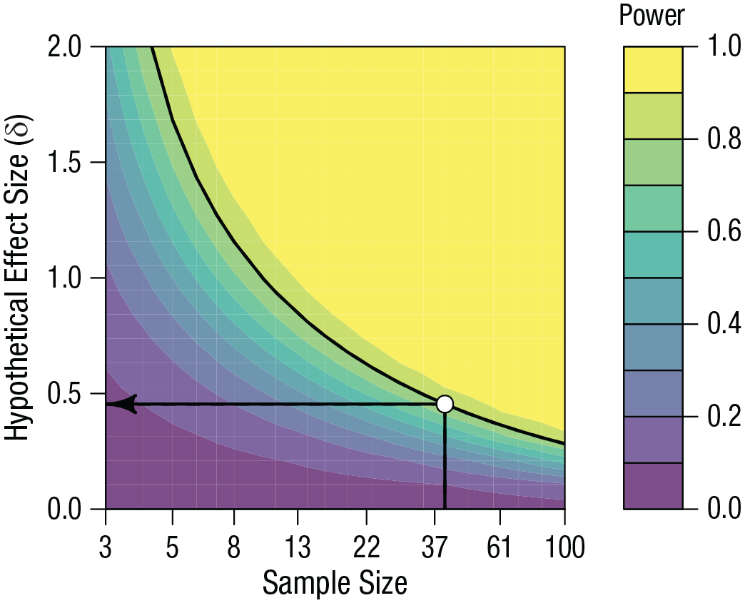
When holding sample size and alpha level constant, the chances of reliably detecting an effect (i.e., power) depends on the hypothetical true effect size. For a within-participants study with 40 participants that uses a paired samples t test to make inferences, there is an 80% chance of detecting an effect size of 0.45. These chances decrease with smaller hypothetical effect sizes. Figure created using the jpower JAMOVI module (https://github.com/richarddmorey/jpower).

In addition to having a lower probability of discovering true effects (Button et al., 2013), study design/test combinations that cannot reliably detect a wide range of effects also have a lower probability that statistically significant results represent true effects (Ioannidis, 2005). In addition, such study design/test combinations tend to be associated with questionable research practices (Dwan et al., 2008) and are more likely to report exaggerated effect sizes (Ioannidis, 2008; Rochefort-Maranda, 2021). In light of these factors, the contribution of low statistical power to the reproducibility crisis in the psychological sciences has become increasingly recognized (Button et al., 2013; Munafò et al., 2017; Walum et al., 2016). However, despite meta-analysis being often considered the “gold standard” of evidence (but see Stegenga, 2011), the role of study-level statistical power for calculating effect sizes in meta-analysis outcomes is rarely considered. This can be a critical oversight because studies included in a meta-analysis that are not designed to reliably detect meaningful effect sizes have reduced evidential value, which diminishes confidence in the body of evidence. Although inverse variance weighting and related approaches can reduce the influence of studies with larger variance (i.e., those with less statistical power) on the summary effect-size estimate, these procedures only attenuate the influence of studies that have larger variances relative to other studies in the meta-analysis. Moreover, this attenuation can be quite modest for random-effects meta-analysis, which is the dominant meta-analysis model in the psychological sciences. Evaluating statistical power for study heterogeneity and moderator tests (Hedges & Pigott, 2004; Huedo-Medina et al., 2006) can also be used to help determine the overall evidential value of a meta-analysis (Bryan et al., 2021; Linden & Hönekopp, 2021); however, these analyses are beyond the scope of this article and associated R package.

One possible reason for the lack of consideration of study-level statistical power in meta-analysis is that it can be time-consuming to calculate statistical power for a body of studies if data were to be directly extracted from each study. A recently proposed solution for calculating study-level statistical power is the sunset (power-enhanced) plot (Fig. 2), which is a feature of the metaviz R package (Kossmeier et al., 2020). Although sunset plots are informative because they visualize the statistical power for all studies included in a meta-analysis, they can visualize statistical power for only one effect size of interest at a time. By default, this effect size is the observed summary effect size calculated for the associated meta-analysis (although statistical power for any single effect size of interest can be calculated).

Fig. 2.

Sunset plots visualize the statistical power for each study included in a meta-analysis for a given hypothetical effect size. The default hypothetical effect size is the observed summary effect size from the associated meta-analysis, but this can be changed to any hypothetical effect size.

Despite the utility of sunset plots, there are some limitations associated with a single effect-size approach. First, unless the meta-analysis comprised only Registered Report studies (Chambers & Tzavella, 2022), it is very likely that the observed summary effect size is inflated because of publication bias (Ioannidis, 2008; Kvarven et al., 2020; Lakens, 2022; Schäfer & Schwarz, 2019). Using Jacob Cohen’s (1988) suggested threshold levels for a small/medium/large effect as an alternative should be avoided as a first option if possible because these thresholds were suggested only as fallback for when the effect-size distribution is unknown. What actually constitutes a small/medium/large effect differs according to subfield (e.g., Gignac & Szodorai, 2016; Quintana, 2016) and study population/context (Kraft, 2020) and is also likely to be influenced by publication bias (Nordahl-Hansen et al., 2022). However, publication bias and issues regarding the inaccuracy of effect-size thresholds are essentially moot points because the true effect size is unknown when testing hypotheses (Lakens, 2022). Alternatively, researchers can determine the range of effect sizes a study design can reliably detect and evaluate whether this range includes meaningful effect sizes. In most cases, determining what constitutes a meaningful effect is not a straightforward task because typical effect sizes vary from field to field and researchers can understandably draw different conclusions. Presenting statistical power assuming a range of true effect sizes, instead of a single true effect size, allows readers to transparently evaluate study-level statistical power according to their own assumptions and what is reasonable for a given research field.

The metameta package has been developed to address these limitations by calculating and visualizing study-level statistical power for a range of hypothetical effect sizes. Along with calculating statistical power for a range of hypothetical effect sizes for each individual study, a median is also calculated across studies to provide an indication of the evidential value of the body of evidence used in a meta-analysis. There are two broad-use cases for the metameta package. The first is the reevaluation of published meta-analysis (e.g., Cherubini & MacDonald, 2021; Quintana, 2020). This could be either for individual meta-analyses or for pooling several meta-analyses on the same topic or in the same research field. Pooling meta-analysis data into a larger analysis is also known as a “meta-meta-analysis” (hence the package name metameta, because this was the original motive for developing the package). The second use case is the implementation of the metameta package when reporting novel meta-analyses (Boen et al., 2022; Gallyer et al., 2021). For example, Gallyer and colleagues (2021) performed a meta-analysis on the link between event-related-potentials derived from electroencephalograms and suicidal thoughts and behaviors and found no significant relationships. An early implementation of the metameta package was used to complement this analysis, which revealed that most included studies were considerably underpowered to detect meaningful effect sizes for the field. Considering this result, the authors concluded that the quality of the evidence was not sufficient to confidently determine the absence of evidence for a relationship. The metameta package is also relevant for helping address Item 15 in the Preferred Reporting Items for Systematic Reviews and Meta-Analyses (PRISMA) 2020 checklist—methods used to assess confidence in the body of evidence (Page et al., 2021)—when reporting meta-analyses.

This purpose of this article is to provide a nontechnical introduction to the metameta package. The R script used in this article and example data sets can be found on OSF at https://osf.io/dr64q/. For readers that are not familiar with R, a companion web app is available at https://dsquintana.shinyapps.io/metameta_app/. The OSF page also contains the R script used to generate the web-browser application for download, which can be used to run the application locally without requiring persistent web access. A screencast video with step-by-step instructions for using the metameta package is also provided at https://bit.ly/3Rol42f and the OSF page.

Package Overview

The metameta package contains three core functions for calculating and visualizing study-level statistical power in meta-analyses for a range of hypothetical effect sizes (Fig. 3). The mapower_se() and mapower_ul() functions perform study-level statistical power calculations, and the firepower() function creates a visualization of these results. The mapower_se() function uses standard-error data, whereas the mapower_ul() function uses 95% confidence interval data to calculate the statistical power associated with a set of studies. The benefit of using standard error and confidence intervals as measures of variance is that at least one of these measures is almost always included in forest-plot visualizations generated by popular meta-analysis software packages. The firepower() function uses output from both these calculator functions (Fig. 3). A ci_to_se() helper function is also included in metameta, which converts 95% confidence intervals to standard errors if the user would prefer to use the mapower_se() function.

Fig. 3.

The metameta package workflow for calculating and visualizing study-level statistical power for a range of hypothetical effect sizes. Data can be imported either with standard errors or confidence intervals as the measure of variance, which determines whether the mapower_se() or mapower_ci() function is used. Both functions will calculate statistical power for a range of hypothetical effect sizes and produce output that can be used for data visualization via the firepower() function.

The metameta package (requiring R Version 3.5 or higher) can be loaded using the following commands, which installs the devtools package, downloads the metameta package from Github, and loads the package:

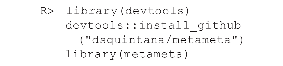
These packages rely on other R packages that may or may not be installed on your system. In some cases, you might be asked if you would like to update existing R packages on your system or if you want to install from sources the package which needs compilation. It has been recommended that you select “no” in response to both these prompts (Harrer et al., 2021), unless an update is required for the package to operate. If you are not familiar or comfortable with R, a point-and-click web-app version of the package is available (https://dsquintana.shinyapps.io/metameta_app/), which is covered in more detail below.

Three meta-analysis data files are also included for demonstration purposes. These meta-analyses synthesize data evaluating the effect of intranasal oxytocin administration on various behavioral and cognitive outcomes; positive values indicate intranasal oxytocin having beneficial effects on outcome measures. Oxytocin is a hormone and neuromodulator produced in the brain, which has been the subject of considerable research in the psychological sciences because of its therapeutic potential for addressing social impairments (Jurek & Neumann, 2018; Leng & Leng, 2021; Quintana & Guastella, 2020). However, this field of research has been associated with mixed results (Alvares et al., 2017), which has partly been attributed to study designs with low statistical power (Quintana, 2020; Walum et al., 2016). The data-set object dat_bakermans_kranenburg contains effect-size and standard-error data from a meta-analysis of 19 studies that investigated the impact of intranasal oxytocin administration on clinical-related outcomes in samples diagnosed with various psychiatric illnesses (Bakermans-Kranenburg & Van Ijzendoorn, 2013). The data-set object dat_keech includes effect-size and confidence-interval data from a meta-analysis on 12 studies that investigated the impact of intranasal oxytocin administration on emotion recognition in neurodevelopmental disorders (Keech et al., 2018). Finally, the data-set object dat_ooi includes effect-size and standard-error data extracted from a meta-analysis of nine studies that investigated the impact of intranasal oxytocin administration on social cognition in autism spectrum disorders (Ooi et al., 2017). These three data sets are also available on OSF at https://osf.io/dr64q/.

Calculating Study-Level Statistical Power for Published Studies

When normally distributed effect sizes (e.g., Hedges g, Cohen’s d, Fisher’s z, log risk-ratio) and their standard errors are available, the statistical power of their study designs for a hypothetical effect size can be calculated using a two-sided Wald test. Some commonly used effect sizes that are not normally distributed include Pearson’s correlation coefficients, risk ratios, and odds ratios. Although the transformation of these effect-size metrics into normally distributed effect sizes is relatively straightforward and typical practice for meta-analysis (Borenstein et al., 2021; Harrer et al., 2021), these untransformed effect-size metrics are sometimes presented in tables or forest plots even if transformed effect sizes are used for meta-analytic synthesis. Thus, metameta users should be wary of this and transform these effect sizes if necessary (Harrer et al., 2021).

The use of the mapower_se() function for calculating study-level statistical power for a range of effect sizes will be illustrated first. The mapower_se() function requires the user to specify a minimum of three arguments: mapower_se(dat, observed_es, name). The first argument (dat) is the data set that contains one column named “yi” (effect-size data) and one column named “sei” (standard-error data). The second argument (observed_es) is the observed summary effect size of the meta-analysis. If effect-size standard errors are not reported, under some circumstances, these can be calculated if sample size information is provided (for a guide on calculating standard errors for both Cohen’s d for between-groups designs and Pearson’s r when sample-size information is available, see Appendix A). Whereas metameta calculates statistical power for a range of hypothetical effect sizes, the statistical power of the observed summary effect size is often of interest for comparison with the full range of effect sizes, so this is presented alongside the statistical power for a range of effect sizes when using the firepower() function, which will be described soon. The third argument (name) is the name of the meta-analysis (e.g., the first author of the meta-analysis), which is used for creating labels when visualizing the data when applying the firepower() function. Data from the dat_ooi data-set object will be used (i.e., Hedges’s g and standard error), which was extracted from Figure 2 from Ooi et al. (2017). Assuming the metameta package is loaded using the command described above (also see the analysis script at https://osf.io/dr64q/), the following R script will calculate study-level statistical power for a range of effect sizes and store this in an object called “power_ooi”:

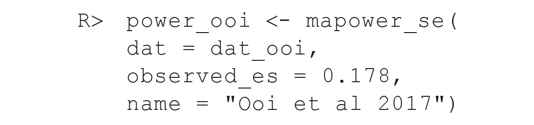
Note that the observed effect size (observed_es) of 0.178 was extracted from forest plot in Figure 2 of Ooi et al. (2017).

The object “power_ooi” contains two data frames. The first data frame, which can be recalled using the power_ooi$dat command, includes the inputted data, statistical power assuming that the observed summary effect size is the true effect size, and statistical power for a range of hypothetical effect sizes, ranging from 0.1 to 1. This range is selected as the default because the majority of reported effect sizes in psychological sciences (Szucs & Ioannidis, 2017) are between 0 and 1, although this range can be adjusted (see below). This information is presented in Table 1 (the last six columns are removed here for the sake of space). These results suggest that none of the included studies could reliably detect effect sizes even as large as 0.4, given that the highest statistical power at this level was 44%. In other words, the study design with highest statistical power (i.e., Study 9) would have only a 44% probability of detecting an effect size of 0.4 (assuming an alpha of .05 and a two-tailed test).

Table 1.

Study-Level Statistical Power for a Range of Effect Sizes and the Observed Effect Size for the Meta-Analysis Reported by Ooi et al. (2016)

Study No.	Study	yi	sei	power_es_observed	power_es01	power_es02	power_es03	power_es04
1	anagnostou_2012	1.19	0.479	0.066	0.055	0.07	0.096	0.133
2	andari_2010	0.155	0.38	0.075	0.058	0.082	0.124	0.183
3	dadds_2014	−0.23	0.319	0.086	0.061	0.096	0.156	0.241
4	domes_2013	−0.185	0.368	0.077	0.059	0.084	0.129	0.192
5	domes_2014	0.824	0.383	0.075	0.058	0.082	0.123	0.181
6	gordon_2013	−0.182	0.336	0.083	0.06	0.091	0.145	0.222
7	guastella_2010	0.235	0.346	0.081	0.06	0.089	0.14	0.212
8	guastella_2015b	0.069	0.279	0.098	0.065	0.111	0.189	0.3
9	watanabe_2014	0.245	0.222	0.126	0.074	0.147	0.272	0.437

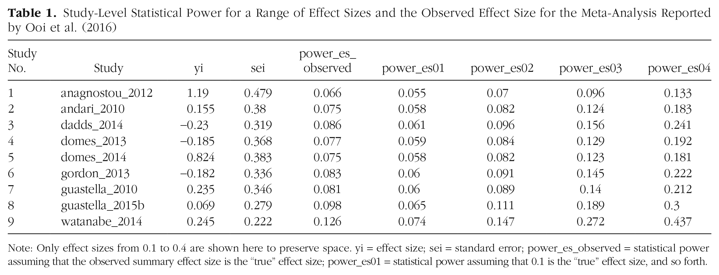
Note: Only effect sizes from 0.1 to 0.4 are shown here to preserve space. yi = effect size; sei = standard error; power_es_observed = statistical power assuming that the observed summary effect size is the “true” effect size; power_es01 = statistical power assuming that 0.1 is the “true” effect size, and so forth.

The second data frame, which can be recalled using the power_ooi$power_median_dat command, includes the median statistical power across all included studies for the observed summary effect size and a range of effect sizes between 0.1 and 1. This output reveals that the median statistical power for all studies assuming a true effect size of 0.4 is 21%. Finally, the firepower() function can be used to create a Firepower plot, which visualizes the median statistical power for a range of effect sizes across all studies included in the meta-analysis. The following command will generate a Firepower plot (Fig. 4) for the Ooi et al. (2017) meta-analysis: firepower(list(power_ooi$power_median_dat)). By default, the firepower() function generates a figure with a generic “Effect size” label on the x-axis. However, it is possible to create a custom label using the (es) argument. For example, here is the same script as above that now includes a “Hedges’ g” label (figure not shown):

Fig. 4.

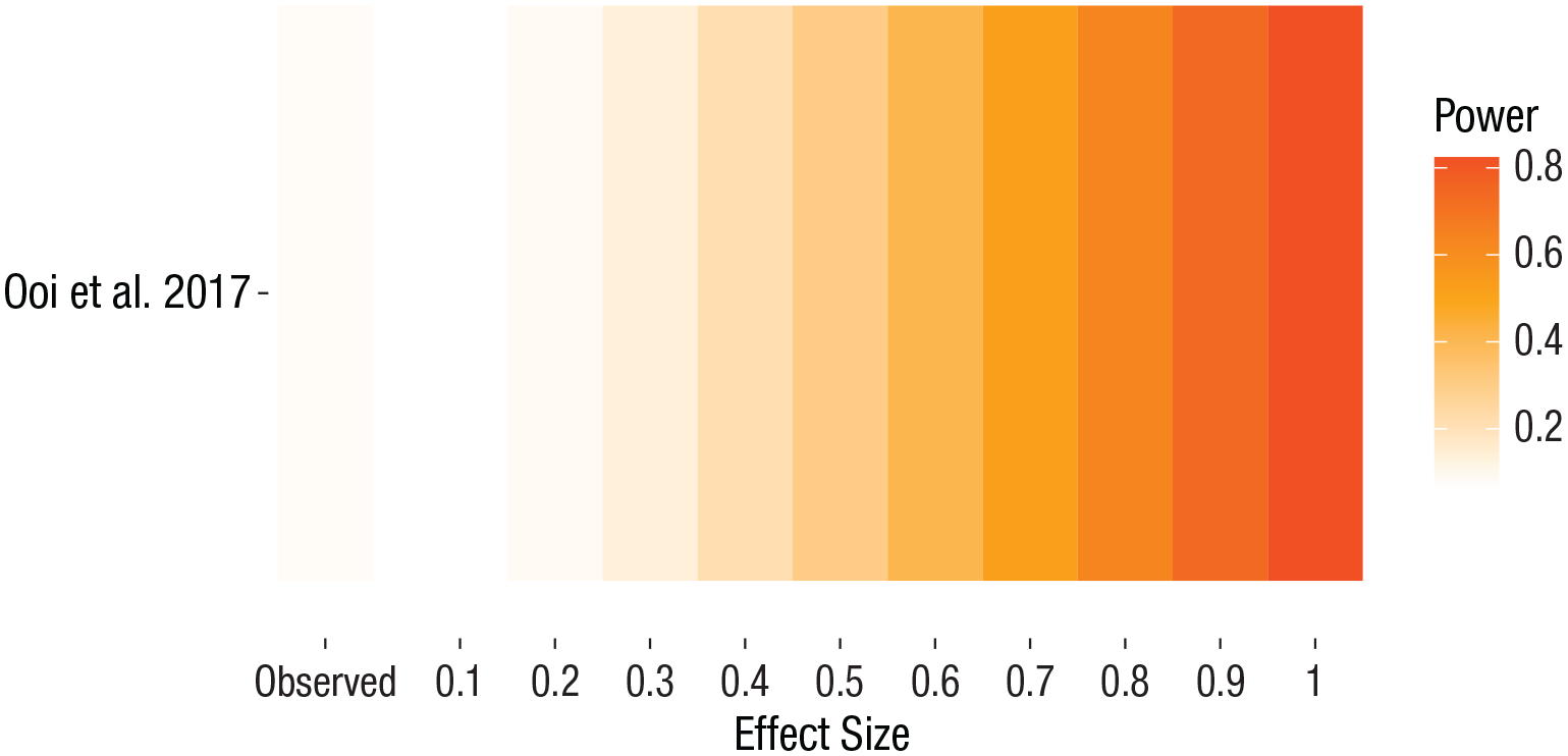
A Firepower plot, which visualizes the median statistical power for a range of hypothetical effect sizes across all studies included in a meta-analysis. The statistical power for the observed summary effect size of the meta-analysis is also shown.

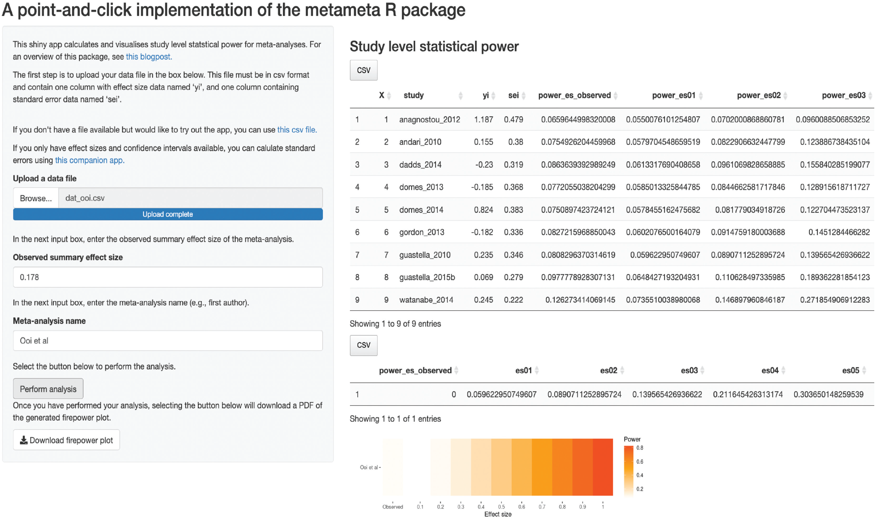
For readers who are not familiar with R, the mapower_se() and firepower() functions have been implemented in a point-and-click web app https://dsquintana.shinyapps.io/metameta_app/ (Fig. 5). To perform the analysis, upload a csv file with effect-size and standard-error data in the format described above, specify the observed effect size, and name the meta-analysis. From the web app, users can download csv files with analysis results and the Firepower plot as a PDF file.

Fig. 5.

A screenshot of the metameta web app. Users can upload csv files with effect sizes and standard-error data, and the app will calculate study-level statistical power for a range of effect sizes, which can be downloaded as a csv file. A Firepower plot, which visualizes statistical power for a range of effect sizes, will also be generated. The Firepower plot can be downloaded as a PDF file. Note that only the first eight columns for study-level statistical power are shown here for the sake of space.

An in-depth interpretation of these results requires an understanding of what constitutes the smallest effect size of interest (SESOI) for the research question at hand. That is, what is the smallest effect size that is considered worthwhile or meaningful? By determining the SESOI, researchers can establish whether a study design/test combination can reliably detect effect sizes that are at least this size or larger. Of course, resource limitations might play a role (e.g., rare populations), so a researcher might have a higher SESOI considering these issues.

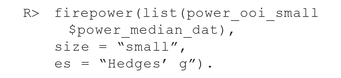
The use of prior effect sizes reported in the literature is one suggestion among others for determining an SESOI (Keefe et al., 2013; Lakens et al., 2018), which will be used an example for how to interpret information provided by the metameta package. For our prior effect size, data from a recent analysis (Quintana, 2020) that indicated that the median effect size across 107 intranasal oxytocin administration trials is 0.14 will be used. This is arguably a conservative estimate because no correction was made for publication-bias inflation in this study. With this value of 0.14 in mind, we return to the results presented in Table 1. Even if we were to round up our SESOI from 0.14 to 0.2, none of these included studies would have more than a 15% chance of detecting this effect size. Moreover, there is an increased chance of a false-positive result for the two statistically significant studies included in this meta-analysis (Ooi et al., 2017), which were Study 1 and Study 9 (Table 1). Altogether, if one were to consider 0.14 as the SESOI of interest, both a significant and nonsignificant meta-analysis result would be largely inconclusive—any nonsignificant results would have an increased chance of being a false negative because these studies were not designed to detect smaller effects, and any significant results are likely to be false positives. For reporting results, one can include the individual study-level data and group-level data with the associated Firepower plot for visualization (Fig. 4). As mentioned above, what constitutes a meaningful or worthwhile effect size (i.e., the SESOI) can differ according to the subfield and a researcher’s interpretation. Although metameta users can provide their own interpretation of the results on the basis of a justified SESOI, a benefit of the output generated by metameta is that it can provide the necessary information for readers to evaluate the credibility of studies or a body of studies according to an SESOI that they have determined.

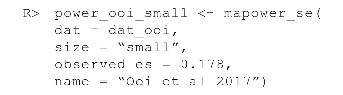
The default setting for the metameta package is for the calculation of power assuming effects that range from 0.1 to 1 in increments of 0.1, which is defined as a “medium” range. Although this range reflects the majority of reported standardized-mean-differences effect sizes in the psychological sciences (Szucs & Ioannidis, 2017), other ranges might be more appropriate for different subfields, disciplines, or effect-size measures (e.g., Pearson’s r). Thus, it is possible to specify a smaller or larger range of effect sizes using an additional optional argument. The “small” option calculates power for a range of effects from 0.05 to 0.5 in increments of 0.05, whereas the “large” option calculates a range of effects from 0.25 to 2.5 in increments of 0.25. For example, the following script will perform the same analysis as above but using instead a smaller range of effect sizes (i.e., 0.05–0.5):

By default, the firepower() function visualizes statistical power for effect sizes ranging from 0.1 to 1, like the mapower_se() function. However, if the “small” or “large” options are used for the “size” argument, then these effect-size ranges can also be visualized via the firepower() function. For example, the “power_ooi_small” object that we just created above can be used to create a Firepower plot, with a “Hedges’ g” label on the x-axis and a “small” effect size range of 0.05 to 0.5 using the following script (figure not shown):

Calculating Power With Effect Sizes and Confidence Intervals

If a meta-analysis does not report standard-error data, it may alternatively present confidence-interval data. The mapower_ul() function facilitates the analysis of effect-size and confidence-interval data using the same four arguments as mapower_se() ; however, the inputted data set requires a different structure. That is, the mapower_ul() function expects a data set containing one column with observed effect sizes or outcomes labeled “yi,” a column labeled “lower” with the lower confidence-interval bound, and column labeled “upper” with the upper confidence-interval bound. This function assumes a 95% confidence interval was used in the meta-analysis the data were extracted from. To demonstrate the mapower_ul() function, data from the dat_keech data-set object will be used (i.e., study name, Hedges’s g, lower confidence interval, and upper confidence interval), which was extracted from Figure 2 from Keech and colleagues (2018).

Assuming the metameta package is loaded, the following R script will calculate study-level statistical power for a range of effect sizes and store this in an object called “power_keech”:

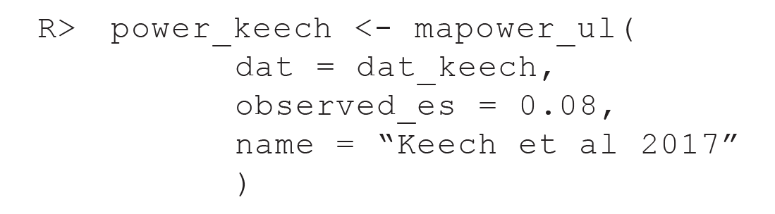
The observed effect size (observed_es) of 0.08 was extracted from forest plot in Figure 2 of Keech et al. (2018). We can recall a data frame containing study-level statistical power for a range of effect sizes using the power_keech$dat command (Table 2), which reveals that at least at the 0.4 effect-size level, two studies were designed to reliably detect effects (using the conventional 80% statistical-power threshold). However, the median statistical power assuming an effect size of 0.4 (calculated extracted using the power_keech$power_median_dat command) was 32%, which is considerably low. As before, we can create a Firepower plot using the following command: firepower(list(power_keech$power_median_dat).

Table 2.

Study-Level Statistical Power for a Range of Effect Sizes and the Observed Effect Size for the Meta-Analysis Reported by Keech et al. (2018)

Study No.	study	yi	lower	upper	sei	power_es_obs	power_es01	power_es02	power_es03	power_es04
1	anagnostou_2012	0.79	−0.12	1.71	0.467	0.053	0.055	0.071	0.098	0.137
2	brambilla_2016	0.15	−0.22	0.52	0.189	0.071	0.083	0.185	0.356	0.563
3	davis_2013	0.11	−0.68	0.9	0.403	0.055	0.057	0.079	0.115	0.168
4	domes_2013	−0.18	−0.86	0.5	0.347	0.056	0.06	0.089	0.139	0.211
5	einfeld_2014	0.22	−0.06	0.51	0.145	0.085	0.106	0.28	0.541	0.786
6	fischer-shofty_2013	0.07	−0.2	0.35	0.14	0.088	0.11	0.297	0.571	0.814
7	gibson_2014	−0.12	−1.13	0.89	0.515	0.053	0.054	0.067	0.09	0.121
8	gordon_2013	−0.15	−0.51	0.2	0.181	0.073	0.086	0.197	0.381	0.598
9	guastella_2010	0.59	0.07	1.12	0.268	0.06	0.066	0.116	0.201	0.321
10	guastella_2015	0.05	−0.54	0.64	0.301	0.058	0.063	0.102	0.169	0.264
11	jarskog_2017	−0.3	−0.83	0.23	0.27	0.06	0.066	0.115	0.199	0.316
12	woolley_2014	−0.01	−0.29	0.26	0.14	0.088	0.11	0.297	0.571	0.814

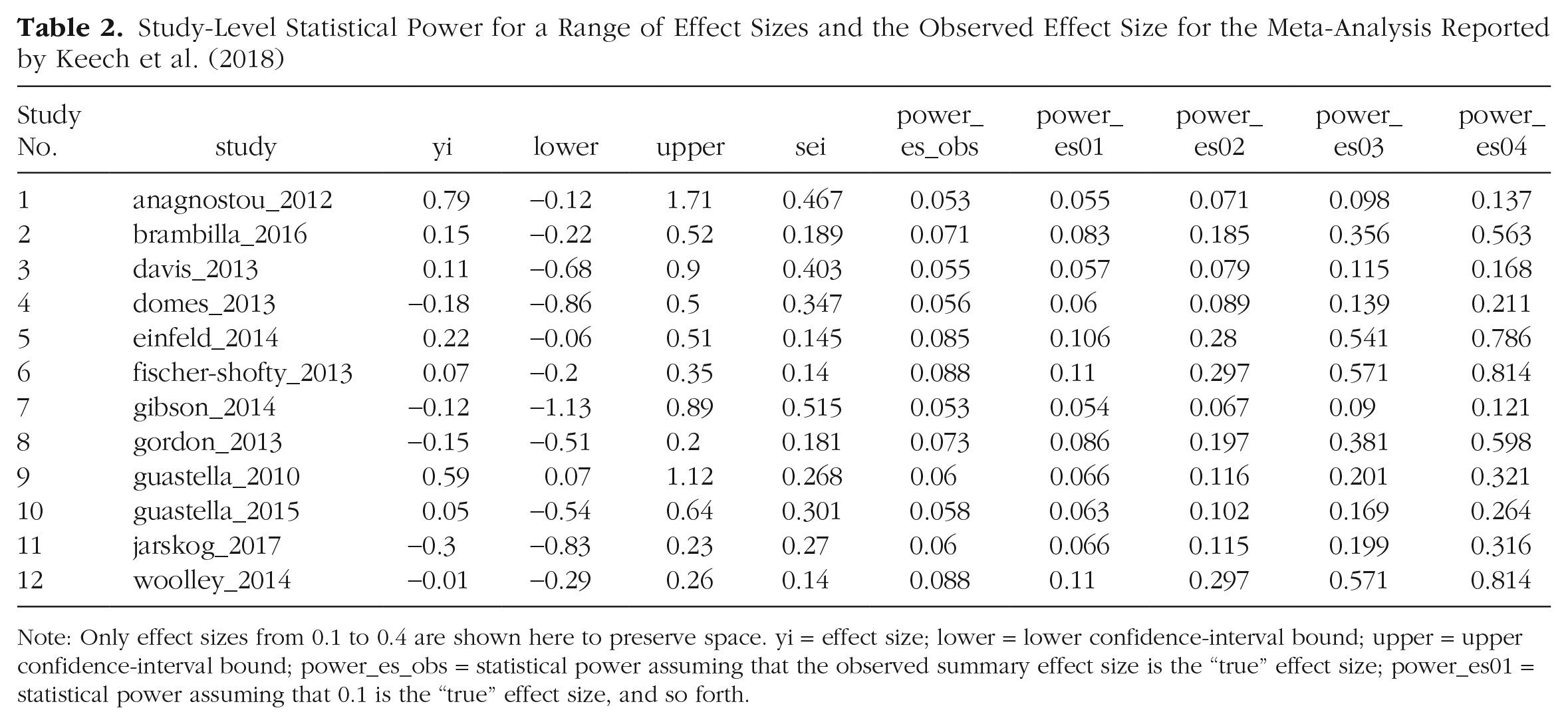
Note: Only effect sizes from 0.1 to 0.4 are shown here to preserve space. yi = effect size; lower = lower confidence-interval bound; upper = upper confidence-interval bound; power_es_obs = statistical power assuming that the observed summary effect size is the “true” effect size; power_es01 = statistical power assuming that 0.1 is the “true” effect size, and so forth.

To use the metameta web-browser application detailed above with confidence-interval data, users first need to convert confidence intervals to standard errors using a companion app, https://dsquintana.shinyapps.io/ci_to_se/. If both standard-error and confidence-interval data are available, these will provide equivalent results, perhaps with some very minor differences because of decimal-place rounding. However, using standard-error data is recommended if both variance data types are available because less data entry is required for the standard-error approach compared with the confidence-interval approach, which reduces the opportunity for data-entry errors. As when using standard-error data, the calculations in the mapower_ul() function assume that effects sizes and their corresponding 95% confidence intervals are normally distributed. Consequently, nonnormally distributed effect sizes (e.g., Pearson’s correlation coefficients, risk ratios, and odds ratios) will need to be transformed into normally distributed effect sizes (Borenstein et al., 2021; Harrer et al., 2021).

Visualizing Study-Level Power Across Multiple Meta-Analyses

Comparing the median study-level statistical power across multiple analyses that use the same effect-size metric is a useful way to evaluate the evidential value of research studies across fields or to compare different subfields. For example, the two previously generated Firepower plots, which both used Hedges’ g as the effect-size metric, can be combined into a single Firepower plot using the following script:

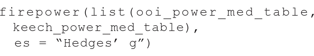
This visualization demonstrates that the studies included in the Keech et al. (2018) meta-analysis were designed to reliably detect a wider range of effect sizes than the studies in the Ooi et al. (2017) meta-analysis (Fig. 6). This approach can also be used when presenting results from multiple novel meta-analyses in the same article, as demonstrated by Boen and colleagues (2022).

Fig. 6.

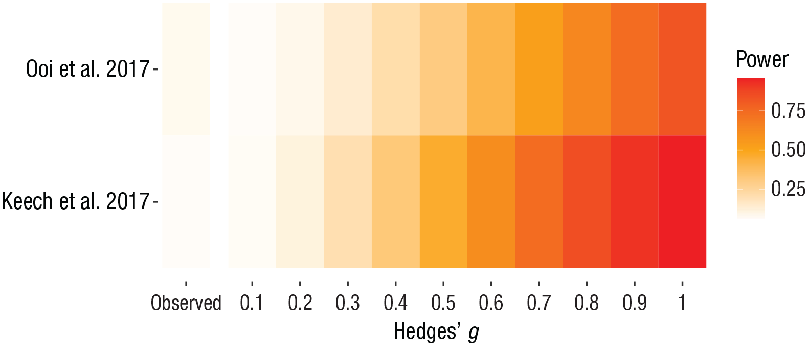
Combining the Firepower plots to facilitate the comparison of study-level statistical power for a range of effect sizes between meta-analyses. This plot reveals that the Keech et al. (2018) meta-analysis contains studies that were designed to reliably detect a wider range of Hedges’s g effect sizes compared with the meta-analysis from Ooi et al. (2017).

Converting Standardized Mean Differences to Biserial Correlation Coefficients to Facilitate Effect-Size Comparison

The previous section presented instructions for comparing study-level power across two or more meta-analyses that use the same effect-size metric. However, in some situations, a meta-analyst may want to synthesize data reported using different effect-size metrics, which can make direct comparison difficult. A plausible scenario for the comparison of two different effect-size metrics is the comparison of studies in which researchers dichotomize one continuous variable into two groups—although this practice in most circumstances has been the subject of critique (MacCallum et al., 2002)—with studies that evaluate the relationship between two continuous variables. In this situation, effect-size conversion is required for comparing study-level statistical power for studies or meta-analyses that use standardized mean differences and correlation coefficients.

A common conversion approach transforms mean differences into a point-biserial correlation coefficient (e.g., Borenstein et al., 2021). However, this method has been shown to demonstrate bias (Jacobs & Viechtbauer, 2017). An alternative method that is largely free of bias is to transform mean-difference data (means, standard deviations, and sample sizes per group) into a biserial correlation coefficient and its variance for comparison with Pearson’s r and its variance (Jacobs & Viechtbauer, 2017). These correlation coefficients can then be reliably combined for meta-analysis and for the calculation of study-level statistical power using the metameta package (Fig. 7). This analysis process is demonstrated in Appendix B.

Fig. 7.

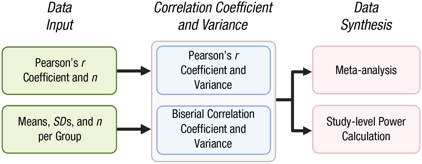
The conversion of standardized mean differences to biserial correlation coefficients can facilitate data synthesis with Pearson’s r coefficients for meta-analysis and the calculation of study-level statistical power.

Calculating Study-Level Statistical Power for New Meta-Analyses

It is relatively straightforward to integrate the calculation of study-level statistical power into the workflow of a novel meta-analysis using the popular metafor package (Viechtbauer, 2010). The escalc() function in metafor calculates effect sizes and their variances from information that is commonly reported (e.g., means).

To use these data in metameta, variance data need to be converted into standard errors by calculating the square root of the effect-size variances. Assuming that your data file is named “dat” and that the variances are in a column named “vi,” you can create a new column with standard errors (sei) using the following script: dat$sei <- sqrt(dat$vi). This updated data set with standard errors can now be used in the mapower_se() function.

Implications for Summary-Effect-Size Statistical Power

One advantage of meta-analysis is that although individual included studies may not have sufficient statistical power to reliably detect a wide range of effect sizes, the synthesis of several of these studies into a summary effect size can increase statistical power. Indeed, a future meta-analysis has been proposed as potential justification for performing studies including small samples because of resource limitations, such as undergraduate student-research projects or when collecting data from rare populations (Lakens, 2022; Quintana, 2021). However, under typical circumstances for the psychological sciences, meta-analysis is not a straightforward remedy for synthesizing underpowered studies, especially those that can reliably detect only large effect sizes because increases in overall power via meta-analysis may be modest.

To illustrate this issue, consider the calculation of statistical power for a meta-analysis set of 10 between-participant experimental studies with an average sample size of 40, low heterogeneity (I² = 25%), and a true effect size of 0.14 (Quintana, 2020), which are parameters analogous to the examples described above. This analysis would suggest that such a research design would have 23% statistical power for a random-effects meta-analysis (Fig. 8a; for R code, see https://osf.io/dr64q/). At least 54 studies would be required to achieve 80% statistical power, holding these other parameters constant. Assuming high heterogeneity (I² = 75%) with these original parameters, statistical power drops to 14% (Fig. 8b), which highlights the impact of study heterogeneity on statistical power. Statistical power for this meta-analysis design with high heterogeneity (I² = 75%) reaches only 80% power with a sample size of 650 (Fig. 7c).

Fig. 8.

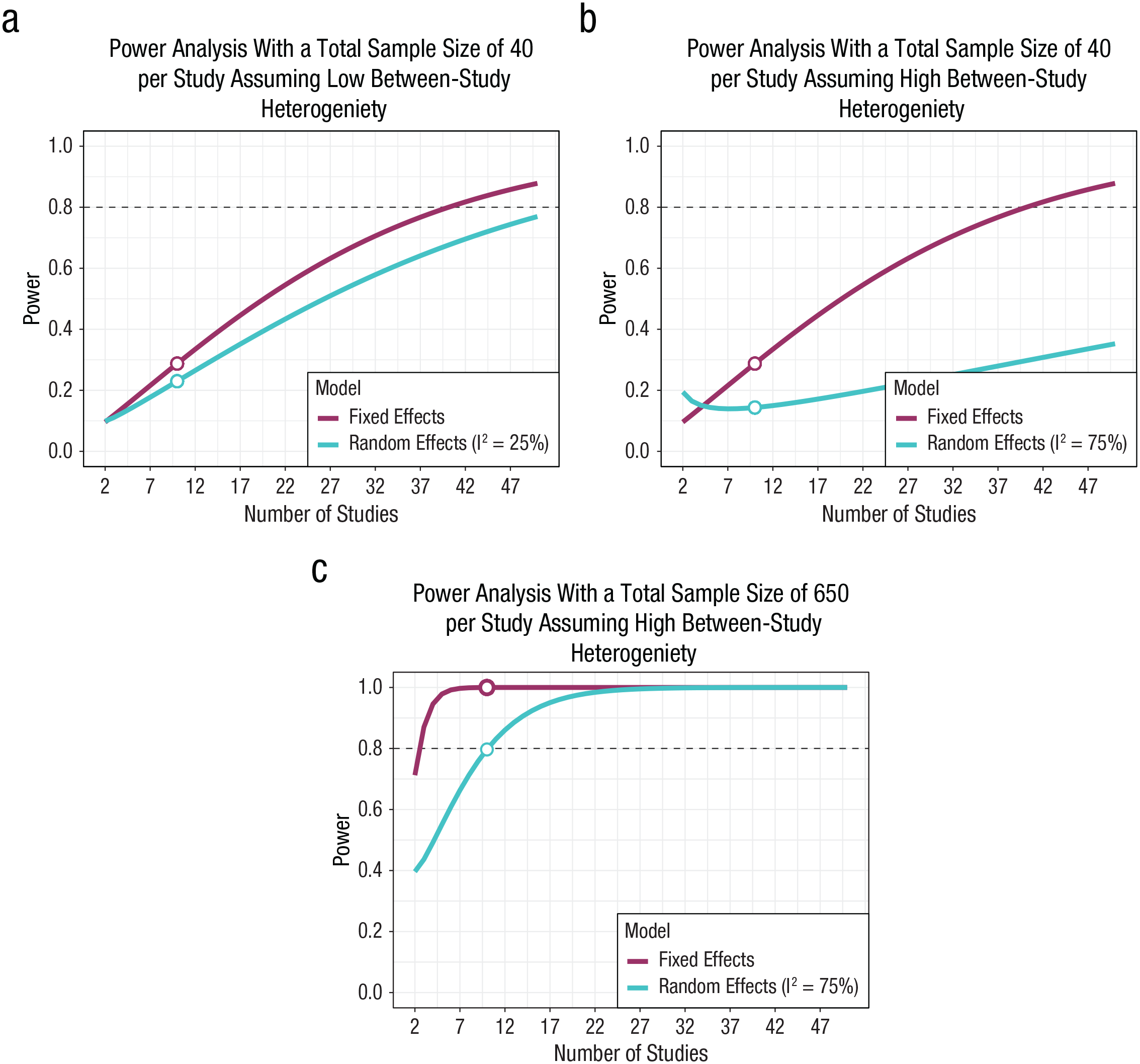
Statistical power analysis for meta-analyses synthesizing between-participants experiments assuming a true effect size of 0.14 for three different scenarios. (a) A random-effects meta-analysis with low heterogeneity (I² = 25%), 10 studies, and 40 participants per study would achieve 24% statistical power. (b) With higher heterogeneity (I² = 75%), statistical power reduces to 14%. (c) Assuming high heterogeneity (I² = 75%), a sample size of 650 is required to achieve statistical power of 80%. The R script to reproduce these figures can be found on OSF at https://osf.io/dr64q/.

Although I just demonstrated that a meta-analysis can theoretically rescue a body of underpowered studies when the effect size of small if there are a large enough number of studies, publication bias (Borenstien et al., 2009) and questionable research practices that tend to be associated with underpowered studies (Dwan et al., 2008) represent formidable problems unless the meta-analysis of small sample sizes and their constituent studies were preplanned and there was a commitment to include study-level data regardless of statistical significance, which is currently rare in practice in the psychological sciences. Preplanning included studies can also reduce between-study heterogeneity because study designs can be better harmonized (Halpern et al., 2002), which would increase meta-analysis statistical power. The Collaborative Replications and Education Project is an example of preplanned meta-analyses of psychology studies that would be statistically underpowered on their own (Wagge et al., 2019). This preplanned meta-analysis approach is more common in medicine (e.g., Simes & The PPP and CTT Investigators, 1995), likely because of the similarity of this approach to multicenter clinical trials. For a retrospective meta-analysis, which is the norm in the psychological sciences, researchers are advised to use methods for the detection of publication bias and potential adjustment of the summary effect size because of publication bias (e.g., Robust Bayesian meta-analysis; Bartoš et al., 2022).

Summary

The metameta package can help evaluate the evidential value of studies included in a meta-analysis by calculating their statistical power. This package extends the existing sunset-plot approach by calculating and visualizing statistical power assuming a range of effect sizes rather than for a single effect size. This tool has been designed to use data that are commonly reported in meta-analysis forest plots—effect sizes and their variances. The increasing recognition of the importance of considering confidence in the body of evidence used in a meta-analysis is reflected in the inclusion of a checklist item on this topic in the recently updated PRISMA checklist (Page et al., 2021). By generating tables and visualizations, the metameta package is well suited to help authors and readers evaluate confidence in a body of evidence.

Statistical power is one of many approaches to evaluate the evidential value of a body of work and should not be used as a stand-alone proxy for study quality or for the overall quality of a meta-analysis. For example, the Grading of Recommendations, Assessment, Development, and Evaluations framework is a common tool for evaluating the quality of evidence in systematic reviews (Balshem et al., 2011), which considers five broad domains: risk of bias (e.g., study design and validity; Flake & Fried, 2020), inconsistency (i.e., heterogeneity; Higgins & Thompson, 2002), indirectness (i.e., the representativeness of study samples; Ghai, 2021; Rad et al., 2018), imprecision (i.e., effect-size variances), and publication bias (van Aert et al., 2019). As demonstrated above (Fig. 8), both inconsistency/heterogeneity and imprecision/variance can have a direct impact on the overall statistical power of a meta-analysis. Of these five domains, publication bias has historically been the most difficult to determine with confidence because researchers need to make decisions about evidence that does not exist, at least publicly (Guyatt et al., 2011). Various tools have more recently been developed for detecting and/or correcting for publication bias, such as robust Bayesian meta-analysis (Bartoš et al., 2022), selection models (Maier et al., 2022; Vevea & Woods, 2005), p-curve (Simonsohn et al., 2014), and z-curve (Brunner & Schimmack, 2020). Another issue that can influence the evidential value of a body of work is the misreporting of statistical test results. Recently developed tools can evaluate the presence of reporting errors, such as GRIM (Brown & Heathers, 2017), SPRITE (Heathers et al., 2018), and statcheck (Nuijten & Polanin, 2020). These misreported statistical-test results are quite common in psychology articles; a 2016 study reported that just under half of a sample of more than 16,000 articles contained at least one statistical inconsistency in which a p value was not consistent with its test statistic and degrees of freedom (Nuijten et al., 2016). This is especially concerning for meta-analyses because test statistics and p values are sometimes used for calculating effect sizes and their variances (Lipsey & Wilson, 2001).

The main purpose of the metameta package is to determine the range of effect sizes that can be reliably detected for a body of studies. This tutorial used an 80% power criterion to determine reliability, but other power levels can be used when justified. Indeed, the 80% power convention does not have a strong empirical basis but, rather, reflected the personal preference of Jacob Cohen (1988; Lakens, 2022). Although a 20% Type II error rate (i.e., 80% statistical power) can be a good starting point judging the evidential value of a study or body of studies, one should consider whether other Type II error rates for the research question at hand are more appropriate (Lakens, 2022; Maier & Lakens, 2022). For example, when working with rare study populations or when collecting observations is expensive, it can be difficult to design studies that can detect small effect sizes given resource limitations because the use of large sample sizes is unrealistic in these cases. Alternatively, in other situations, error rates less than 20% are warranted or more realistic. A benefit of the metameta package is that by presenting power for a range of effects, the readers judge what they consider to be appropriate power given the research question at hand and the available resources.

A key feature of the metameta package is that it is designed to use data that have been extracted from meta-analysis forest plots and tables, which is a much faster process than calculating effect-size and variance data for each individual study. However, this approach assumes that meta-analysis data have been accurately extracted and calculated. For instance, standard errors may have been used instead of standard deviations for meta-analysis calculations, which can influence reported effect sizes and variances (Kadlec et al., 2022). Using the free Zotero reference-manager app (https://www.zotero.org/) can help mitigate this potential error because this app alerts users if they have imported a retracted meta-analysis article or if an article in their database is retracted after being imported. Users should also consider double-checking effect sizes that seem unrealistically large for the research field, which are often due to extraction or calculation errors (Kadlec et al., 2022).

The metameta package has been designed for the straightforward calculation of study-level statistical power and the median statistical power for a body of work when effect-size and variance data are presented in published work or when researchers are reporting new meta-analysis. Conversely, this package is not designed to calculate statistical power for meta-analysis summary effect-size estimates, heterogeneity tests, or moderator tests. However, resources to perform such tests are available elsewhere (Hedges & Pigott, 2004; Huedo-Medina et al., 2006; Valentine et al., 2010). The metameta package is also not designed to work with meta-analyses of nested data (e.g., when several effect sizes are extracted from the same study population) because this would bias the calculations for the median statistical power for a body of research. Another limitation of the package is that it assumes that the range of effect sizes of interest is greater than 0 and less than a value of 2.5, which is the available range for analysis.

The overall goal of this tutorial is to provide an accessible guide for calculating and visualizing the study-level statistical power for meta-analyses for a range of effect sizes using the metameta R package. The companion video tutorial to this article provides additional guidance for readers who are not especially comfortable navigating R scripts. Alternatively, a point-and-click web app has also been provided for people without any programming experience.

Footnotes

Appendix A

Appendix B

Acknowledgements

I am grateful to Pierre-Yves de Müllenheim, who assisted with the web-app script, and to all the people who tested and provided feedback on a beta version of the web app. I am also grateful to Alina Sartorius and Heemin Kang, who tested the R package. Figures 3 and 7 were created using Biorender.com. This manuscript was posted on the OSF preprint server before submission .

Transparency

Action Editor: Pamela Davis-Kean

Editor: David A. Sbarra

Author Contribution(s)

Daniel S. Quintana: Conceptualization; Methodology; Software; Visualization; Writing – original draft.

ORCID iD

Daniel S. Quintana

References

Alexander

R. A.

Scozzaro

M. J.

Borodkin

L. J.

(1989). Statistical and empirical examination of the chi-square test for homogeneity of correlations in meta-analysis. Psychological Bulletin, 106, 329–331. https://doi.org/10.1037/0033-2909.106.2.329

Alvares

G. A.

Quintana

D. S.

Whitehouse

A. J.

(2017). Beyond the hype and hope: Critical considerations for intranasal oxytocin research in autism spectrum disorder. Autism Research, 10(1), 25–41. https://doi.org/10.1002/aur.1692

Bakermans-Kranenburg

M. J.

Van Ijzendoorn

M. H.

(2013). Sniffing around oxytocin: Review and meta-analyses of trials in healthy and clinical groups with implications for pharmacotherapy. Translational Psychiatry, 3, Article e258. https://doi.org/10.1038/tp.2013.34

Balshem

Helfand

Schünemann

H. J.

Oxman

A. D.

Kunz

Brozek

Vist

G. E.

Falck-Ytter

Meerpohl

Norris

Guyatt

G. H.

(2011). GRADE guidelines: 3. Rating the quality of evidence. Journal of Clinical Epidemiology, 64(4), 401–406. https://doi.org/10.1016/j.jclinepi.2010.07.015

Bartoš

Maier

Quintana

D. S.

Wagenmakers

E.-J.

(2022). Adjusting for publication bias in JASP and R: Selection models, PET-PEESE, and robust Bayesian meta-analysis. Advances in Methods and Practices in Psychological Science, 5(3). https://doi.org/10.1177/25152459221109259

Boen

Quintana

D. S.

Ladouceur

C. D.

Tamnes

C. K.

(2022). Age-related differences in the error-related negativity and error positivity in children and adolescents are moderated by sample and methodological characteristics: A meta-analysis. Psychophysiology, 59(6), Article e14003. https://doi.org/10.1111/psyp.14003

Borenstien

Hedges

L. V.

Higgins

J. P. T.

Rothstein

(2009). Introduction to meta-analysis. John Wiley & Sons. https://doi.org/10.1002/9780470743386.ch30

Borenstein

Hedges

L. V.

Higgins

J. P. T.

Rothstein

H. R.

(2021). Introduction to meta-analysis. John Wiley & Sons.

Brown

N. J. L.

Heathers

J. A. J.

(2017). The GRIM test: A simple technique detects numerous anomalies in the reporting of results in psychology. Social Psychological and Personality Science, 8(4), 363–369. https://doi.org/10.1177/1948550616673876

10.

Brunner

Schimmack

(2020). Estimating population mean power under conditions of heterogeneity and selection for significance. Meta-Psychology, 4, Article MP.2018.874. https://doi.org/10.15626/MP.2018.874

11.

Bryan

C. J.

Tipton

Yeager

D. S.

(2021). Behavioural science is unlikely to change the world without a heterogeneity revolution. Nature Human Behaviour, 5(8), 980–989. https://doi.org/10.1038/s41562-021-01143-3

12.

Button

K. S.

Ioannidis

J. P.

Mokrysz

Nosek

B. A.

Flint

Robinson

E. S.

Munafò

M. R.

(2013). Power failure: Why small sample size undermines the reliability of neuroscience. Nature Reviews Neuroscience, 14, 365–376.

13.

Chambers

C. D.

Tzavella

(2022). The past, present and future of Registered Reports. Nature Human Behaviour, 6(1), 29–42. https://doi.org/10.1038/s41562-021-01193-7

14.

Cherubini

J. M.

MacDonald

M. J.

(2021). Statistical inferences using effect sizes in human endothelial function research. Artery Research, 27(4), 176–185. https://doi.org/10.1007/s44200-021-00006-6

15.

Cohen

(1988). Statistical power analysis for the behavioural sciences. Erlbaum.

16.

Dwan

Altman

D. G.

Arnaiz

J. A.

Bloom

Chan

A.-W.

Cronin

Decullier

Easterbrook

P. J.

Elm

E. V.

Gamble

Ghersi

Ioannidis

J. P.

Simes

Williamson

P. R.

(2008). Systematic review of the empirical evidence of study publication bias and outcome reporting bias. PLOS ONE, 3(8), Article e3081. https://doi.org/10.1371/journal.pone.0003081

17.

Flake

J. K.

Fried

E. I.

(2020). Measurement schmeasurement: Questionable measurement practices and how to avoid them. Advances in Methods and Practices in Psychological Science, 3(4), 456–465. https://doi.org/10.1177/2515245920952393

18.

Gallyer

A. J.

Dougherty

S. P.

Burani

Albanese

B. J.

Joiner

T. E.

Hajcak

(2021). Suicidal thoughts, behaviors, and event-related potentials: A systematic review and meta-analysis. Psychophysiology, 58(12), Article e13939. https://doi.org/10.1111/psyp.13939

19.

Ghai

(2021). It’s time to reimagine sample diversity and retire the WEIRD dichotomy. Nature Human Behaviour, 5(8), Article 8. https://doi.org/10.1038/s41562-021-01175-9

20.

Gignac

G. E.

Szodorai

E. T.

(2016). Effect size guidelines for individual differences researchers. Personality and Individual Differences, 102, 74–78. https://doi.org/10.1016/j.paid.2016.06.069

21.

Guyatt

G. H.

Oxman

A. D.

Montori

Vist

Kunz

Brozek

Alonso-Coello

Djulbegovic

Atkins

Falck-Ytter

Williams

J. W.

Meerpohl

Norris

S. L.

Akl

E. A.

Schünemann

H. J.

(2011). GRADE guidelines: 5. Rating the quality of evidence—Publication bias. Journal of Clinical Epidemiology, 64(12), 1277–1282. https://doi.org/10.1016/j.jclinepi.2011.01.011

22.

Halpern

S. D.

Karlawish

J. H. T.

Berlin

J. A.

(2002). The continuing unethical conduct of underpowered clinical trials. Journal of the American Medical Association, 288(3), 358–362. https://doi.org/10.1001/jama.288.3.358

23.

Harrer

Cuijpers

Furukawa

T. A.

Ebert

D. D.

(2021). Doing meta-analysis in R: A hands-on guide. Chapman & Hall/CRC Press. https://bookdown.org/MathiasHarrer/Doing_Meta_Analysis_in_R/

24.

Heathers

J. A.

Anaya

van der Zee

Brown

N. J.

(2018). Recovering data from summary statistics: Sample Parameter Reconstruction via Iterative TEchniques (SPRITE). PeerJ Preprints, 6, Article e26968v1. https://doi.org/10.7287/peerj.preprints.26968v1

25.

Hedges

L. V.

Pigott

T. D.

(2004). The power of statistical tests for moderators in meta-analysis. Psychological Methods, 9(4), 426–445. https://doi.org/10.1037/1082-989X.9.4.426

26.

Higgins

J. P. T.

Thompson

S. G.

(2002). Quantifying heterogeneity in a meta-analysis. Statistics in Medicine, 21(11), 1539–1558. https://doi.org/10.1002/sim.1186

27.

Huedo-Medina

T. B.

Sánchez-Meca

Marín-Martínez

Botella

(2006). Assessing heterogeneity in meta-analysis: Q statistic or I2 index? Psychological Methods, 11(2), 193–206. https://doi.org/10.1037/1082-989X.11.2.193

28.

Ioannidis

J. P.

(2005). Why most published research findings are false. PLOS Medicine, 2(8), Article e124. https://doi.org/10.1371/journal.pmed.0020124

29.

Ioannidis

J. P.

(2008). Why most discovered true associations are inflated. Epidemiology, 19, 640–648. https://doi.org/10.1097/EDE.0b013e31818131e7

30.

Jacobs

Viechtbauer

(2017). Estimation of the biserial correlation and its sampling variance for use in meta-analysis. Research Synthesis Methods, 8(2), 161–180. https://doi.org/10.1002/jrsm.1218

31.

Jurek

Neumann

I. D.

(2018). The oxytocin receptor: From intracellular signaling to behavior. Physiological Reviews, 98(3), 1805–1908. https://doi.org/10.1152/physrev.00031.2017

32.

Kadlec

Sainani

K. L.

Nimphius

(2022). With great power comes great responsibility: Common errors in meta-analyses and meta-regressions in strength & conditioning research. Sports Medicine. Advance online publication. https://doi.org/10.1007/s40279-022-01766-0

33.

Keech

Crowe

Hocking

D. R.

(2018). Intranasal oxytocin, social cognition and neurodevelopmental disorders: A meta-analysis. Psychoneuroendocrinology, 87, 9–19. https://doi.org/10.1016/j.psyneuen.2017.09.022

34.

Keefe

R. S. E.

Kraemer

H. C.

Epstein

R. S.

Frank

Haynes

Laughren

T. P.

McNulty

Reed

S. D.

Sanchez

Leon

A. C.

(2013). Defining a clinically meaningful effect for the design and interpretation of randomized controlled trials. Innovations in Clinical Neuroscience, 10(5–6, Suppl. A), 4S–19S.

35.

Kossmeier

Tran

U. S.

Voracek

(2020). Power-enhanced funnel plots for meta-analysis: The sunset funnel plot. Zeitschrift Für Psychologie, 228(1), 43–49. https://doi.org/10.1027/2151-2604/a000392

36.

Kraft

M. A.

(2020). Interpreting effect sizes of education interventions. Educational Researcher, 49(4), 241–253. https://doi.org/10.3102/0013189X20912798

37.

Kvarven

Strømland

Johannesson

(2020). Comparing meta-analyses and preregistered multiple-laboratory replication projects. Nature Human Behaviour, 4(4), 423–434. https://doi.org/10.1038/s41562-019-0787-z

38.

Lakens

(2022). Sample size justification. Collabra: Psychology, 8(1), Article 33267. https://doi.org/10.1525/collabra.33267

39.

Lakens

Scheel

A. M.

Isager

P. M.

(2018). Equivalence testing for psychological research: A tutorial. Advances in Methods and Practices in Psychological Science, 1(2), 259–269. https://doi.org/10.1177/2515245918770963

40.

Leng

R. I.

(2021). Oxytocin: A citation network analysis of 10 000 papers. Journal of Neuroendocrinology, 33, Article e13014. https://doi.org/10.1111/jne.13014

41.

Linden

A. H.

Hönekopp

(2021). Heterogeneity of research results: A new perspective from which to assess and promote progress in psychological science. Perspectives on Psychological Science, 16(2), 358–376. https://doi.org/10.1177/1745691620964193

42.

Lipsey

M. W.

Wilson

D. B.

(2001). Practical meta-analysis. Sage.

43.

MacCallum

R. C.

Zhang

Preacher

K. J.

Rucker

D. D.

(2002). On the practice of dichotomization of quantitative variables. Psychological Methods, 7, 19–40. https://doi.org/10.1037/1082-989X.7.1.19

44.

Maier

Lakens

(2022). Justify your alpha: A primer on two practical approaches. Advances in Methods and Practices in Psychological Science, 5(2). https://doi.org/10.1177/25152459221080396

45.

Maier

VanderWeele

T. J.

Mathur

M. B.

(2022). Using selection models to assess sensitivity to publication bias: A tutorial and call for more routine use. Campbell Systematic Reviews, 18(3), Article e1256. https://doi.org/10.1002/cl2.1256

46.

Munafò

M. R.

Nosek

B. A.

Bishop

D. V.

Button

K. S.

Chambers

C. D.

Du Sert

N. P.

Simonsohn

Wagenmakers

E.-J.

Ware

J. J.

Ioannidis

J. P.

(2017). A manifesto for reproducible science. Nature Human Behaviour, 1(1), Article 0021. https://doi.org/10.1038/s41562-016-0021

47.

Nordahl-Hansen

Cogo-Moreira

Panjeh

Quintana

(2022). Redefining effect size interpretations for psychotherapy RCTs in depression. OSF Preprints. https://doi.org/10.31219/osf.io/erhmw

48.

Nuijten

M. B.

Hartgerink

C. H. J.

van Assen

M. A. L. M.

Epskamp

Wicherts

J. M.

(2016). The prevalence of statistical reporting errors in psychology (1985–2013). Behavior Research Methods, 48(4), 1205–1226. https://doi.org/10.3758/s13428-015-0664-2

49.

Nuijten

M. B.

Polanin

J. R.

(2020). “statcheck”: Automatically detect statistical reporting inconsistencies to increase reproducibility of meta-analyses. Research Synthesis Methods, 11(5), 574–579. https://doi.org/10.1002/jrsm.1408

50.

Page

M. J.

McKenzie

J. E.

Bossuyt

P. M.

Boutron

Hoffmann

T. C.

Mulrow

C. D.

Shamseer

Tetzlaff

J. M.

Akl

E. A.

Brennan

S. E.

Chou

Glanville

Grimshaw

J. M.

Hróbjartsson

Lalu

M. M.

Loder

E. W.

Mayo-Wilson

McDonald

. . . Moher

(2021). The PRISMA 2020 statement: An updated guideline for reporting systematic reviews. The BMJ, 372, Article n71. https://doi.org/10.1136/bmj.n71

51.

Quintana

D. S.

(2015). From pre-registration to publication: A nontechnical primer for conducting a meta-analysis to synthesize correlational data. Frontiers in Psychology, 6, Article 1549. https://doi.org/10.3389/fpsyg.2015.01549

52.

Quintana

D. S.

(2016). Statistical considerations for reporting and planning heart rate variability case-control studies. Psychophysiology, 54(3), 344–349. https://doi.org/10.1111/psyp.12798

53.

Quintana

D. S.

(2020). Most oxytocin administration studies are statistically underpowered to reliably detect (or reject) a wide range of effect sizes. Comprehensive Psychoneuroendocrinology, 4, Article 100014. https://doi.org/10.1016/j.cpnec.2020.100014

54.

Quintana

D. S.

(2021). Replication studies for undergraduate theses to improve science and education. Nature Human Behaviour, 5(9), 1117–1118. https://doi.org/10.1038/s41562-021-01192-8

55.

Quintana

D. S.

Guastella

A. J.

(2020). An allostatic theory of oxytocin. Trends in Cognitive Sciences, 24(7), 515–528. https://doi.org/10.1016/j.tics.2020.03.008

56.

Rad

M. S.

Martingano

A. J.

Ginges

(2018). Toward a psychology of Homo sapiens: Making psychological science more representative of the human population. Proceedings of the National Academy of Sciences, USA, 115(45), 11401–11405. https://doi.org/10.1073/pnas.1721165115

57.

Rochefort-Maranda

(2021). Inflated effect sizes and underpowered tests: How the severity measure of evidence is affected by the winner’s curse. Philosophical Studies, 178(1), 133–145. https://doi.org/10.1007/s11098-020-01424-z

58.

Schäfer

Schwarz

M. A.

(2019). The meaningfulness of effect sizes in psychological research: Differences between sub-disciplines and the impact of potential biases. Frontiers in Psychology, 10, Article 813. https://doi.org/10.3389/fpsyg.2019.00813

59.

Simes

R. J.

, & The PPP and CTT Investigators. (1995). Prospective meta-analysis of cholesterol-lowering studies: The prospective pravastatin pooling (PPP) project and the cholesterol treatment trialists (CTT) collaboration. The American Journal of Cardiology, 76(9, Suppl. 1), 122C–126C. https://doi.org/10.1016/S0002-9149(99)80482-2

60.

Simonsohn

Nelson

L. D.

Simmons

J. P.

(2014). p-curve and effect size: Correcting for publication bias using only significant results. Perspectives on Psychological Science, 9(6), 666–681. https://doi.org/10.1177/1745691614553988

61.

Stegenga

(2011). Is meta-analysis the platinum standard of evidence? Studies in History and Philosophy of Science Part C: Biological and Biomedical Sciences, 42(4), 497–507. https://doi.org/10.1016/j.shpsc.2011.07.003

62.

Szucs

Ioannidis

J. P.

(2017). Empirical assessment of published effect sizes and power in the recent cognitive neuroscience and psychology literature. PLOS Biology, 15(3), Article e2000797. https://doi.org/10.1371/journal.pbio.2000797

63.

Valentine

J. C.

Pigott

T. D.

Rothstein

H. R.

(2010). How many studies do you need?: A primer on statistical power for meta-analysis. Journal of Educational and Behavioral Statistics, 35(2), 215–247. https://doi.org/10.3102/1076998609346961

64.

van Aert

R. C. M.

Wicherts

J. M.

van Assen

M. A. L. M

. (2019). Publication bias examined in meta-analyses from psychology and medicine: A meta-meta-analysis. PLOS ONE, 14(4), Article e0215052. https://doi.org/10.1371/journal.pone.0215052

65.

Vevea

Woods

(2005). Publication bias in research synthesis: Sensitivity analysis using a priori weight functions. Psychological Methods, 10(4), 428–443. https://doi.org/10/dtwt9h

66.

Viechtbauer

(2010). Conducting meta-analyses in R with the metafor package. Journal of Statistical Software, 36, 1–48. https://doi.org/10.18637/jss.v036.i03

67.

Wagge

J. R.

Brandt

M. J.

Lazarevic

L. B.

Legate

Christopherson

Wiggins

Grahe

J. E.

(2019). Publishing research with undergraduate students via replication work: The Collaborative Replications and Education Project. Frontiers in Psychology, 10, Article 247. https://doi.org/10.3389/fpsyg.2019.00247

68.

Walum

Waldman

I. D.

Young

L. J.

(2016). Statistical and methodological considerations for the interpretation of intranasal oxytocin studies. Biological Psychiatry, 79, 251–257. https://doi.org/10.1016/j.biopsych.2015.06.016