
Abstract
Researchers across many fields have called for greater attention to heterogeneity of treatment effects—shifting focus from the average effect to variation in effects between different treatments, studies, or subgroups. True heterogeneity is important, but many reports of heterogeneity have proved to be false, nonreplicable, or overestimated. In this review, we catalog ways that past researchers fooled themselves about heterogeneity and recommend ways that we, as researchers, can stop fooling ourselves about heterogeneity in the future. We make 18 specific recommendations. The most common themes are to (a) seek heterogeneity only when the mechanism offers clear motivation and the data offer adequate power, (b) shy away from seeking “no-but” heterogeneity when there is no main effect, (c) separate the noise of estimation error from the signal of true heterogeneity, (d) shrink variation in estimates toward zero, (e) increase p values and widen confidence intervals when conducting multiple tests, (f) estimate interactions rather than subgroup effects, and (g) check whether findings of heterogeneity are sensitive to changes in model or measurement. We also resolve long-standing debates about centering interactions in linear models and estimating interactions in nonlinear models, such as logistic, ordinal, and interval regression. If researchers follow these recommendations, the search for heterogeneity should yield more trustworthy results in the future.
In recent years, many scholars have called attention to heterogeneity—the idea that treatment effects vary across individuals, populations, contexts, and studies. Although most research still focuses on estimating main effects, or how well treatments work on average, research on heterogeneity asks when, where, and for whom treatment works best or worst.
Enthusiasm for heterogeneity spans many disciplines (e.g., Bolger et al., 2019; McShane et al., 2019; Schudde, 2018). Leading researchers in statistics and social psychology have criticized a focus on main effects as “parochial” and stated that “behavioral science is unlikely to change the world without a heterogeneity revolution” (Bryan et al., 2021, p. 980). Conferences and thematic issues have urged contributors to look for heterogeneity in education, sociology, economics, psychopathology, and policy research (e.g., Torche et al., 2024; Damme & Mittal, 2023; Reardon & Stuart, 2017). Some medical researchers hope that a better understanding of heterogeneity will usher in an age of “personalized” or “precision medicine” in which patients receive treatment tailored to their specific needs instead of an off-the-rack treatment that works only on average (Kosorok & Laber, 2019). Likewise, some psychotherapy scholars have outlined a vision for a “personalized science of human improvement” (Hayes et al., 2022) that tailors psychotherapy to an individual’s personality, behaviors, goals, and needs.
The importance of true heterogeneity is undeniable. One need look no further than the recent COVID-19 pandemic for examples. Infection with the COVID-19 virus was most dangerous for adults who were older or suffered from certain preexisting conditions. Knowing which groups were most vulnerable was vital for prioritizing access to vaccines when they first became available in limited supply (Persad et al., 2020). Some vaccines proved to be more effective than others (Self, 2021), and knowing that influenced patients and providers in deciding when to pursue an opportunity for vaccination and when to pass. Remote schooling during the pandemic depressed achievement most for children in high-poverty schools, and that was an important consideration when prioritizing federal aid intended to facilitate academic recovery (Goldhaber et al., 2022).
Yet for 7 decades, efforts to identify heterogeneity have yielded disappointing results. In a 1957 presidential address to the American Psychological Association (APA), Lee Cronbach called for a kind of heterogeneity revolution. “Assigning everyone to the treatment with the highest average [response] is rarely the best decision,” he wrote. “Ultimately, we should design treatments not to fit the average person, but to fit groups of students with particular aptitude patterns” (Cronbach, 1957, pp. 680–682). Cronbach charged psychologists to go forth and find “aptitude-treatment interactions,” where aptitude was defined to include “innate differences, motivation, and past experience”—in short, as he later clarified, “any characteristic of the person that affects his response to the treatment” (Cronbach, 1975, p. 116).
By 1975, though, in another APA address, Cronbach reported that the search for “interactions did not turn out as we had anticipated” (Cronbach, 1975, p. 119). Few theorized interactions had materialized, and those that had materialized had triggered a replication crisis (Hedges & Schauer, 2018). “I have been thwarted by the inconsistent findings coming from roughly similar inquiries,” Cronbach wrote. “Successive studies employing the same treatment variable find different interactions” (Cronbach, 1975, p. 119). Cronbach conjectured that limiting inquiry to two-way interactions had been naive and that three-way, four-way, and higher-order interactions might be needed to clarify the circumstances and populations in which an intervention was or was not effective. Given the number of higher-order interactions that were possible and the small sample sizes then available to test them, it seemed “unlikely that social scientists will be able to establish [reliable] generalizations” about moderated effects (Cronbach, 1975, p. 116). The search for heterogeneity had led into a “hall of mirrors that extends to infinity” (Cronbach, 1975, p. 119).
From the 1970s to the early 1990s, “many authors . . . lamented the difficulty of detecting reliable moderator effects” and grew “so frustrated by not finding theorized moderator effects that they continue[d] to use and to invent inappropriate statistical procedures” that produced spurious findings of heterogeneity (McClelland & Judd, 1993, p. 377). Truly heterogeneous effects were described in the psychotherapy literature as “infrequent, undependable, and difficult to detect” (Smith & Sechrest, 1991, p. 233).
Even in recent years, as enthusiasm for heterogeneity has revived, some researchers have maintained a skeptical attitude. In organization research, a 2017 review article concluded that “the empirical track record of moderator variable studies is very discouraging,” suggesting that scholars need to “mend it or end it” when it comes to searching for heterogeneity (Murphy & Russell, 2017, p. 549). Even when significant, most interactions in psychology are disappointingly small; on a standardized scale, the median interaction is only .05, meaning that the moderator usually changes the treatment effect by .05 SD or less (Aguinis et al., 2005; Baranger et al., 2022). In medicine, some reporters and scholars believe enthusiasm for precision medicine is premature given that fewer than 7% of cancer patients, for example, have the potential to benefit from available drugs tailored to their personal genome (Marquart et al., 2018; Prasad, 2016; Szabo, 2018). Shares of the consumer genomics company 23AndMe have fallen from more than $300 to less than $3 after the company failed to provide value in the form of “personalized wellness plans” tailored to subscribers’ genetic profile (Winkler, 2024).
The resurgence of interest in heterogeneity stems in part from concerns about the replication crisis. A substantial fraction of main effects fail to replicate when tested in new contexts and populations (Boulay et al., 2018; Ioannidis, 2005; Open Science Collaboration, 2015). Some failures to replicate main effects may result from inattention to hidden moderators, which might explain why a treatment worked in one setting but not in another (Bryan et al., 2021, p. 981). For example, some social-psychology findings replicate better among college students, where they were discovered, than in broader populations (Yeager et al., 2019), suggesting that effects are moderated by participants’ age and education. Likewise, the facial-feedback effect—the hypothesis that smiling, for example, makes the smiler happier—may replicate only when the experimenter is present to see the smiler’s face and not when the experimenter is absent (Phaf & Rotteveel, 2024). Despite these encouraging examples, a review of 68 meta-analyses of replication studies in psychology found limited evidence of heterogeneity across time, situations, and persons, leading the authors to describe their findings as “an argument against so-called ‘hidden moderators’” (Olsson-Collentine et al., 2020, p. 936).
In fact, despite the hope that moderators might solve the replication crisis, moderated effects have proved to be less replicable than main effects. Across four large-scale efforts to replicate published results in psychology, economics, and social science, only one in five moderated effects (interactions) replicated successfully, versus half of main effects (Altmejd et al., 2019; Open Science Collaboration, 2015). In a review of clinical trials, out of 117 subgroup effects claimed in study abstracts, only five had been subjected to replication attempts, and none of those attempts successfully replicated the subgroup effect (Wallach et al., 2017). In short, although attention to heterogeneity may sometimes clear up the mystery of a nonreplicable effect, to date, it seems that the pursuit of moderators—at least as it has typically been conducted—may have made the replication crisis worse instead of better.
None of this means that heterogeneity is nonexistent or impossible to detect. But it does suggest that modern researchers should be more careful than their predecessors when looking for heterogeneous effects.
In this article, we diagnose major reasons for past disappointments and make 18 concrete recommendations that should reduce disappointments in the future. We explain how so many past scholars have fooled themselves about heterogeneity and recommend steps to ensure that “we don’t get fooled again” (Townshend, 1971).
Overview
Our plan for the article is as follows. We start by clarifying terminology in a section titled “What We Talk About When We Talk About Heterogeneity.” Among other things, our terminology highlights the key distinction between heterogeneity that one can explain through treatment-moderator interactions and heterogeneity that remains unexplained and simply represents variation in effects from one study, treatment, time, or place to another.
We then group 18 recommendations into three broad sections: “How Not to Fool Ourselves About Unexplained Heterogeneity,” “How Not to Fool Ourselves About Explained Heterogeneity,” and “How Not to Let Models and Measures Fool Us About Heterogeneity.” Our discussion of heterogeneity is not exhaustive, but we spotlight the most common pitfalls encountered in the search for heterogeneity, and we recommend ways to avoid them.
What We Talk About When We Talk About Heterogeneity
Before we get started, we explain what we mean by “heterogeneity” because the word means different things in different settings.
Explained versus unexplained heterogeneity
The most important distinction for our purposes is the distinction between explained and unexplained heterogeneity. These terms are meant to evoke the distinction between explained and unexplained variance in regression, where explained variance is associated with specific explanatory variables and unexplained variance is not.
Explained heterogeneity
Many experimental and observational studies try to explain why effects vary by identifying specific moderator variables that predict larger or smaller effects. We call this “explained heterogeneity”; it is also called “moderation.” Attempts to explain heterogeneity often estimate interactions between the treatment and one or more moderator variables.
We explained heterogeneity in our introduction when we observed that the first COVID-19 vaccines had larger benefits for the elderly and that pandemic school closures did greater harm to children from low-income families. In other words, age explained or moderated the effects of the vaccine, and income explained or moderated the effects of school closures.
Unexplained heterogeneity
Other studies estimate how much effects vary without trying to associate that variation with moderator variables. We call this “unexplained heterogeneity.”
One research design that highlights unexplained heterogeneity is meta-analysis, which combines the results of several studies to estimate an average treatment effect and the variance across studies that is due to heterogeneity—which in a simple meta-analysis means unexplained heterogeneity. In a more complex meta-analysis, researchers may try to explain heterogeneity by comparing studies with different characteristics. Moderator or subgroup analysis estimates the relationship between effect size and a single study characteristic, whereas metaregression can model the relationship between effect sizes and multiple study characteristics simultaneously (Viswesvaran & Sanchez, 1998).
Another design that highlights unexplained heterogeneity is a megastudy, which assigns many different treatments, ideally at random, to different participants in a study population (Milkman, Gromet, et al., 2021). The goal of a megastudy is typically to identify and select the most effective treatments without necessarily trying to explain why some treatments were more effective than others. For example, one megastudy tried to identify which of many text messages did the most to increase participants’ vaccination rates (Milkman, Patel, et al., 2021), and another tried to identify which of many hints did the most to help students to solve math problems (Haim et al., 2022).
A popular type of megastudy is a value-added study, which highlights unexplained heterogeneity among teachers—trying to identify which of many teachers had the largest effects on student test scores without necessarily trying to explain why. Because students are not assigned to teachers at random, value-added studies commonly control for prior test scores and other covariates (Staiger & Rockoff, 2010).
The bulk of heterogeneity is often unexplained
In many studies, the bulk of heterogeneity remains unexplained. After every available moderator has been considered, it often remains largely unclear why effects vary from one study, setting, or individual to another. For example, although age explained some heterogeneity in the benefits of the COVID vaccines, there were elderly individuals who died despite being vaccinated or experienced minimal symptoms despite being unvaccinated. Likewise, although family income explained some of the heterogeneity in the learning effects of pandemic school closures, there were many high-income families whose children learned little during the pandemic. And although teachers clearly vary in effectiveness, only a small fraction of the variance can be explained by observed characteristics, such as experience (Staiger & Rockoff, 2010).
Persistently unexplained heterogeneity is a fundamental challenge to any heterogeneity revolution. Although it is surely true that many treatments vary in their effects, it is often difficult to explain effect variation in terms of observed moderators—as we will show. And without knowing what variables moderate an effect, it is difficult to know which treatments will work best for which recipients.
Other distinctions in the heterogeneity literature
Although our methodological recommendations are oriented primarily around explained versus unexplained heterogeneity, in Table 1, we list several other distinctions that help to clarify thinking about heterogeneity.
Types of Heterogeneity

Note: This table is not exhaustive but illustrates the breadth of approaches to describing heterogeneity in the social sciences.
Heterogeneity within studies versus heterogeneity between studies
One distinction is that heterogeneity can exist within or between studies. Within-studies heterogeneity refers to a single study in which different subgroups experience different effects (detected by interactions) or receive different treatments (as in a megastudy). Between-study heterogeneity is the province of meta-analysis, which compares effects across different studies of the same or similar treatments.
Between-study heterogeneity is often exploratory because it is hard to know whether the results of different studies differ because of observed moderators or unobserved confounders. For example, it might appear that effects obtained in different studies differ because of theoretically interesting variation in how the intervention was implemented or how responsive different subgroups were—but the differences might actually be due to methodological issues, such as publication bias, how the outcome was measured, or how the data were analyzed (Holzmeister et al., 2024).
Within-study heterogeneity, by contrast, is easier to take at face value because researchers conducting a single study typically try to apply the same treatment, measure the same outcome, and make the same analytic decisions in different subgroups. On the other hand, estimates of within-study heterogeneity may not generalize beyond the study in which they were observed unless participants (and stimuli) were sampled from a large and well-defined population (Tipton & Olsen, 2022; Yarkoni, 2022).
Heterogeneous treatments versus heterogeneous responses
Another important distinction is between heterogeneous treatments and heterogeneous responses. When different units respond differently to treatment, it could be because the treatments they receive are not actually the same, or it could be because they are not equally sensitive and would respond differently even if treated identically.
For example, in a mental-health intervention, some clients may receive more effective therapists than others, whereas other clients may respond more strongly to therapy. Or in an intervention that reduces class size, some classes may shrink from 30 to 15 students, whereas others shrink from 25 to 20—but even at the same class size, some children may benefit more than others. The issue of heterogeneous treatments is important in the literature on intervention fidelity, which examines how well clinicians, educators, or others tasked with delivering an intervention actually carry out the treatment plan in practice. Slippage between the treatment plan and the treatment as actually delivered might explain some differences in efficacy across schools, clinics, or other settings (Gearing et al., 2011).
Yes-and versus no-but heterogeneity: heterogeneity with and without main effects
Another consideration is whether the main effect of the treatment is itself large enough to be practically important. When the main effect is large, then we call variation in treatment effects “yes-and heterogeneity”: Yes, the treatment usually works, and it works better for some groups than for others. The first COVID-19 vaccines were a clear example of yes-and heterogeneity. Nearly everyone benefited from vaccination, and the highest risk groups stood to benefit even more (Persad et al., 2020).
If the main effect is near zero, though, what researchers are left with is a search for “no-but heterogeneity.” No, the treatment usually does not work, but perhaps one can find a subgroup that benefits nonetheless. Lithium salts are an excellent example. Despite irresponsible health claims made in the first half of the twentieth century, lithium salts have no benefits for 99 percent of humanity and in fact, can be toxic at doses not far above the therapeutic dose. But among the 1% of the population that suffers from bipolar disorder, about two-thirds of sufferers benefit from lithium, and in some cases, the benefit can be transformative or even life-saving (Brown, 2019).
There is some evidence that yes-and heterogeneity is more common than no-but heterogeneity—that is, that generally, one should expect more heterogeneity when there is a large main effect. For example, in meta-analyses of direct-replication studies in psychology, there is a strong correlation (.66–.91) between the average effect size and measures of unexplained heterogeneity (Olsson-Collentine et al., 2020).
Although examples of no-but heterogeneity certainly exist, their interpretation is not always as attractive as it is for lithium. If the average effect of treatment is near zero, at least one of the following statements must be true of any heterogeneity:
Any subgroup that benefits is small.
The benefit experienced by any subgroup is small.
The benefits to one subgroup are offset by harms to another.
Lithium checks Box 1 because it benefits only 1% of the population and checks Box 3 because it can be toxic. Yet lithium remains an important treatment because it does not check Box 2: That is, the benefit of lithium is not small. The benefit is substantial for a subgroup, and that subgroup can be readily identified by a diagnosis of bipolar disorder.
Other examples of no-but heterogeneity may be less attractive if they check all three boxes or if the subgroup that benefits is difficult to identify in a replicable fashion—that is, if one subgroup appears to benefit in one study but a similar subgroup does not benefit in another. We return later to the problem of slippery subgroups.
Heterogeneity between individuals versus heterogeneity between groups
Finally, some studies estimate heterogeneity between individuals rather than heterogeneity between groups. Many statistical methods, such as interactions, estimate heterogeneity between defined groups, but within groups, there may still be individual heterogeneity in response to treatment (McManus et al., 2023). Simply knowing that individual heterogeneity exists has limited value unless the heterogeneity can be explained, but the existence of individual heterogeneity is a sign that moderators are worth looking for. The search for individual heterogeneity often requires longitudinal data in which the same individuals are observed under both treatment and control (Golino et al., 2022; Hamaker, 2012; Molenaar, 2004; Molenaar & Campbell, 2009). Such data are often analyzed with multilevel models that distinguish variation at the level of groups, individuals, and measurement error (Singer & Willett, 2003; von Hippel et al., 2018).
We do not have much to say about individual heterogeneity except that researchers can fool themselves about individual heterogeneity as well. For example, a recent article claiming individual heterogeneity in response to antidepressants was retracted and replaced with a reanalysis that found no clear evidence of individual heterogeneity (Maslej et al., 2020, 2021; Öngür & Bauchner, 2020).
What Is a Treatment?
Before discussing methods, we clarify what we mean by a treatment. A treatment or intervention is any variable that has the potential to be manipulated (Holland, 1986) and might affect some outcome variable related to health, educational success, and so on. One can estimate the causal effect of a treatment without bias if the treatment is not confounded with other variables that might affect the outcome. Random assignment ensures that treatments are not confounded, and so can some nonrandomized designs—such as instrumental variables, regression discontinuity, and difference-in-differences—provided their assumptions are met (Angrist & Pischke, 2014). Other research designs, such as propensity score matching, control only for observed variables and cannot ensure that estimated treatment effects are free from confounding.
Our point in this article is that even when a study design permits us, as researchers to estimate treatment effects without bias, it is still possible to fool ourselves into seeing spurious heterogeneity between the effects observed in different groups.
How Not to Fool Ourselves About Unexplained Heterogeneity
In this section, we make five recommendations that can help us, as researchers, to avoid fooling ourselves about heterogeneity. We motivate these recommendations with an example of unexplained heterogeneity, but the recommendations apply to explaining heterogeneity as well. Here are the recommendations:
Decompose the variance of estimates into heterogeneity and estimation error, or signal and noise.
Graph the null distribution on your plot of estimated effects.
Correct for multiple inferences when testing hypotheses or estimating confidence intervals.
Shrink the estimated effects toward the mean effect using a simple empirical Bayes procedure.
Use large samples—not just overall but for each estimate.
Motivating Example
Figure 1a is a “caterpillar plot” that compares 92 Texas teacher-preparation programs with respect to their teachers’ effects on student reading scores (von Hippel et al., 2016). The point estimates are shown in ascending order, each with a 95% confidence interval. Test scores were standardized to a mean of 0 and a standard deviation of 1, so an average program would have an effect of 0, and an effect of 0.1 would mean that a program’s teachers raised student test scores by 0.1 SD. In the 2010s, 21 states used plots like this in an effort to identify the best and worst teacher-preparation programs with the goal of expanding the best programs and fixing or closing the worst (von Hippel & Bellows, 2018b).

(a) Estimated effects on test scores of teachers from 92 teacher-preparation programs. Effects of the orange programs differ significantly from zero. (b) The same estimates as in Figure 1a but now compared with a null distribution showing how dispersed the estimates would be if there were no differences between programs. The actual estimates are barely more dispersed than the null distribution. The null distribution was calculated and drawn using the user-written Stata command caterpillar (Bellows & von Hippel, 2017). (c) The same estimates as in Figures 1a and 1b but with confidence intervals lengthened by a Bonferroni correction for multiple inferences. After correction, only a single program, highlighted in orange, comes close to differing significantly from the average (p = .055). (d) Shrunken empirical Bayes estimates of the program effects. Estimates were shrunk using the metan command and graphed using the caterpillar command—both user-written commands for Stata (Bellows & von Hippel, 2017; Fisher et al., 2006/2024). We preserved the scaling of the y-axis to emphasize how much the estimated effects have shrunk.
Although the particular caterpillar plot in Figure 1a compares 92 program effects, a similar plot could be used to compare 92 different treatments in a megastudy, 92 different subgroup by treatment interactions in an experiment, or 92 study results in a meta-analysis. (Meta-analyses often use a “forest plot,” which does not order the estimates by effect size, but caterpillar plots are occasionally used as well.)
At first glance, it appears that there is substantial heterogeneity between programs. Compared with teachers from an average program, it appears that teachers from the “best” and “worst” programs can add or subtract nearly 0.2 SD from student test scores. Four programs appear to be significantly better than average (p < .05), and three appear to be significantly worse (p < .05). Programs that differ significantly from the average, highlighted in orange in Figure 1a, have confidence intervals that do not cross zero.
Yet most of the differences in Figure 1a do not reflect true heterogeneity. The vast majority of programs do not really differ in their effects, and any true program differences are much smaller than they appear.
There are a few ways to avoid fooling yourself about unexplained heterogeneity.
Recommendation 1: decompose the variance
One way to avoid fooling yourself is to decompose the variance of the estimates. Each program’s true effect


This formula is well known in meta-analysis (Hedges & Olkin, 2014), but its implications are underappreciated in other settings. Whenever multiple effects are estimated with error, the estimated effects will vary more than the true effects (von Hippel & Bellows, 2018a, 2018b; von Hippel et al., 2016). This is true when one compares study results in a meta-analysis, but it is also a concern when one estimates multiple treatment effects in a megastudy or multiple interactions in an experiment.
If the estimation error is substantial, as it is here, then the heterogeneity variance—the differences among the true effects—can be much smaller than the total variance—the differences among the estimated effects.
There are several statistics that shed light on the true extent of heterogeneity in a group of noisy estimates. All of these statistics are commonly reported by meta-analysis software, but scholars looking for heterogeneity in other contexts are often unaware of them:
Cochran’s (1954) Q tests the null hypothesis of homogeneity—the null hypothesis that true effects do not vary at all. Researchers reject the null hypothesis—and conclude that some heterogeneity is present—if Q exceeds the critical value of a chi-square distribution with df = k – 1 degrees of freedom, where k is the number of estimates.
The I2 statistic estimates what fraction of the variance in estimated study effects is due to true heterogeneity rather than estimation error. It is calculated as
The heterogeneity variance
Figure 1a reports statistics for the heterogeneity between our 92 teacher-preparation programs:
Cochran’s (1954) Q is 121, which, with 91 degrees of freedom, allows us to reject the null hypothesis of homogeneity (p = .02). So there probably is some heterogeneity among programs.
The I2 statistic is 0.25, suggesting that only one-quarter of the variance in Figure 1a is due to heterogeneity—true differences between programs. Three-quarters is due to estimation error.
Finally, the heterogeneity SD is estimated to be just
In short, although there probably is some heterogeneity among programs, the heterogeneity variance is much smaller than one might guess from Figure 1a.
Recommendation 2: plot the null distribution
Figure 1b shows visually how much estimation error contributes to the estimates. It compares the caterpillar plot with a curve representing the null distribution, which shows what the distribution of point estimates would look like under the null hypothesis that all 92 program effects were equal and only estimation error were present. This curve represents a mixture of 92 normal distributions, each representing the distribution of estimation error for one program estimate (von Hippel & Bellows, 2018a, 2018b; von Hippel et al., 2016).
The null distribution fits so well that we emphasize it was not actually calculated from the estimated effects. It was calculated from the standard errors under the assumption that the true effects were all the same—that is, that there was no heterogeneity. The fact that the null distribution is barely distinguishable from the empirical distribution of estimates confirms that little heterogeneity is present and that the bulk of the variance is due to estimation error.
The shape of the null distribution exposes a common misinterpretation of caterpillar plots. Looking at caterpillar plots like this one, investigators commonly imagine that the vast majority of programs are practically indistinguishable but that there are a few exceptional programs with larger positive or negative effects. It is easy to see where that idea comes from because the middle of the plot is nearly flat, and the tails flare. However, the null distribution has flaring tails as well, implying that flaring tails are not in themselves evidence of large outlying effects but should be expected even when no heterogeneity is present. Only dispersion of the estimates beyond the tails of the null distribution should be taken as evidence of heterogeneity—and in Figure 1b, that extra dispersion is very slight.
Recommendation 3: correct for multiple inferences to reduce false discoveries
Earlier, we rejected the global null hypothesis that there was no heterogeneity among programs, Q(91) = 121, p = .02. A common misconception is that once the global null hypothesis has been rejected, any individually significant program effects can be taken seriously (Bloom & Michalopoulos, 2013). This is not correct. Even if one knows heterogeneity is present, it may be challenging to identify the specific programs that are different.
In Figure 1a, we flagged seven of 92 programs as differing significantly from the average, but most of these programs were likely false discoveries—average programs that happened by chance to produce statistically significant estimates (Benjamini & Hochberg, 1995). The fact that seven estimates were significant does not mean that seven programs were truly different. To the contrary, because we tested 92 programs, each at a 5% significance level, we would expect an average of four or five significant results (5% of 92) even if all true program effects were the same.
The problem we have just described is known as “multiple inferences” (Westfall et al., 2011), and there are several ways to correct it. Table 2 sorts the 92 p values from largest to smallest and then illustrates three simple corrections that increase the p values 1 :
The Bonferroni (1936) correction multiplies each p value by the number of inferences—here, 92.
The Holm (1979) procedure multiplies the smallest p value by 92, the next smallest by 91, and so on.
The Benjamini-Hochberg (BH) procedure multiplies the smallest p value by 92, the next smallest by 92/2, the next smallest by 92/3, and so on.
Significance of Program Effects From Figure 1a, Corrected for Multiple Tests

Note: After correcting for multiple tests, only one of 92 effects (with p = .055) approaches any conventional threshold for statistical significance. The p values can be corrected using the p.adjust function in R or the qqvalue command for Stata (Newson, 2010).
After correction, we can report as significant any corrected p value that is less than a threshold value
Comparing Corrections for Multiple Inferences

After any of the three corrections, only one of the seven significant differences in Figure 1a survived, with a borderline significant p value of .055. That program had an estimated effect of just .06 SD, and even that was likely an overestimate, as we show later. All other programs had corrected p values greater than .2, providing little convincing evidence that the programs really differed from the average.
Although the three corrections led to similar conclusions in this example, they do have two differences:
The corrections differ in their power to detect true treatment effects. The BH correction is most powerful, the Holm correction is next most powerful, and the Bonferroni correction is the least powerful.
The corrections also differ in the risk that they control. The BH correction controls the false-discovery rate—or the fraction of significant results that are false discoveries. The Bonferroni and Holm corrections, by contrast, control the familywise error rate—the probability of making even a single false discovery.
For example, if we report as significant any adjusted p value less than .05, then the BH correction ensures that only 5% of significant results will be false discoveries, whereas the Holm and Bonferroni corrections ensure that there is only a 5% chance that any of the significant effects is a false discovery.
Which correction should one use? The Bonferroni correction unnecessarily sacrifices power, so it is better to use the Holm or BH correction. Whether you should choose the Holm correction or the BH correction depends on how many false discoveries you can tolerate. If you do not mind 5% of discoveries being false, use the BH correction. If you want to limit the risk of making any false discoveries, use the Holm correction.
Routine correction for multiple inferences, using either the Holm or the BH correction, would go a long way toward reducing reports of spurious heterogeneity.
Corrections do not just increase p values; they also widen confidence intervals
A common misconception is that multiple inferences are a problem only if one relies on p values to test hypotheses. Some literature may unwittingly invite this misunderstanding by using the terms “multiple tests” or “p hacking,” which we have avoided in favor of the broader terms “multiple inferences” or “multiplicity.”
If the problem of multiple inferences were limited to p values, then one could sidestep the problem by relying instead on confidence intervals. Unfortunately, confidence intervals do not obviate the problem of multiple inferences. In fact, there is a one-to-one correspondence between confidence intervals and hypothesis tests: Rejecting the null hypothesis at p < .05 is equivalent to saying that the null hypothesis is not inside a 95% confidence interval. In Figure 1a, for example, the seven programs whose uncorrected p values are less than .05 are exactly the seven programs whose 95% confidence intervals do not cover zero.
Correcting hypothesis tests is equivalent to widening confidence intervals. Returning to our example of comparing 92 teacher-preparation programs, Figure 1c shows uncorrected 95% confidence intervals and Bonferroni 95% confidence intervals, which are wider because they correct for 92 inferences. Each uncorrected case has a 95% chance of covering its program’s true effect—but that means there is only a 1% chance that all 92 intervals cover all 92 effects (.9592 = .01). By contrast, the Bonferroni intervals ensure at least a 95% probability that all the intervals cover all the program effects.
Alternatives to multiple test corrections: cross-validation and lower significance levels
The Holm and BH corrections have excellent properties, but both assume that researchers know how many hypotheses were tested. In our example, there were clearly 92 hypotheses, but in other settings, it can be hard to know how many hypotheses were tested. For example, an investigator might test 92 hypotheses but not report all of them.
A simple approach is to lower the conventional threshold for statistical significance from .05 to .005 (Benjamin et al., 2017). This adjustment is arbitrary but easy to implement. It is equivalent to a Bonferroni correction for 10 inferences, so it is something like assuming that effects have been estimated for 10 different subgroups.
Another approach is to check whether evidence for heterogeneity replicates in a different sample (De Rooij & Weeda, 2020). Such out-of-sample validation is routine in genomics (Hewitt, 2012; Johnston et al., 2013), machine learning (Burzykowski et al., 2023), and business applications, such as credit scoring (Mushava & Murray, 2024). The replication sample can come from the same population, but sampling from a different population allows investigators to check whether findings generalize beyond the original population.
For example, in our evaluation of teacher-preparation programs, we estimated program effects for each grade level—fourth, fifth, sixth, and so on (von Hippel et al., 2016). The correlation between fourth- and fifth-grade estimates of the same program’s effect was only 0 to 0.4, confirming that estimates were noisy and that the true variance between programs was smaller than the estimation variance—that is, the variance between different estimates of the same program’s effect. When the estimation variance was subtracted, the remaining heterogeneity between programs was only 0 to 0.04 SD in student test scores.
Recommendation 4: shrink estimated effects
By now, you may be persuaded that only one estimated effect, at most, differs significantly from zero and that program differs from the average only by 0.06 SD—and yet Figures 1a to 1c give the visual impression that some programs have effects of nearly 0.2 SD. That is because Figures 1a to 1c show the estimated effects, whose variance is inflated by estimation error. The true effects are much smaller.
Figure 1d estimates the true effects by shrinking the estimated effects toward the mean (toward zero in this example). The estimates were shrunk using a simple formula that shrinks each point estimate

where
After shrinkage, the point estimates range from −0.02 SD to +0.02 SD. Standard errors also shrink, but not by as much; specifically, standard errors shrink by a factor of
The shrunken estimates may seem absurdly small, and indeed, they are somewhat biased toward zero (von Hippel et al., 2016). 3 Nevertheless, shrinkage brings the estimated effects closer to the true effects in the sense that the shrunken estimates minimize the mean of the squared estimation errors (James & Stein, 1961; Morris, 1983; G. K. Robinson, 1991).
Notice that estimates shrink more if their standard error s is larger. That is, shrinkage can be seen as a way to remove the excess variance that comes from estimation error.
If the sample were larger, then the standard errors would be smaller, and the shrinkage would be less severe, but this does not mean that the shrunken estimates would be much larger than they are Figure 1d. Before shrinkage, however, the point estimates would already be small because they would be less inflated by estimation error. In other words, less shrinkage would be applied to estimates that were less inflated, and the resulting estimates would likely still be rather small.
Shrunken estimates still need correction for multiple inferences
A common misconception is that shrinkage lets Bayesian estimates avoid the problem of multiple inferences (e.g., Gelman et al., 2012). This is not correct. 4 Even shrunken estimates are prone to false discoveries because of multiple inferences (Efron, 2012). Shrunken confidence intervals still have a 5% chance of not covering the true effect, so among 92 shrunken confidence intervals, we can expect some false discoveries.
In Figure 1d, we widened the shrunken confidence intervals with the Bonferroni correction (although the Holm or BH correction would be preferable). After corrections, none of the shrunken estimates differs significantly from zero.
Although some heterogeneity is likely present, it is very small and hard to pin on specific programs.
Recommendation 5: use large samples—not just overall but per estimate
Given our failure to find more than one convincing program effect, you might imagine that the sample size was too small. In fact, the study involved more than 5,000 teachers and 200,000 students (von Hippel & Bellows, 2018a). Why, then, did so few programs produce statistically significant differences?
One reason is that although the sample was large overall, the samples for many individual programs were quite small. Although the largest program had almost 900 teachers, half the programs had fewer than 30 teachers each, and 20 programs had fewer than 10 teachers each. The problem of trying to estimate effects from small subsamples is common in the search for heterogeneity and often overlooked when the overall sample size is large, as it is here.
If you are designing your own sample, you can deliberately oversample subgroups that are small in the population (Tipton et al., 2019). This was not an option in our study of teacher-preparation programs, which already included every teacher trained by every program, but we could have accumulated more teachers from small programs if the study had run for a few more years. With only 2 years of data, it was not realistic to estimate the effects of small programs, and even more years of data might not have produced statistically significant results if the true differences between programs were as small as our analysis suggests.
It is also easy to be fooled by the fact that the sample has many individual observations (here, students) and lose sight of the fact that those observations are not independent but clustered within larger units (here, teachers). When analysis accounts for clustering, 5 the effective sample size may be several times smaller than it appears (Kalton, 1983).
Summary: how we unfooled ourselves about unexplained heterogeneity
In this section, we started with an example in which there appeared to be substantial heterogeneity among programs. Seven programs had effects that differed significantly from the average, and estimated effects approached 0.2 SD for some programs. Or so it seemed at first.
But we were fooling ourselves. In fact, the program estimates were barely more dispersed than they would have been if all programs had equal effects. After correcting for multiple tests, we found that at most one of the programs had an effect that differed significantly from the average, and that effect was estimated as just 0.06 SD before shrinkage and a mere 0.02 SD after shrinkage. We also realized that our sample, despite having more than 200,000 children, nevertheless relied on small subsamples from many programs—providing inadequate power to compare many program effects.
These results illustrated how easy it is to fool ourselves about unexplained heterogeneity. We also demonstrated the steps needed to unfool ourselves. In this example, being careful led us to conclude that little true heterogeneity was present—a disappointing finding, but one that might be common if our recommendations were followed routinely. On the other hand, if heterogeneity still seems substantial after our recommended steps, there would be more reason than usual to hope that the heterogeneity is real and might replicate.
How Not to Fool Ourselves About Explained Heterogeneity
Our recommendations for unexplained heterogeneity also apply to efforts to explain heterogeneity with moderators. If instead of estimating a set of program effects we were estimating a set of subgroup effects or a set of treatment by moderator interactions, we would still recommend (1) decomposing the variance of estimates into signal and noise, (2) visualizing the distribution of estimates and comparing it with the null distribution, (3) correcting tests and confidence intervals for multiple inferences, (4) shrinking estimated effects toward zero, and (5) checking the number of observations needed to estimate each effect with adequate power.
But there are more ways for researchers to fool themselves when they try to explain heterogeneity through moderators. As we remarked in the introduction, only one in five moderator by treatment interactions has replicated when tested in new data (Altmejd et al., 2019; Open Science Collaboration, 2015). In this section, we unpack the ways that we researchers can fool ourselves when trying to explain heterogeneity.
Our presentation supports the following additional recommendations:
6. Estimate interactions instead of subgroup effects.
7. Do not test interactions without adequate power.
8. Do not test interactions at a high significance level—for example, do not treat interactions as significant if p is less than .10 but greater than .05.
9. Do not look for too many interactions—
10. —especially if you found no main effect.
11. Preregister your interactions.
12. Motivate interactions by hypothesizing a mechanism that predicts which groups will experience larger or smaller effects.
13. Interpret covariate-treatment interactions cautiously if the covariates may be confounded with unseen variables that really moderate the effect.
We also repeat Recommendation 3—correct for multiple inferences—which has additional benefits when one seeks to explain heterogeneity through interactions. Finally, we resolve a long-standing debate about mean-centering variables in linear models. We conclude:
14. You can mean-center variables if you like, but centering will not increase the power to detect an interaction.
We motivate and illustrate our recommendations with several concrete examples.
Recommendation 6: estimate interactions instead of subgroup effects
Investigators searching for heterogeneity often estimate treatment effects separately for different subgroups. But this practice by itself cannot prove that heterogeneity exists. Some estimated effects will inevitably be larger for one group than for others, but that does not prove that the true effect is larger as well. If an estimated effect is significant for one group and insignificant for another, that does not prove heterogeneity either: “The difference between ‘significant’ and ‘insignificant’ is not [necessarily] significant” (Gelman & Stern, 2006, p. 328).
The most general way to test whether treatment effects vary across subgroups is to estimate a subgroup by treatment interaction. The results of such an interaction test can be disappointing because it is often harder to obtain a significant interaction than it is to obtain a significant result for a subgroup (Sainani, 2010; Wallach et al., 2017).
An example occurred in Project STAR, a block-randomized experiment in which students and teachers in 79 Tennessee schools were assigned at random to three conditions: a small class (averaging 15 students), a regular-sized class (averaging 23 students), or a regular-sized class with a teacher’s aide. Small classes significantly raised kindergarten test scores, and teachers’ aides did not.
Many researchers have claimed that the effect of class size was larger for Black students and for students whose low family incomes qualified them for free school lunches (e.g., Finn et al., 1990; Jackson & Page, 2013; Krueger & Whitmore, 2001; Nye et al., 2000; Schanzenbach, 2006). But these claims have been supported only by subgroup analyses. When we test them with interactions, we find no significant evidence that the small-class effect varied with race or income. Later policies that reduced class sizes in California and Florida also found no evidence that the effects were larger for Black children, Hispanic children, or children with low incomes (Chingos, 2012; Jepsen & Rivkin, 2009).
In Table 4, we use data from Project STAR to compare effects on Black and White students. When we analyze students of different races separately, the estimated class-size effect appears twice as large for Black students (0.31 SD) as for White students (0.15 SD), but when we combine Black and White students in a single analysis, the race by class size interaction is not significant (p = .12). So, we cannot reject the null hypothesis that the true effect of class size was similar for Black and White students. An interaction between class size and free-lunch status (not shown) was also nonsignificant, so we cannot reject the null hypothesis that the effect of class size was similar for children of higher and lower incomes.
The Effect of Small Classes on Black and White Students’ Kindergarten Reading Scores: Results From Project STAR

Note: Linear-regression models with school fixed effects. Robust school-clustered standard errors are in parentheses. Analysis is limited to Black and White students.
p < .05. **p < .01. ***p < .001.
The lack of significant racial or income heterogeneity in Project STAR makes it easier to understand why later policies that reduced class sizes in California and Florida also found no evidence of larger effects for Black children, Hispanic children, or children with low incomes (Chingos, 2012; Jepsen & Rivkin, 2009).
Interaction tests should allow for other differences between groups. It is possible, for example, that the residual variance is different for Black and White students; Table 4 allows for that by estimating standard errors that are robust to unequal residual variance (aka, heteroskedasticity). If additional covariates were present, they might have different slopes for different groups; we could allow for that by including group by covariate interactions.
Alternatives to interactions
There are other ways to test for treatment-effect differences between subgroups. A popular approach is to estimate an effect in each subgroup separately and then compare the estimated effects with the following Z test (Paternoster et al., 1998):

Here
Although the Z test produced reasonable results here, it is limited because it assumes that the estimates
There are other ways to test whether effects differ across subgroups. In structural equation models, for example, it is common to divide the sample into multiple groups and test the constraint that the parameters are equal across subgroups (Becker et al., 2013). In seemingly unrelated regression, one estimates regressions for two subgroups simultaneously, allowing the error terms to be correlated and test the null hypothesis that certain coefficients are equal (Moon & Perron, 2006). In multilevel models, one can use regressors at Level 1 to predict the effects of regressors at Level 1—which reduces to a cross-level interaction when the levels are combined into a single equation (Bryk & Raudenbush, 1992). But interactions are probably the most general method and the easiest to use in practice. After testing a subgroup-by-treatment interaction, one can report the subgroups separately only if the interaction is significant.
Recommendation 7: do not test interactions without adequate power
Interactions are often tested with low power
The power to detect interactions is typically low. The most basic reason is simply that most interactions are small: The median effect size for published interactions is just 0.05 SD (Aguinis et al., 2005; Baranger et al., 2022). A recent study estimated that even if an interaction were 0.2 SD, the median power of a typical psychology study to detect it would be only 18% (Sommet et al., 2023). If, in fact, the typical interaction is closer to 0.05 SD, then the typical power to detect it must be well below 18%.
Another reason for low power is that some interactions are identified by a small subset of data. For example, one study reported that Black teachers were more likely to assign Black children to programs for gifted students (Grissom & Redding, 2016). Although the analytic sample contained approximately 6,000 children, only 10 or so were Black children who were assigned to gifted programs by Black teachers. 6 With identification hinging on such a small subgroup, power was likely low. The result did not replicate in new data (Morgan & Hu, 2023).
Again, if you can design your own sample, you can deliberately oversample small subgroups that you suspect will have effects that differ from the average (Tipton et al., 2019). But if you are conducting secondary analyses, using samples that have already been collected, you may simply not have adequate power to detect many interactions that might interest you.
Low power increases the false-discovery rate
Why is low power a problem? Tests with low power may seem conservative because they have little chance of producing a statistically significant result. Yet paradoxically, low power increases the false-discovery rate—the proportion of statistically significant interactions that are spurious (Button et al., 2013; Higginson & Munafò, 2016; Ioannidis, 2005).
To understand this apparent paradox, look at the upper left corner of Figure 2. Here, two interactions are tested at a significance level of 5%. One interaction is false (i.e., null or zero); the other interaction is true (i.e., nonzero although possibly small). We graph the false-discovery rate as a function of power.

False discovery rate as a function of power and the number of true and false interactions tested. As power declines toward the significance level, the false-discovery rate (FDR) rises. The FDR is greater if several false interactions are tested for each true one or if a higher level is used to determine significance. This figure graphs the FDR, which is aF / (aF + (1 – β)T), where a is the significance level, 1 – β is the power, and T and F are the numbers of true and false interactions.
Remember that power is the probability that the true interaction will produce a statistically significant finding, and the significance level is the probability that the false interaction will produce a statistically significant finding. So, if the power is much greater than the significance level, then the true interaction has a much greater chance than the false interaction of producing a significant result—and the false-discovery rate will be low. But if the power is closer to the significance level, then the true and false interactions will have more similar chances producing a significant result—and the false-discovery rate will be high.
For example, if power is 80% (a common target in power analysis), then the false-discovery rate is only 6%. But if power is only 18% (a typical value when trying to detect interactions), then the false-discovery rate rises to 22% or more. That is, one in five significant interactions will be spurious.
Recommendation 8: do not test at a high significance level (e.g., 10%)
The principle illustrated above is that the false-discovery rate is high if the power is close to the significance level. As we have shown, this means that the false-discovery rate rises if power is low. But it also means that the false-discovery rate rises if the significance level is high.
A significance level of 5% is usually required to put an asterisk—*p < .05—next to a result in psychology, sociology, or public health. But these fields often allow a dagger (†) next to a “borderline significant” result with †p < .10, and in economics and political science, *p < .10 is often sufficient for an asterisk.
Figure 2 (bottom left) shows that using a significance level of 10% makes the problem of false discoveries worse. Now, if one false interaction is tested for each true one, at 18% power, the false-discovery rate is 36%. That is, about one in three significant interactions will be spurious.
Recommendation 9: do not look for too many interactions
So far, we have assumed that investigators test only one false interaction for each true one. But investigators often test many interactions, and the false-discovery rate grows if a large fraction of tested interactions are false. This highlights the problem of multiple inferences.
The right side of Figure 2 shows what happens if we test five false interactions for each true one. Now, if the power to detect a true interaction is 18 % (as is typical), the false-discovery rate will be 58% if investigators use a 5% significance level and 74% if they use a significance level of 10%. That is, most significant interactions will be spurious.
With Figure 3, we look at the same problem through a different lens, shifting focus to the familywise error rate—the probability of at least one false discovery. The figure graphs the familywise error rate as a function of the significance level and the number of false interactions tested:
If we test interactions at a significance level of 5%, the risk of at least one false discovery is 23% if we test five false interactions, 50% if we test 10 false interactions, and 64% if we test 20 false interactions.
If we test at a significance level of 10%, the risk of at least one false discovery is worse—41% if we test five false interactions, 65% if we test 10 false interactions, and 89% if we test 20 false interactions.
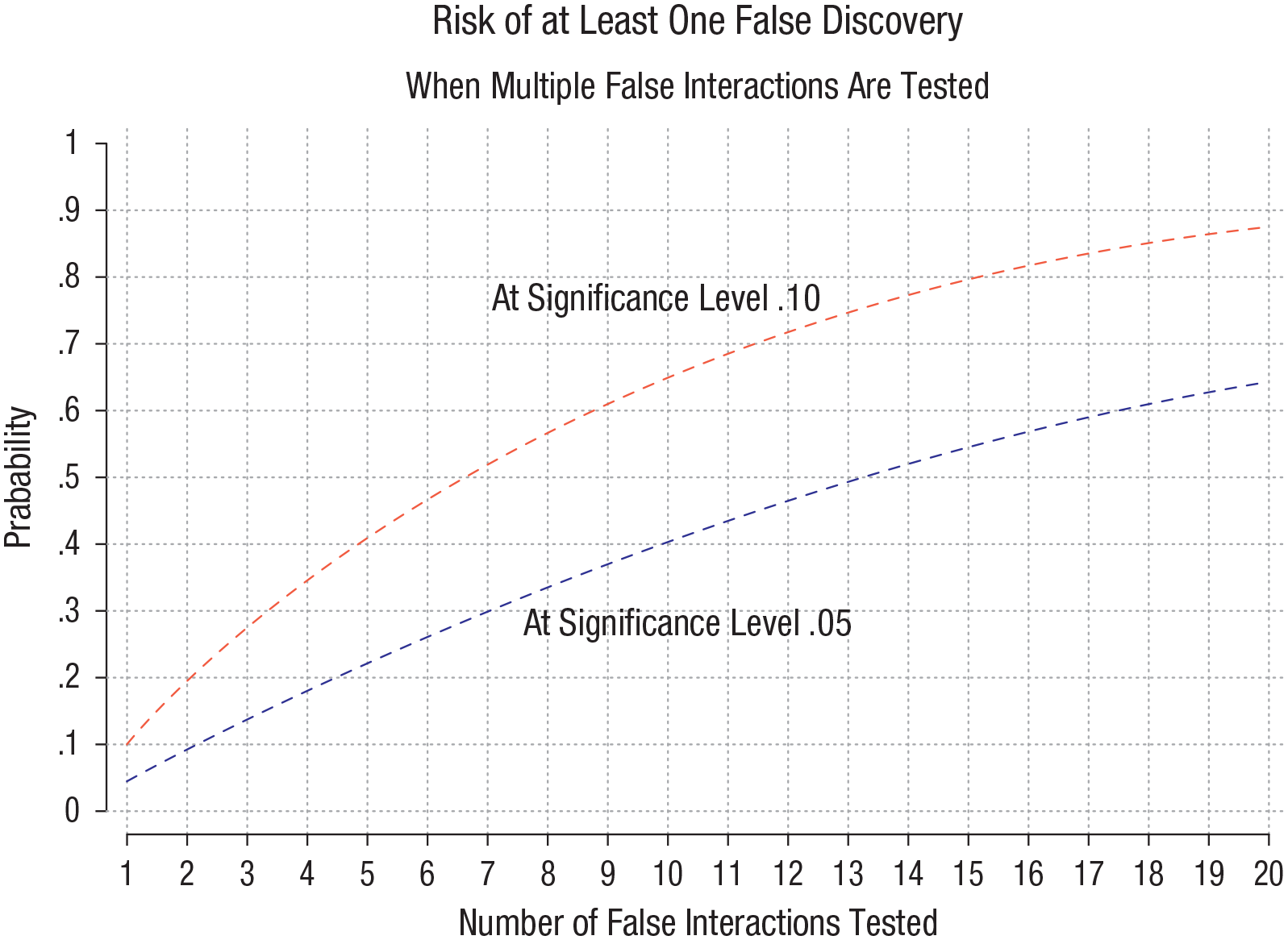
Risk of at least one false discovery when multiple false interactions are tested. As more false interactions are tested, the risk of a false discovery rises. This figure graphs the probability of at least one false discovery, which is 1 – (1 – a)k, where a is the significance level and k is the number of false interactions tested.
These observations are important because a single significant result, if highlighted in a study abstract, can be enough to get a study published. And investigators can practically guarantee a single significant result by testing enough interactions.
It is easy to find studies in which five interactions—or 20 or more—have been tested. For example, a treatment can interact with gender (two categories or more), race/ethnicity (two to six categories), weight status (overweight, obesity, normal weight), age, educational level, and many other characteristics. The number of potential interactions grows if three- and four-way interactions are permitted—as they often are, at least implicitly.
For example, in estimating the effect of physical-education classes on body weight, one study reported no effect except for boys in fifth grade (Cawley et al., 2013)—implying a three-way interaction between treatment, gender, and age. Another study reported an effect only for girls in kindergarten and first grade and only if they started the study overweight—implying a four-way interaction between treatment, gender, age, and initial weight status (Datar & Sturm, 2004).
Neither interaction replicated in later data (Bednar & Rouse, 2020), and both may have been false discoveries.
Recommendation 10: resist the temptation to test too many interactions when there is no main effect
Investigators who fail to find a significant main effect may be especially tempted to search for interactions. Such no-but heterogeneity does exist, but it is rare. True heterogeneity is generally smaller when there is little or no main effect (Olsson-Collentine et al., 2020).
In other words, investigators may be most tempted to search for heterogeneity when it is least likely to be present—“grasping for a positive straw in a negative haystack” (Berry, 2012). Investigators who search for no-but heterogeneity will test more false interactions and conduct lower-powered tests of true interactions. The result will be a higher false-discovery rate than would be typical if a strong and significant main effect were present.
Recommendation 3 (again): correct for multiple inferences
Our recommendation to avoid testing too many interactions stems from concerns about multiple inferences. We already recommended correcting for multiple inferences in our section on unexplained heterogeneity, but corrections have additional virtues when investigators try to explain heterogeneity through interactions.
Multiple test corrections do not just correct interactions that have already been tested—they also provide an incentive to avoid testing too many interactions in the first place. Once researchers agree to correct for multiple tests, then every interaction they test raises the bar that an interaction must clear to achieve significance. For example, if researchers test only five interactions, then they must multiply the smallest uncorrected p value by 5, and as long as the smallest uncorrected p value is less than .01, p will still be significant (less than .05) after correction. But if researchers test 20 interactions, then they must multiply the smallest uncorrected p value by 20, and unless the smallest uncorrected p value is less than .0025, every p value will be greater than .05 after correction.
By contrast, if investigators do not correct for multiple inferences, then every test increases our chances of finding a significant result—but many significant results will be spurious.
Recommendation 11: preregister interactions and do not report interactions selectively
Many investigators report interactions selectively—testing many interactions but reporting only a few in their article or reporting all interactions in their tables but mentioning only a few in their discussion and perhaps highlighting just one in their abstract. Multiple test corrections may be inadequate if they correct only for the number of interactions that are reported and not for the number of tests that were carried out.
The answer to this problem is preregistration. Before testing any interactions, we, as researchers, should preregister (e.g., on OSF) which interactions we plan to test and why. Later corrections should correct for all the interactions that were preregistered and not just those that were reported.
Recommendation 12: motivate interactions with causal mechanisms
One way to reduce the number of false interactions tested is to make sure that every interaction has a strong and clear motivation. The motivation should be linked to the mechanism by which the treatment is believed to work (Rohrer & Arslan, 2021). When researchers have a clear and consistent theory about why an intervention should work at all, they are better prepared to make clear and targeted predictions about when and for whom it will work best or worst. By contrast, when the treatment is a black box with no clear mechanism, it is harder to explain why the effects would be heterogeneous.
An example of a well-theorized interaction occurs in the literature on early reading, in which several studies have tested the hypothesis that phonics instruction is useful only for readers who lack fluent phonics skills. Students who have already mastered phonics will benefit little from further phonics instruction and can make better progress through independent and meaning-focused activities. Several small- to moderate-sized observational and randomized studies have confirmed the interaction between phonics instruction and initial skill level, and investigators have developed a screening test that can prescribe an effective mix of basic and advanced reading activities according to a student’s initial skill level (Connor et al., 2004, 2009; Connor & Morrison, 2016). Nevertheless, one large observational study failed to find any interaction between teachers’ instructional practices and children’s initial reading level (Chiatovich & Stipek, 2016). As this study illustrates, even well-motivated interactions do not always replicate, but they should at least offer a better chance of avoiding false discoveries.
By contrast, many investigations simply interact the treatment with whatever demographic characteristics happen to be available, such as age, race, poverty, income, or geographic location (Cintron et al., 2022). Although there are behaviors—such as attraction or discrimination—for which demographics may truly be the causal moderators of interest, in many settings, demographics are only weak proxies, at best, for the underlying social, psychological, or biological processes that might moderate a treatment’s effects.
For example, class-size research rarely specifies the mechanism by which small classes should help anyone learn (Pedder, 2006), and without a clear mechanism, it is hard to motivate the hypothesis that small classes would be better for Black children (the hypothesis that failed in Table 4) or children from families with low incomes. It is not hard to improvise a theory—maybe children in smaller classes get more differentiated instruction, or maybe classmates distract them less—but such theories would not motivate interactions between class size and race or poverty. Instead, if the mechanism were that smaller classes reduce distraction, one might expect larger effects for children with attention-deficit/hyperactivity disorder; or if smaller classes let teachers differentiate instruction, one might expect larger effects in classrooms in which children’s initial skill levels were more varied.
Recommendation 13: interpret interactions cautiously when covariates may be confounded
Note that diverse skill levels and distracting environments might be more common in classrooms serving larger proportions of Black students or students from low-income families. But such classrooms might not be more distracting or more varied in skill levels, and even if they were, race and poverty would be weak proxies at best—only slightly correlated with the psychological and instructional variables that actually moderate the effects of class size. When data are limited and mechanisms are vague, it is possible that apparent moderators in a study are actually proxies for unseen variables that really moderate the effect (Rohrer & Arslan, 2021). Researchers find themselves back in Cronbach’s (1975) “hall of mirrors.”
Note that the possibility of confounding disappears when a moderator is itself a treatment assigned at random. For example, in a psychiatry study that randomizes two treatments—say medication and therapy—there would be little ambiguity if there were an interaction suggesting that patients who received both medication and therapy benefited more than patients receiving either medication or therapy alone. But if a randomized treatment interacts with a trait or behavior that is not randomized—for example, if therapy were more effective for one gender than for another—then there is always the possibility that the observed moderator is confounded with some other variable that truly moderates the effect (Tipton et al., 2019). This is part of what Cronbach (1975) meant by the “hall of mirrors.”
Recommendation 14: center variables if you like, but it will not increase the power to detect interactions
Power to detect interactions is often low. As we wrote earlier, the main reasons are (1) that most interactions are small and (2) that many interactions are identified by small subsamples. But another reason is often suggested: An interaction XZ may be nearly collinear (i.e., strongly correlated) with one or both of the component variables X and Z. Collinearity can indeed inflate standard errors and reduce power. Nevertheless, collinearity is not a reason for low power to detect interactions, and steps to reduce collinearity do not increase the power to detect interactions.
To reduce collinearity, some scholars recommend mean-centering X and Z (i.e., subtracting their means) before calculating the interaction XZ (Aiken & West, 1991; Iacobucci et al., 2016; C. Robinson & Schumacker, 2009). Yet other scholars disagree, claiming that centering does nothing to reduce collinearity or shrink standard errors (Echambadi & Hess, 2007; McClelland et al., 2017). This disagreement has confused many applied researchers, who are left wondering whether they should center interacting variables or not.
What changes when we center variables in an interaction?
In Table 5, we clarify what does and does not change when interacting variables are mean-centered. Using data from Project STAR, the model regresses children’s school absences Y on class size Z and county flu prevalence X. The interaction XZ tests the hypothesis that, because children can catch flu from their classmates, having a small class might reduce absences more in counties where flu prevalence was high (von Hippel, 2021). Table 5 presents two versions of the model; one centers X and Z before calculating the interaction; the other model does not.
Linear Regression Predicting School Absences With Flu Prevalence Centered or Uncentered

Note: The model, fully described in von Hippel (2021), included child random effects, school fixed effects, and teacher-clustered standard errors (in parentheses). † p < .10, *p < .05. **p < .01.
Notice that centering did not change the interaction effect at all. The interaction’s point estimate, standard error, and p value are exactly the same whether variables are centered or not. These results are typical, and they mean that centering does not increase the power to detect an interaction (Afshartous & Preston, 2011; Iacobucci et al., 2016). Centering also did not change the model fit (R2), which was .0438 whether variables were centered or not.
But centering did change the estimates of the main effects. The estimated effect of class size changed a little, and the estimated effect of flu prevalence changed a lot. The coefficient of flu prevalence was cut in half, and its standard error and p value were cut by a factor of 4, turning a clearly nonsignificant estimate (p = .39) into one that was closer to significant (p = .09). The reason for the increased power was reduced collinearity. Before centering, the interaction had a .96 correlation with flu prevalence, but centering reduced this correlation to .00; that is why the standard error for the effect of flu prevalence shrank by a factor of 4. Centering also reduced the correlation between class size and the interaction, but not as much, from .21 to .02; that is why the standard error of the class size effect shrank only a little.
But centering did not change just the estimate of the main effects; it also changed what the main effects represent. Before mean-centering, the main effect of class size represented the effect of small classes in a community with no flu. But after mean-centering, the class-size slope represented the effect of small classes in a community with average flu prevalence. In a model with no interaction, these slopes would be the same, but in a model with interactions, they can be different because the effect of class size may be different at different levels of flu prevalence. The shape of the regression surface is the same, but centering means that the main effects are estimated at the middle of the surface rather than the edge.
So, should investigators center interacting variables or not? We would often recommend centering even though it does not increase power to detect an interaction. The advantage of centering is that it reduces the standard errors and p values of main effects while allowing researchers to interpret them as the main effect at the average value of the covariates. In many studies (but not all), investigators will prefer this interpretation over the alternative of estimating main effects at a covariate value of 0.
Unreliability usually is not a major reason for low power
Another reason sometimes given for interactions’ low power is that interactions are unreliable—that is, because much of the interaction’s variance is due to measurement error (Jaccard & Wan, 1995). There is a kernel of truth to this. The reliability of an interaction XZ is
Summary: how we unfooled ourselves about explained heterogeneity
In this section, we reviewed claims that several treatments had heterogeneous effects: the claim that small classes are more effective for children who are Black or have low incomes, the claim that physical education reduces weight only for children of certain ages and genders, and the claim that matching students’ race to teachers’ race increases the chances that Black students will be classified as gifted. In each case, we found that the result did not replicate and that the original study either did not estimate the relevant interaction or lacked adequate power to detect the interaction if it was present.
More broadly, our calculations suggested that a combination of inadequate power, inadequate theoretical motivation, and multiple inferences produced a situation in which 50% to 89% of significant interactions may be false discoveries. Although this sounds grim, it is not unrealistic. In the social sciences, only about 20% of significant interactions can be replicated (Altmejd et al., 2019; Open Science Collaboration, 2015). If research practices were typically sound, significant interactions would be more common in large samples with high power, but instead, significant interactions are more common in small samples with low power (O’Boyle et al., 2019).
These considerations suggest that many false interactions are being tested, many nonsignificant interactions are not being reported, and many interactions reported as significant are probably false.
We suggested that investigators can reduce false discoveries by estimating interactions instead of subgroup effects, limiting estimation to interactions that have adequate power and clear theoretical motivation, and correcting for multiple tests. If investigators follow these recommendations, future attempts to explain heterogeneity should be more trustworthy and replicable.
How Not to Let Models and Measurement Fool Us About Heterogeneity
Our recommendations so far can help us, as researchers, not to fool themselves about heterogeneity. Yet nearly all our recommendations so far pertain to general research practices—such as avoiding underpowered tests and correcting for multiple inferences.
Even if researchers follow sound practices, however, their models and measurements can sometimes fool them about heterogeneity. Researchers are most easily fooled when models are nonlinear or data might be measured on a noninterval scale. In this section, we make four final recommendations:
15. Check whether your interaction is present on every scale that might be used to measure the outcome variable Y.
16. Check for nonlinearity, floor effects, and ceiling effects.
17. When using logistic regression, check whether the interaction is present on both a probability and a log-odds scale.
18. When interpreting logistic, ordinal, or interval regression in terms of latent variables, check whether the interaction is still present if the latent variable has different variances for different subgroups.
We motivate these recommendations with concrete examples and illustrations.
Baseline misalignment: It is hard to compare effects on groups who start at different levels
Before making our recommendations, we note that they all stem in part from the problem of baseline misalignment. Baseline alignment—the requirement that the treatment and control groups have similar Y levels before treatment—is a common prerequisite for causal inference (Sekhon, 2009). If the treatment and control groups start at similar Y levels but finish at significantly different Y levels, then it is clear that there is a main effect of treatment.
When investigators search for heterogeneity, they often compare effects on groups whose Y values are not aligned at baseline. For example, they might compare the effects of an educational intervention on subgroups with higher or lower initial test scores or the effect of a job-training program on subgroups with higher or lower initial wages. When the groups being compared start at different Y levels—when they are misaligned at baseline—it can be challenging to tell whether effects on different subgroups are different. The challenges are especially acute when models are nonlinear or the Y variable can be measured in different ways.
Recommendation 15: check whether the interaction is present on every scale
When groups are not aligned at baseline, interactions can be sensitive to the scale on which the outcome Y is measured. On some scales, it may appear that the treatment effect is larger for Group 1; on others, it may appear that the effect is larger for Group 2. On still other scales, it may appear that the effect is equal for both groups (Domingue et al., 2022; Rohrer & Arslan, 2021).
As a simple example, suppose that a job-training program increased Group 1’s average earnings from $20,000 to $30,000 and Group 2’s average earnings from $30,000 to $40,000. On a dollar scale, there is no group by treatment interaction; treatment increased both groups’ earnings by the same amount: $10,000. But on a percentage scale, there is a group by treatment interaction; treatment improved Group 1’s earnings by 50% and Group 2’s earnings by only 33%. The effect on Group 1 also appears greater if one uses the logarithm of earnings.
Another example occurs in the literature on summer learning. Many studies have asked whether children in poverty fall behind other children more quickly during summer or during school. That is, does the effect of summer on learning interact with student poverty? The answer, it would seem, could shed light on whether schools make inequality better or worse. Yet the empirical evidence has been maddeningly inconsistent (von Hippel, 2019; von Hippel et al., 2018; von Hippel & Hamrock, 2019; Workman et al., 2022), and one reason is that results are sensitive to the scale on which learning is measured.
Figure 4 shows results from a longitudinal study in which reading tests were scored on two different scales (von Hippel & Hamrock, 2019). One scale measured how many questions children answered correctly; the other scale estimated children’s ability using item-response theory (IRT). On the number-right scale (Fig. 4, left), children in poverty fell behind other children during first grade, but on the IRT ability scale (Fig. 4, right), children in poverty caught up during first grade. The children were the same; the tests were the same—but changing the measurement scale flipped the time by poverty interaction from positive to negative (von Hippel & Hamrock, 2019, Table A5).

Interaction effects can depend on measurement scale. When scored on a number-right scale, children in poverty appear to fall behind during first grade. When scored on an item-response theory ability scale, children in poverty appear to catch up during first grade. Adapted from von Hippel and Hamrock (2019, Fig. 1).
The interaction changed sign not just because the scale changed but also because children in poverty did not start at the same place on the scale as other children. In addition, the relationship between the two scales was nonlinear. If the two scales had had a linear relationship—for example, if one measured the number right and the other measured the percentage right—then it would not have been possible to flip the interaction.
This example illustrates the importance of checking whether an interaction is robust to changes in scaling. If an interaction is sensitive to scaling, as this one is, investigators have two choices:
One can argue that it is unclear whether the interaction is positive or negative and refrain from interpreting it further.
Or one can argue that one scaling is better than another and that the better scale illustrates the true interaction.
In this example, the researchers argued that the IRT scale measures students’ skills better than the number-right scale (von Hippel & Hamrock, 2019). On the other hand, studies using different IRT scales can still produce inconsistent and nonreplicable results (Workman et al., 2022). Because of scaling and other issues, it remains unclear whether achievement gaps grow or shrink during school or summer and whether schools make inequality better or worse.
Recommendation 16: check for nonlinearity, floor effects, and ceiling effects
Interactions are often estimated with models that assume effects are linear. If effects are actually nonlinear, then fitting a linear model can produce the illusion of even if the effect is the same for every group.
Nonlinearity is not a concern when both the treatment and the moderator are discrete, but when either the treatment or moderator is continuous, then nonlinearity can be a concern.
Figure 5 gives two examples of nonlinear relationships in cognitive psychology. Figure 5a illustrates how reaction time decreases with practice. Reaction time decreases quickly at first and then more slowly as it nears the floor of 0, approximating an exponential curve or power law (Heathcote et al., 2000).

Common examples of nonlinearity in learning data. Group 1 is raw beginners, and Group 2 has prior experience. Both groups follow the same nonlinear curve, but if an incorrect linear model is fit, it will appear that there is a group by practice interaction because one group progresses more quickly than the other after starting the experiment. (a) Reaction time versus practice. (b) Accuracy versus practice.
Figure 5b illustrates how accuracy improves with practice. Accuracy improves quickly at first and then more slowly as it approaches the ceiling of 100%, approximating a logistic or sigmoid curve.
Such nonlinear relationships can create an illusion of interactions if investigators compare groups who start at different points on the curve. For example, one might compare the effects of practice on two groups—a group of raw beginners and a group with prior experience in the task. It may appear that the more experienced group improves less from practice—a group by treatment interaction—but the real issue is that the more experienced group is starting on a flatter part of the curve, nearer the floor or ceiling. They improve less because less improvement is possible, not because practice is less effective for them.
This highlights the necessity of plotting your data and not just assuming the data fit a linear model. If you find evidence of nonlinearity, it is better to use a curve that fits the data—say an exponential, power, or logistic curve—rather than assuming linearity. If no simple mathematical function fits the data well, then you can fit a flexible curve using splines, for example, or generalized additive models (Simonsohn, 2024).
The issue here is similar to the issues that arise from scaling. Indeed, the relationships in Figure 5 can be linearized if one transforms the scale of the outcome. For example, if one takes the log of reaction time, then its relationship with practice will be closer to linear, and it may be possible to estimate an interaction effect reasonably accurately with a linear model. Likewise, one can often linearize the relationship between practice and accuracy by applying a logistic transformation to accuracy. We say more about the logistic transformation in the next section.
Recommendation 17: in logistic regression, check if interactions occur in both probabilities and log odds
Perhaps the most common example of interactions being sensitive to scaling, nonlinearity, floors, and ceilings occurs when modeling the effect of some treatment on the chances of a binary outcome Y = 1, such as graduating high school, voting, or becoming overweight (Domingue et al., 2022; Embretson, 1996; Kang & Waller, 2005). Two models are commonly used.
A linear probability model predicts the probability p of Y = 1 as a linear function of X, Z, and the interaction XZ:

The coefficients represent the effect on the probability of graduation, and so on, of a 1-unit increase in X, Y, and the interaction XZ on the probability of graducation (or voting, or overweight).
Alternatively, a logistic regression model predicts the log odds ln((p / (1 – p)) as a linear function of the same variables:

The logistic model is harder to interpret but has the advantage of never predicting out-of-bounds values because log odds have no ceiling or floor.
If all the probabilities are in the middle of the range—say, between 0.2 and 0.8—then the linear and logistic models will give compatible results (Long, 1997; von Hippel, 2015). The logistic regression coefficients β will have an approximately linear relationship with the linear probability coefficients α, and if one model shows a significant interaction, then so will the other. The models will also give compatible results if the probabilities are all in a narrow range near the ceiling (a probability of 1) or near the floor (a probability of 0; von Hippel, 2017).
But if the starting probabilities are near the ceiling for one group and not for the other, then whether you see an interaction can depend on whether you put the results on a probability scale or a log-odds scale. In fact, interaction terms in logistic and linear models can disagree not just in significance but also in sign (Ai & Norton, 2003).
Figure 6 illustrates the problem with models that predict high school graduation from motivation and cognitive ability (inspired by Ganzach et al., 2000).
A linear model, predicting the probability of graduation, shows a negative interaction effect between a motivational “treatment” 7 and ability, suggesting that treatment was more beneficial for individuals with lower ability.
But a logistic model, using a log-odds scale, showed a positive interaction, suggesting that the treatment was most helpful to individuals with high ability.

Interactions on the Log Odds Scale Can Have Unintuitive Properties. Both graphs show the effect on graduation of a motivation intervention given to students with high versus low ability. The results are the same in both graphs, but the scale of the y-axis is different. (Left) This measures graduation on a probability scale and suggests a negative treatment by ability interaction: The benefit of the motivational intervention appears greater for students with low ability. (Right) This measures graduation on a log-odds scale and suggests a positive interaction, with a larger treatment benefit for students with high ability. (This example is inspired by Ganzach et al., 2000.)
This paradoxical result occurred for three reasons:
First, the high- and low-ability groups did not start at the same level. If the groups started with the same probability of graduation, the difference between the probability and log-odds scale would not matter; the interaction would have the same sign either way. But because the two groups started at different points, the choice of scale mattered for the interaction.
Second, the log-odds scale is a nonlinear transformation of the probability scale. If the two scales had a linear relationship, the change of scale would not affect the sign of the interaction.
Third, the log-odds scale is more sensitive to increases or decreases in probabilities near the ceiling of 100%. In this example, the high-ability treatment group had an almost 100% graduation rate. If neither group’s graduation rate went above 80% or so, then again, the interaction would not be so sensitive to the scale.
What scale should investigators choose between probabilities and log odds? One option is to make a philosophical judgment about which scale is right. Some researchers have argued that probabilities are a more “natural” metric (Long & Mustillo, 2021; Mize, 2019). They do not advocate the linear probability model, but they do argue that the results of a logistic regression model should be transformed back to a probability scale before any judgment about interactions is made.
Probabilities are indeed a more natural scale in many settings, but they also raise interpretive problems because of ceiling and floor effects. On a probability scale, higher-education interventions will often seem to have smaller effects on high-ability, highly motivated students whose probability of graduation would be near 100% without intervention. But does this mean that the interventions are less “effective” for such students, or does it simply reflect the fact that those students’ outcomes have little room for improvement on a probability scale?
And probabilities are not always the most natural scale. There are some behaviors, such as gambling, in which it is more natural to think in terms of odds or log odds.
There are also settings in which the purpose of logistic regression is not to estimate probabilities at all. We discuss those settings next.
Recommendation 18: in latent-variable models, allow for unequal variances between groups
There is another way to interpret logistic regression. Instead of interpreting it just as a probability model, one can view it as an attempt to estimate the parameters of a linear regression model:

where Y* is a latent variable that cannot be observed directly; instead, one can observe only whether Y* exceeds some threshold (Long, 1997). For example, suppose that Y* is adult body mass index (BMI), but all that is observed is a dummy variable Y indicating whether the adult is overweight (Y* ≥ 25) or not (Y* < 25). Then, one can estimate the parameters of the linear regression model for Y* by fitting a logistic regression model to Y.
It would appear that this approach can be used to estimate interactions. For example, if Z is a weight-loss intervention and X is a dummy indicating whether the patient is male or female, then if you conduct a logistic regression of overweight Y on X, Z, and the interaction XZ, the coefficient of the interaction will tell whether the intervention reduced BMI Y* more among men or among women—even if you cannot observe Y* directly but can observe only the dummy variable Y representing overweight.
But there is a catch. The approach assumes that the residuals e* of the latent linear regression have a logistic distribution with the same variance for men and for women. If this assumption is violated, then the approach can give misleading results (Allison, 1999). You can get a significant interaction when actually the treatment has the same effect on both groups. Or you can get no interaction when actually the treatment has different effects in each group.
Figure 7 illustrates the problem. Groups A and B have the same average Y* value before treatment and the same, somewhat higher, average Y* value after treatment. So, the treatment’s effect on Y* is the same for both groups; there is no interaction. However, because Group B has a larger residual variance than Group A, the probability of exceeding the threshold increases faster for Group B than for Group A. If you use logistic regression to model the probability of exceeding the threshold, you will get a substantial and possibly significant coefficient for the interaction XZ.

Differences in latent variance can create the illusion of interaction. Here, the latent means change by the same amount in Group A and Group B. But because the groups have unequal variances, the probability of exceeding the threshold increases by only about 10% for Group A and by 30% for Group B.
This problem here is distinct from the question of whether we use probabilities or log odds—either way, we can get misleading estimates for the interaction. It is also not a question of the two groups having different mean Y* values before treatment. For this example, we made sure that they had the same means. The problem is just that they have different variances.
The problem of unequal variances is not limited to logistic regression but crops up whenever one wants to model an unobserved continuous variable Y* from an observed variable that tells only whether Y* falls in certain categories or intervals. Examples occur in ordinal logistic regression, ordinal probit regression (Reardon et al., 2017; Williams, 2009, 2010), and interval regression (Bartlett, 2015). In all cases, assuming equal residual variances can lead to misleading estimates of interaction effects. The solution is to fit a more flexible model using software that allows for heteroskedasticity—that is, the possibility that different groups have different residual variances. Examples include the heteroskedastic ordinal probit model (Reardon et al., 2017) or the het option to the intreg interval regression command in Stata.
A related problem is that logistic and probit models assume that the residuals of the latent variable Y* have a logistic or normal distribution, but some latent variables do not. For example, the logistic and normal distributions are both symmetric, but the distribution of BMI is noticeably skewed, and asymmetry in the BMI distribution may affect conclusions of models that break BMI into categories such as normal, overweight, and obesity. Some software (e.g., the gintreg command for Stata) can fit categorical models that allow the underlying variable to have a skewed distribution (e.g., a gamma distribution), which fits BMI better. That too is worth trying before claiming an interaction.
Conclusion: Will The New Heterogeneity Revolution Succeed?
The prospect of a heterogeneity revolution is alluring. If it succeeds, investigators will be better able to target the right interventions to the right people in the right places at the right time. Patients will get more effective drugs with fewer side effects; educational interventions will reach the students who need them without wasting resources on students who do not. In field after field, a heterogeneity revolution could provide greater benefits with lower costs (Bryan et al., 2021).
But will the revolution achieve its potential? Our title is meant to evoke both a best-case and a worse-case scenario. The worst case was described in Townshend’s (1971) cynical lyrics to The Who’s hit song, “Won’t Get Fooled Again”: I’ll tip my hat to the new constitution, Take a bow for the new revolution . . . Then I’ll get on my knees and pray We don’t get fooled again.
As discussed in the introduction, the research community has been through a heterogeneity revolution before, and the results were disappointing. Reliable examples of heterogeneity proved hard to find. Many interactions involved small groups. Most interactions were small and hard to interpret. Several generations of researchers have been disappointed by their attempts to harness heterogeneity in pursuit of a more robust and useful social science.
Even in recent studies, interactions have been far less replicable than main effects; in fact, only one in five interaction effects has replicated successfully in new data. Many of the practices and incentives that produced spurious interactions one or two generations ago are still alive and well today. Investigators seeking publication and funding still have strong incentives to claim interactions where none exist (Franco et al., 2014), especially if there is little or no main effect. Underpowered analyses and multiple inferences are prevalent. Statistical methods that produce illusions of heterogeneity remain common, and methods that are more robust and less prone to illusion are not as widely known.
Yet our title also evokes a more optimistic scenario. In a 1974 commencement address that expressed skepticism about the usefulness and replicability of research in education, psychology, and criminology, the physicist Feynman (1974) articulated a key principle of scientific inquiry: “The first principle is that you must not fool yourself—and you are the easiest person to fool. . . . After you’ve not fooled yourself, it’s easy not to fool other scientists.”
The social sciences may have reached a level of maturity in which we, as researchers, are starting to learn how not to fool ourselves. There has been substantial progress in the 50+ years since the critiques of Cronbach, Feynman, and Townshend. Investigators have more appreciation for the prevalence of nonreplicable results and the research practices that produce them. Researchers take larger samples and use better research designs with more developed statistical methods whose properties are better understood. Preregistration and replication studies are becoming more common. Our goal in this article was to collect the practices and methods that are necessary to make any present or future heterogeneity revolution more successful.
Because authors competing for publication may be reluctant to adopt practices that reduce their chances of finding significant interactions, the field may need institutional reforms rather than trusting that individual authors will do the right thing. In clinical trials, regulators manage the risk of approving ineffective drugs by requiring statisticians to preregister analyses and correct for multiple inferences (Dmitrienko & D’Agostino, 2018). In genomics, a replication crisis led top journals to require authors to correct for multiple inferences and replicate analyses across multiple samples (Hewitt, 2012; Johnston et al., 2013).
Similar steps may be needed to address multiple inferences in psychology and other social sciences. If journals do not outright require authors to correct for multiple inferences, they can award badges to authors who do so voluntarily. Some journals already award badges to authors who preregister their analyses—which, among other things, helps to document how many hypotheses were tested and need to be corrected.
These steps will substantially increase the chances of a successful heterogeneity revolution. Yet researchers may have to temper their expectations for what such a revolution can achieve, at least in the short-term. In light of past disappointments, it may be rash to hope that in a few years researchers will develop a richly textured description of exactly when, where, and for whom every intervention will work or fail. It seems more realistic to hope that investigators may come to understand just a few circumstances that make a big difference in the effectiveness of a few interventions. And that will require not just better methods but also humility about what those methods can realistically accomplish. The heterogeneity revolution must go hand-in-hand with the open-science and replicability movements, with the combined aims of not only exploring sources of heterogeneity but also making sure that claims about heterogeneity can stand the test of time.
Footnotes
Transparency
Action Editor: Pamela Davis-Kean
Editor: David A. Sbarra
Author Contributions