
Abstract
Supervised machine learning (ML) is becoming an influential analytical method in psychology and other social sciences. However, theoretical ML concepts and predictive-modeling techniques are not yet widely taught in psychology programs. This tutorial is intended to provide an intuitive but thorough primer and introduction to supervised ML for psychologists in four consecutive modules. After introducing the basic terminology and mindset of supervised ML, in Module 1, we cover how to use resampling methods to evaluate the performance of ML models (bias-variance trade-off, performance measures, k-fold cross-validation). In Module 2, we introduce the nonlinear random forest, a type of ML model that is particularly user-friendly and well suited to predicting psychological outcomes. Module 3 is about performing empirical benchmark experiments (comparing the performance of several ML models on multiple data sets). Finally, in Module 4, we discuss the interpretation of ML models, including permutation variable importance measures, effect plots (partial-dependence plots, individual conditional-expectation profiles), and the concept of model fairness. Throughout the tutorial, intuitive descriptions of theoretical concepts are provided, with as few mathematical formulas as possible, and followed by code examples using the mlr3 and companion packages in R. Key practical-analysis steps are demonstrated on the publicly available PhoneStudy data set (N = 624), which includes more than 1,800 variables from smartphone sensing to predict Big Five personality trait scores. The article contains a checklist to be used as a reminder of important elements when performing, reporting, or reviewing ML analyses in psychology. Additional examples and more advanced concepts are demonstrated in online materials (https://osf.io/9273g/).
Keywords
Over the past decade, supervised machine learning (ML) has appeared with increasing frequency in psychology and other social sciences. In psychology, ML has been used to tackle such diverse topics as predicting psychological traits from digital traces of online and offline behavior (Kosinski et al., 2013; Stachl, Au, et al., 2020; Youyou et al., 2015), modeling consistency in human behavior (Shaw et al., 2022), or investigating the empirical structure of self-regulation (Eisenberg et al., 2019). This popularity can be traced to a number of features: a focus on prediction, which complements traditional methods that emphasize description and explanation (Shmueli, 2010); the flexibility to account for nonlinear patterns in large quantities of data (Kosinski et al., 2016); and an increase in the generalizability of research findings by evaluating predictive performance on new data (Yarkoni, 2022). Together, these features hold the promise of elevating the understanding of the processes that connect human behavior, cognition, and experience while being able to account for real-world complexity (Rocca & Yarkoni, 2021; Yarkoni & Westfall, 2017). However, the application, evaluation, and interpretation of ML-based analyses require new skills and acute awareness of its methodological challenges and limitations.
In this tutorial article, we aim to provide an intuitive but thorough introduction to the fundamentals of supervised ML for students, researchers, and educators in psychology. Our goal is to demystify ML and to help readers achieve their analytic goals. We introduce the most important ML concepts, which should enable readers to safely familiarize themselves with more complex methods in self-study. Our focus is exclusively on supervised ML (James et al., 2021; Kuhn & Johnson, 2013). We do not cover other branches of ML (e.g., unsupervised learning; see Murphy, 2022) and more advanced or specific topics (e.g., deep learning; see Goodfellow et al., 2016). We assume that readers are familiar with the free open-source statistical programming language R (Version 4.2.2; R Core Team, 2020), linear regression models, and their standard application in psychology or other social sciences.
In this tutorial, we present ML theory and application side by side. In each of four consecutive modules, we first introduce key theoretical concepts, prioritizing intuition and visualizations over mathematical formulas. Then, we apply the theoretical concepts in R while providing enough details for readers to understand which analysis steps to think about and how to adapt them to their own projects. Readers will benefit most from our tutorial by following our practical exercises on their own computers (but all major R outputs are included in our article). The tutorial covers a lot of content, and some concepts might seem complicated at first. We encourage readers to work through the tutorial at their own pace and revisit earlier sections to consolidate what they have learned. We added a short summary to the end of each module, which should make it easier to continue with the next module at a later time.
Before getting into the first module, we introduce the basic terminology and mindset of supervised ML and describe the data set and the software we use in our practical exercises. After setting the stage, in Module 1, we cover how to use resampling methods to evaluate the performance of ML models. In Module 2, we introduce the nonlinear random forest (RF; and its components regression and classification trees), a type of ML model that is particularly user-friendly and well suited to predicting psychological outcomes. Module 3 is about performing empirical benchmark experiments. Finally, in Module 4, we discuss the interpretation of ML models, including permutation variable importance measures, effect plots, and the concept of model fairness. At the end of the tutorial, we provide a single-page checklist that can be used as a reminder about important concepts and pitfalls when performing, reporting, or reviewing ML analyses in psychology. Beyond what we cover in the tutorial, we provide electronic supplemental materials (ESM) with additional examples and demonstrations of more advanced topics in an accompanying OSF repository. All materials for our tutorial, including our reproducible article, the data set, and the ESM can be found at https://osf.io/9273g/. We also uploaded our tutorial to Code Ocean (https://doi.org/10.24433/CO.5687964.v1), which provides the most convenient way to follow along with our exercises or the ESM directly in the browser without having to install any software.
The Terminology and Mindset of Supervised ML
Scientists often want to predict the value of some variable of interest using some other predictor variables. For example, in our own research, we were interested in predicting the personality trait score of a person (measured with a questionnaire) on the basis of their smartphone behaviors (recorded on their personal smartphone; Stachl, Au, et al., 2020).
Basic terminology
In supervised ML, the variable of interest (e.g., personality trait score) is often called “target,” and the predictor variables (e.g., smartphone behaviors) are called “features.” We use that terminology in this tutorial. Depending on the variable type of the target, supervised learning problems are typically divided into “regression” and “classification” tasks. In regression tasks, the target is continuous (e.g., personality trait score), whereas in classification tasks, the target is categorical (e.g., nominal: having an illness or not; ordinal: education level). For the classification task, there is a further distinction: The target can either have only two distinct values, which is called “binary classification,” or it can have more than two classes (e.g., country of origin), which is called “multiclass classification.” A visualization of simple regression and classification tasks can be found in ESM 2.1. We do not cover multiclass classification tasks in this tutorial, but most syntax can be easily adjusted for this setting.
To produce predictions for the target y when presented with concrete values for a series of features
For example, a simple predictive model is linear regression:
Predictive models differ with respect to their “flexibility.” A relatively inflexible model such as linear regression can account only for linear relationships, include manually selected linear interactions, and use a small number of features simultaneously. A flexible model such as the RF (Breiman, 2001a) promises to automatically learn nonlinear relationships and interactions while effectively dealing with a large number of features. If the true relationship between the features and the target is complex, a more flexible model has the potential to produce more accurate predictions when trained on enough data. Predictive models also differ with respect to their “interpretability.” The interpretability of a model refers to how easy it is to understand the relationships between feature values and the predictions of the model. Usually, there is a trade-off between model flexibility and interpretability. In more flexible models, interpretability is often more challenging or can be achieved only by applying additional methods because no simple model equation (cf. linear regression example) is available.
Predictive-modeling mindset
Talking about supervised ML often involves the application of relatively flexible ML models and, more importantly, a “predictive mindset” when performing data analysis. This mindset is sometimes at odds with how most psychologists were trained to apply statistical models, mostly limited to generalized linear models such as linear or logistic regression. Such “classical modeling” approaches have been described with many names, such as “data,” “descriptive,” and “explanatory” modeling (Breiman, 2001b; Shmueli, 2010). The classical approach aims to understand and model the concrete relationships between variables. Given theoretical knowledge or previous work, a statistical model with a specific relationship (e.g., a conditional linear association) is assumed that describes how the data were produced in the population. Appropriate model-fit indices such as
In supervised ML, researchers usually do not make any explicit assumptions about the data-generating process in the hope that the models can learn the specific functional relationship between the features and the target automatically. In contrast to evaluating the trained model on the same data set, which is what is usually done in classical modeling, supervised ML seeks to quantify the predictive performance of models regarding how well they can predict new, previously unseen observations. Appropriate performance measures that define what is a good prediction are carefully selected according to the intended model application instead of being derived from an explicit data model. After model evaluation, the focus is on concrete predictions, and the trained model parameters are often of secondary interest or not considered at all. Two (idealistic) assumptions are necessary for a trained model to make accurate predictions for new observations: First, all observations (those used to train the model and those used to evaluate the model) have to be randomly drawn from the same population. Second, when making predictions, the relationship in the population has not changed since the model was trained. Of course, predictions can also be computed for observations from a different population. However, a realistic estimate of predictive performance in this case requires reevaluating the model on data from this new population.
To get to the core of ML, it is important to embrace this predictive mindset when performing data analysis in an ML framework; this requires a thorough understanding of model evaluation in supervised ML. For example, how do researchers quantify the predictive performance of models regarding how well they can predict new, previously unseen observations? That is why we dedicate Module 1 exclusively to this topic.
Summary of the terminology and mindset of supervised ML
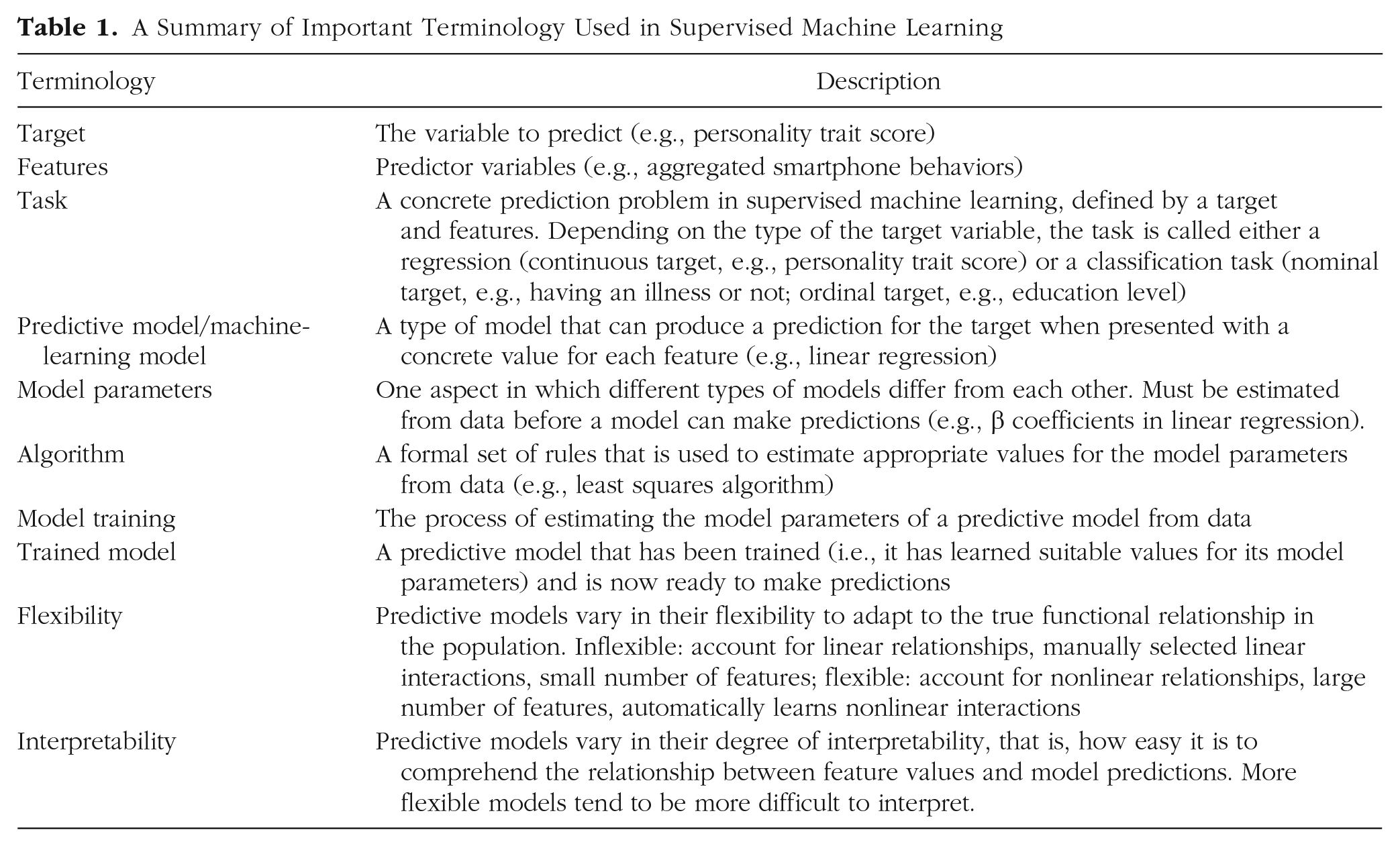
In the first section, we set the stage for the main modules of our tutorial by introducing the basic terminology of supervised ML and helping readers to adopt a predictive mindset that focuses on predicting new, unseen observations. Because ML uses a different language unfamiliar to psychologists, we summarized the most important terms in Table 1 to assist readers while working through the rest of the tutorial. Before we start with Module 1, we shortly introduce the data set and the software packages, which are used in the Practical Exercises 1 to 4.
A Summary of Important Terminology Used in Supervised Machine Learning
Data Sets Used in Practical Exercises
Throughout the tutorial, we use the publicly available PhoneStudy behavioral-patterns data set, which has been used to predict human personality from smartphone-usage data (Stachl, Au, et al., 2020). Subsets of these data have also been used in a number of other publications (Au et al., 2021; Harari et al., 2020; Schoedel et al., 2018, 2020; Schuwerk et al., 2019; Stachl et al., 2017; Sust et al., 2023). The data set contains self-reported questionnaire data of personality traits measured with the German Big Five Structure Inventory (five factors and 30 facets; Arendasy et al., 2011), demographic variables (age, gender, education), and behavioral data from smartphone sensing (e.g., communication and social behavior, app usage, music consumption, overall phone usage, day-nighttime activity). The smartphone sensing data were recorded for up to 30 days on the personal smartphone of 624 study volunteers, bundled from several smaller studies (e.g., Stachl et al., 2017). Here, we use the data set for the following regression task: We predict the continuous personality trait score for the sociability facet of the trait extraversion using 1,821 features of aggregated smartphone-usage behavior (e.g., a person’s average number of telephone calls at night). Demonstrating ML concepts on a real data set is important for getting a feeling for common obstacles, but it also means that not all context-specific details can be discussed exhaustively. More details on the data set can be found in Stachl, Au, et al. (2020), along with an in-depth discussion of the research question and interpretation of the final results. We use the PhoneStudy data set to demonstrate the main ML methods introduced in each module. However, when the data set is too complex to allow for an intuitive illustration of some theoretical concepts, we use two more simplistic open data sets from the general ML literature: AmesHousing and Titanic. 1
Software Used in Practical Exercises
Throughout the tutorial, we use an ML framework that provides a unified interface to train, evaluate, and interpret ML models, which helps users to write modeling syntax that is shorter and less error-prone. There are several popular frameworks available in the main coding languages (e.g., tidymodels in R, Kuhn & Wickham, 2020; scikit-learn in Python, Pedregosa et al., 2011). Here, we use mlr3 (Lang et al., 2019) and DALEX (Biecek, 2018): mlr3 (and its companion packages) provides a standardized interface to perform ML analyses in the open-source statistical programming language R (Version 4.2.2; R Core Team, 2020); DALEX provides functionality for model interpretation. A detailed tutorial on mlr3 is available as a free e-book (Bischl et al., 2023) at https://mlr3book.mlr-org.com/. The mlr3 package is written in the object-oriented programming system R6 (Chang, 2021), which is why some mlr3 syntax looks unfamiliar to readers used to base R. In ESM 2.2, we highlight possible sources of error for users unfamiliar with R6 and give advice on how to effectively look up information in the extensive mlr3 documentation.
Module 1: Performance Evaluation
Performance evaluation in theory: basics
In the first module of our tutorial, we cover the most important concept of predictive modeling: performance evaluation. Responsible use of ML mandates a thorough evaluation of the quality of a trained predictive model on the basis of the magnitude of error that can be expected for new (unseen) data from the same population. What does this mean? Imagine we have trained a predictive model (i.e., the model is ready to make predictions). Before we apply the model in practice, we want to know how well it will predict observations in our practical application, where the true target values are not available. So the key question is how to quantify the quality of models.
The bias-variance trade-off
The so-called bias-variance trade-off can be a helpful mental model, which we introduce with the following thought experiment: We have two models of different flexibility, and they greatly differ in their predictive performance (i.e., how well they predict new unseen data). What factors influence the performance of a predictive model in theory?
The “expected prediction error” of a predictive model consists of “bias,” “variance,” and “noise” (James et al., 2021). A metaphorical illustration is given in ESM 2.3. Before we continue with a graphical illustration, consider the following simplified definitions: Expected prediction error is the average prediction error we would expect when repeatedly fitting the same ML model on many samples of a certain size and measuring the prediction error on the basis of new samples with a large size. We assume all samples are randomly drawn from the same population of interest. Bias is the deviation of the average prediction from the true value. Variance is the variability of predictions based on different samples. Noise is the irreducible error of the true model in the population.
Counterintuitively, bias and variance are not attributes of a single trained model but refer to how a particular ML model would perform when fitted to repeated samples from the same population (e.g., collecting multiple samples of German psychology students). Figure 1 illustrates the bias-variance trade-off. The black line represents the population model, from which we draw samples of size
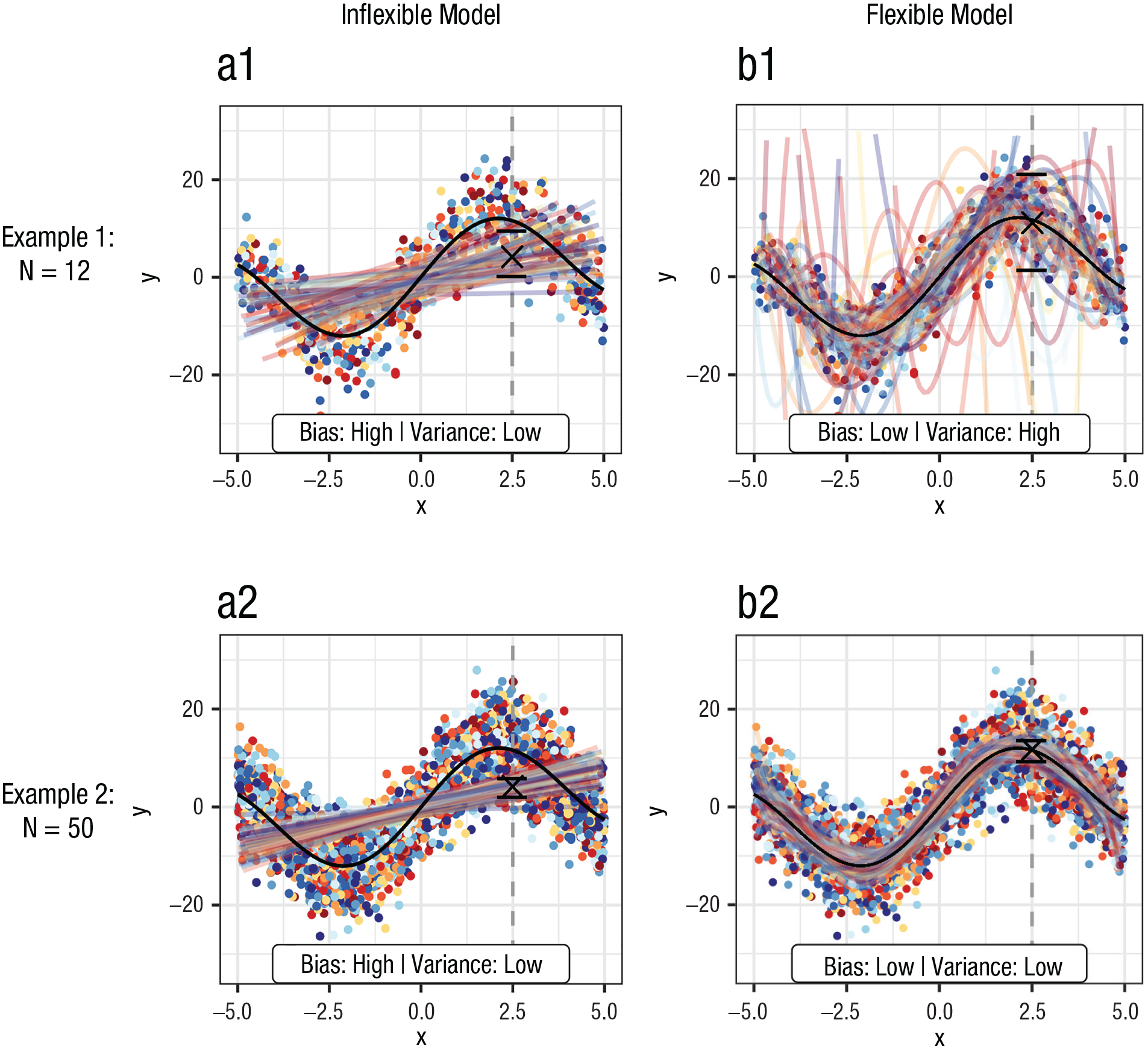
Visualization of the bias-variance trade-off by fitting machine-learning models with different flexibility on multiple samples (one color per sample) from a nonlinear population model (black). Left column = inflexible (linear) model; right column = flexible (seventh-degree polynomial) model; first row = 60 samples with N = 12 each; second row = 60 samples with N = 50 each. Mean (cross) and 0.1 and 0.9 quantiles (bars) of model predictions are displayed at x = 2.5 (vertical line).
To better “see” bias and variance, we ask our readers to visually focus on Example 1, where we use small sample sizes. If we pick a single point on the x-axis (e.g.,
Figure 1 also illustrates that the bias-variance trade-off can be heavily influenced by sample size if we compare Examples 1 and 2. Both the inflexible and flexible models are trained on small samples (
To conclude, when we aim to quantify predictive performance or to compare different ML models, it is helpful to keep the bias-variance trade-off in mind. The goal of supervised ML is always to strike a good bias-variance trade-off—to find a predictive model with both low bias and low variance. However, ML cannot escape from a general principle in statistics: More flexible models with weaker assumptions about the true functional relationship require more data to be effective.
Performance measures
In the previous section, we used vague definitions of prediction error and predictive performance to give an intuition of what it means for a predictive model to perform well. However, before we can evaluate a given ML model in practice, we need concrete definitions of prediction error for model predictions. Let us assume that someone provides us with a set of true target values and the corresponding predictions of a model. Without knowing anything about where these predictions come from, how would we quantify how good the predictions are? The first step of model evaluation is thus to select appropriate performance measures depending on the task type (i.e., regression or classification), research questions, and whether we want to use standard measures or we have expert knowledge leading to custom measures relevant for our specific model application.
Regression tasks
Performance measures for regression quantify a “typical” deviation from the true target value. The default measure is the mean squared error (MSE),
In the social sciences, the coefficient of determination (
Classification tasks
Measuring classification performance is often less straightforward compared with regression tasks. We consider only binary classification in which the target has two possible values (coded as 0 and 1 by convention) but there are comparable performance measures for multiclass classification (Ferri et al., 2009). The simplest idea to construct a performance measure is to compute the proportion of misclassified observations, which results in the mean misclassification error (MMCE),
Confusion Matrix
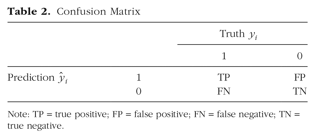
Note: TP = true positive; FP = false positive; FN = false negative; TN = true negative.
From the context of diagnostics and assessment, many psychologists are familiar with the sensitivity, also called true positive rate or recall:
Resampling strategies for model evaluation
In ML, it is always the predictive performance on new observations that is of practical and theoretical interest. Thus, we want to know how well a model trained on a specific data set will predict new, unseen data (out-of-sample performance). The ideal approach would be to collect a new sample from the same population. However, this approach is often not feasible in practice. A naive alternative would be to estimate predictive performance on the basis of the same data used to train the model (in-sample performance). Unfortunately, this procedure can lead to an extreme overestimation of predictive performance, which we demonstrate later. Too flexible models can perfectly predict all observations they have been trained on, but the predictions for new observations can be disastrous. A better approach for model evaluation is to use resampling methods, which are a smart way of recycling the available data to estimate out-of-sample performance. The general principle is to use the available sample to simulate what happens when the trained model will be applied on new observations in a practical application. To produce a realistic estimate of expected performance, resampling methods must ensure a strict separation of model fitting and model evaluation. This rule implies that different data must be used for training and testing the model.
The idea behind resampling
One of the simplest resampling strategies is to randomly split the data into a training set and a test set. The training set is used to train the model, and the test set is used to compute predictions and estimate predictive performance. Imagine we have a data set from a random sample consisting of a target y and a set of features X, as displayed in Figure 2. We use the entire data set to train an ML model, which we want to use in a practical application (Fig. 2a). We call this “full model” (shown in red in Fig. 2) because it used all of the available data. The full model learns a functional relationship between the features and the target. For new observations (i.e., when we apply the model in practice), the feature values
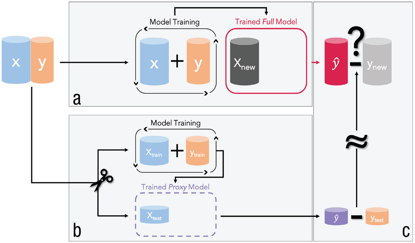
A visualization of how predictive performance is evaluated in supervised machine learning. (a) The training of the full model (red), which can later be used in an application (i.e., to predict new observations). The predictive performance of the full model is estimated by resampling. For this purpose, a proxy model (purple) is trained on (b) a training set, and the predictive performance computed on (c) the corresponding test set is used as an estimate of the predictive performance of the full model.
Why is it necessary to separate training and test data rather than computing the performance on the basis of the complete data set that we used to train the full model? Flexible ML models sometimes adjust to a set of given data points too closely, a phenomenon that is often called “overfitting.” If a model overfits to the data, it learns sample-specific patterns (“fitting the noise”) that will not generalize to new samples from the same population. Overfitting can also be thought as “learning something by heart”: The model exactly recognizes each observation it has been trained on but cannot transfer any information to new observations it has not seen before. We show later that especially for flexible ML models, in-sample performance is useless to judge a model’s performance on new data.
Figure 3 illustrates the concepts of overfitting and model evaluation. In Figure 3a, points were simulated from a nonlinear population model (dotted line) and randomly split into a training set (black dots) and a test set (framed dots). Note that because of the irreducible noise in the data-generating process, even the true population model would not predict observations perfectly. Three models of varying flexibility were fitted to the training set: polynomial regression models with Degrees 1 (linear model; green), 3 (orange), and 8 (purple). The green model clearly underfits. It is not flexible enough to approximate the population model and makes bad predictions for both training and test observations. The purple model overfits because its flexibility is too high. It almost perfectly interpolates all training observations, but the deviations from the test observations can be quite high. In contrast, the orange model seems to have optimal flexibility and closely approximates the population model. It roughly predicts training and test observations equally well. In such a simple example with only one feature, it is possible to visually identify the model with optimal flexibility. However, with more features, this becomes rapidly unfeasible because visualizing more dimensions is difficult. Fortunately, we can always try to determine the optimal model on the basis of the test-set performance. In Figure 3b, we show how training and test MSE were computed on the simulated data from Figure 3a for polynomial models with flexibility ranging from Degree 1 to Degree 9, which includes the three models displayed in Figure 3a. Remember how to compute the (training) test MSE: For each observation from the (training) test set, take the squared vertical difference between the point and the model prediction; then compute the mean of all squared differences. The trajectories of training and test performances along the axis of model flexibility show a characteristic pattern: Prediction error in the training set decreases with increasingly flexible models and almost reaches 0 (perfect interpolation) for Degree 9. We saw in Figure 3a that models with extremely high flexibility overfit and perform poorly on new observations. Hence, it becomes clear that we cannot use the training performance to select the optimal model. In contrast, prediction error in the test set first decreases until Degree 3 but then increases again. This reflects our observation from Figure 3a that both very low and very high flexibility is not ideal to achieve good predictions for new observations. In the bias-variance framework, bias decreases with flexibility, and variance increases. The optimal trade-off in this example seems to be a degree of about 3. To conclude, if we have to choose between different types of models or model settings, we generally select the model with the best performance on the test set (here, the model with the lowest MSE). In theory, we could favor models with lower flexibility among models with comparable test-set performance. However, this is usually not the default in practice. 2

(a) Observations drawn from a nonlinear population model (dotted line) divided into a training (black dots) and a test set (framed dots). Three models of varying flexibility (polynomials of Degrees 1 in green, 3 in orange, and 8 in purple) were fitted to the training set. (b) Relationship between model flexibility (polynomials of Degrees 1 to 9) and predictive performance estimated with training and test mean square error (MSE). Performance estimates are computed using the data from Figure 3a.
Different types of resampling strategies
In the previous example, we worked with the most simple resampling strategy of randomly splitting the data into a training set and a test set. This strategy is also termed the “holdout” estimator. An important practical issue when using the holdout estimator is the ideal proportion of data to put into the training and the test sets. The full model is always based on more observations than the proxy model that is fit to only the training set. Because model quality increases with sample size, test-set performance will (on average) be an underestimate of the true performance of the full model. The larger the training set, the smaller this negative bias is. The test-set performance is only a point estimate of the true predictive performance of the full model. Thus, the variance of this estimate is also important. The larger the test set, the smaller the variance of the performance estimate is. This is a dilemma because it is obviously not possible to maximize the size of training and test sets simultaneously (without collecting more data in the first place). We can think of this as the bias-variance trade-off of the holdout estimator, which should not be confused with the bias-variance trade-off of ML models we discussed earlier. 3 The trade-off strongly depends on the size of the training and test sets, but there is no single ratio that is optimal in general. Rules of thumb (see James et al., 2021) typically suggest to use two thirds of the full data for the training (large enough to learn well) and one third for the test set (large enough for stable performance evaluation).
In some ML settings in which the amount of data is not a problem, the holdout estimator is sufficient to achieve reasonable performance estimates. For extremely large (think of “Google sized”) data sets, the predictive performance of most ML models saturates (i.e., the performance no longer improves with increasing amounts of data), and the size difference between the training and the full data sets becomes irrelevant. At the same time, the variance of the performance estimate computed on the test set will be so small to be almost negligible. In the social and behavioral sciences, researchers usually face the situation that data are scarce and their collection are costly and time-consuming. For such smaller data sets, the performance difference between the full model and the proxy model and high variance of performance estimates from small test sets negatively affect the quality of holdout estimates. More elaborate resampling strategies, try to improve on the holdout estimator by recycling the data in a smarter way. You can optimize the partitioning of the data set by performing several splits into training and test sets and aggregating the resulting performance estimates. The most common resampling method is k-fold cross-validation (CV; Kohavi, 1995). Bischl et al. (2012) provided a good overview of CV and alternative resampling techniques such as repeated CV, leave-one-out CV, bootstrap, or subsampling.
In k-fold CV, the data set is randomly partitioned into k (roughly) equally sized parts. Each part is used as a test set exactly once, and the remaining parts are combined into a larger training set. The CV estimator is the average of the performance estimates from the k test sets. Figure 4 is a visualization of 3-fold CV (i.e., the data are randomly divided into three parts). In the first fold, a proxy model is trained on the combined data from Parts 1 and 2, and Part 3 (Fig. 4, green) is used to compute predictions and calculate the performance measure. In the second fold, Parts 1 and 3 form the training set, and Part 2 forms the test set. Finally, in the third fold, Parts 2 and 3 form the training set, and Part 1 forms the test set. The performance estimates from the three test sets are aggregated by the arithmetic mean (other aggregation functions such as the median are also possible). Note that each observation from the complete data set will be used exactly once (it is either in Test Set 1, 2, or 3) to make a prediction and thus to contribute to the final performance estimate. For each prediction, the observation in question was never used to train the model making that prediction. However, each observation belongs to two of all three training sets and thus is used several times to train proxy models. Compared with holdout, CV reduces the bias by increasing the size of the training sets and reduces the variance by aggregating several test set performances.
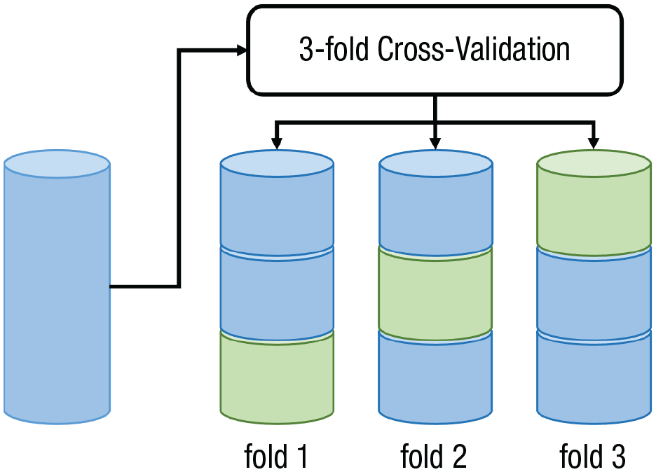
Visualization of the principle behind 3-fold cross-validation.
A simple intuition for those advantages can be given for 2-fold CV, in which the training and the test sets have the same size. Imagine a holdout estimator in which the training and the test sets have the same size. The model is trained on the first part, and performance is tested on the second part. However, if we switched the training set and test set, the resulting performance estimate would be of exactly the same quality. The size of the training set (i.e., the bias) is similar, and the size of the test set (i.e., the variance) is also the same. In addition, both performance estimates are independent (set assignments were random, and sets do not overlap). Thus, it is intuitive that the 2-fold CV estimator, which computes the mean across both test-set performances, will have similar bias but lower variance than each of the two holdout estimators. Unfortunately, the intuition breaks down for
Excursus on sample size
We want to conclude the section on performance evaluation with a comment on sample size. By far, the best strategy to improve the performance of predictive models for some application is to increase the amount of available data: For larger samples, (a) the variance of model predictions is lower, (b) the potential for flexible models with low bias is higher, (c) the danger of overfitting is lower, (d) the more features can be used effectively, and (e) the precision of estimates of predictive performance increases.
Practical Exercise 1: performance evaluation with k-fold cross-validation
Compute in-sample performance estimate
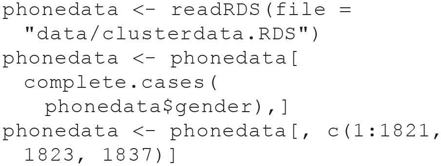
In our first practical exercise, we demonstrate how to use mlr3 to fit a standard linear regression model to the PhoneStudy data set by predicting the sociability personality-trait score on the basis of all variables of aggregated smartphone-usage behavior. Then we compare in-sample and out-of-sample predictive performance using
First, we load the PhoneStudy data set and remove some administrative variables we do not use in our tutorial. We also remove four participants who did not report their gender:
We load the mlr3verse - R package (Lang & Schratz, 2021), which conveniently loads mlr3 and the most important companion packages. Then we create a task object with a unique ID (Sociability_Regr), which is mlr3’s way to store the raw data along with some metainformation for modeling. In mlr3, a task defines a certain prediction problem, here, supervised regression with the sociability trait score (named E2.Sociableness in our data set) as the target: 7
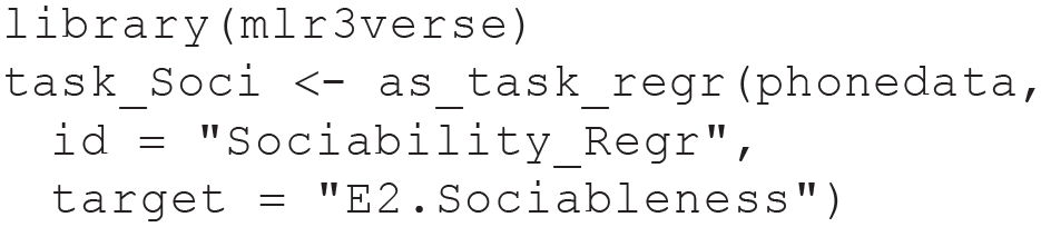
The metadata can be displayed by printing the task object (type task_Soci). When training a model on a task, mlr3 by default uses all variables except the target as features. We do not want to use gender as a feature, although we want to check our models for gender fairness in a later module. Therefore we remove gender from the set of features but keep it within the task object:
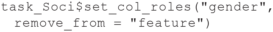
We recommend to always doublecheck which variables are really intended to be used as features (you can get the full list of feature names with
Next we create a learner object to specify an ML model to apply later. mlr3 does not implement its own ML models but links to available implementations in other R packages. For example, the ID regr.lm links to the ordinary lm function in the stats package. You can find a list of mlr3 IDs for the most popular ML models in the mlr3 e-book (Bischl et al., 2023):

We try to train (i.e., estimate model parameters) the learner on the task. In mlr3, objects have “abilities” (also called “methods”) that can be applied with the following $-syntax (here, the train method of the learner object is used to train the learner on a specified task):
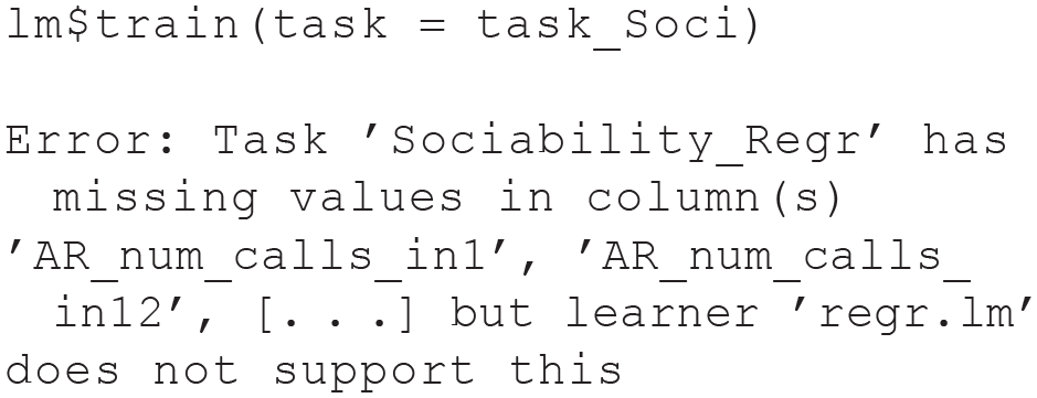
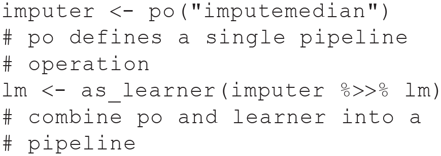
Unfortunately, this fails because there are missing values in the data set, and regr.lm cannot handle them. We use mlr3pipelines (Binder et al., 2021) to build a simple analysis pipeline, called GraphLearner in mlr3 (a learner consisting of several consecutive analysis steps that can be visualized as a graph), that automatically replaces missing values with the median of the respective training set (i.e., median imputation) before fitting our linear model. We do not recommend using mean or median imputation in real applications. 8 A tutorial on how to build more complex analysis pipelines with the mlr3pipelines package can be found in the mlr3 e-book (Bischl et al., 2023):
Now, training the augmented learner on the task works just fine:

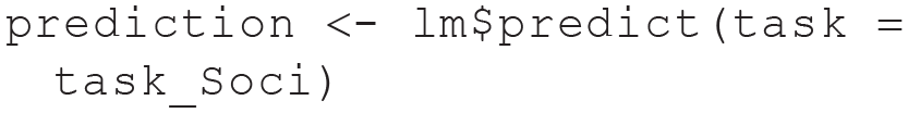
The previous line trained the model and automatically stored it inside the learner object. One great advantage of mlr3 is that we can use the same modeling functions for ML models from different R packages without having to remember the peculiarities of their modeling syntax. We can use the trained model to make predictions, which we have to store in a separate object: 9
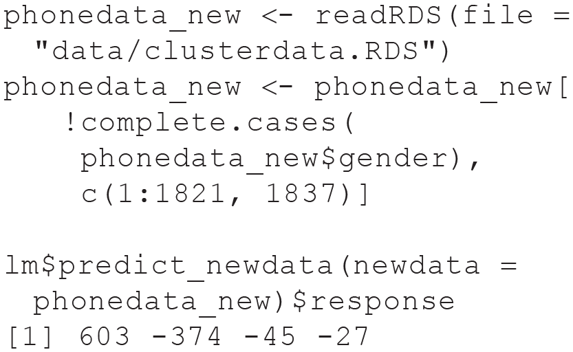
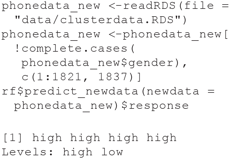
We just predicted the same data that we already used for model training, but we could also compute predictions for new observations. In the Sociability task, we did not include four individuals with missing values on the gender variable. Because we do not use gender as a feature here, we can treat these individuals as new data and predict their sociability score with
With this functionality, it would be possible to use the model in a practical application. However, it would be irresponsible to apply any predictive model for which the expected predictive performance is unknown. Therefore, we now demonstrate how to evaluate predictive performance with mlr3.
If we wanted to compute in-sample performance on the basis of the predictions for all observations included in our task (which we stored in
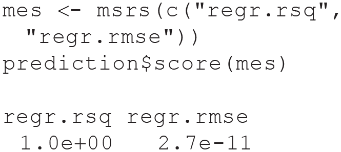
The performance on the training data is almost perfect.
Compute out-of-sample performance estimate
Next we want to use CV to compute an out-of-sample performance estimate. We specify a resampling strategy (here, 5-fold CV). You can run

The
When we compare the out-of-sample with the in-sample estimates, we realize that the predictions of our model are expected to be really bad. This might be no surprise to many readers because we used ordinary linear regression with 620 observations and 1,822 predictor variables, which results in an unidentified model. As a consequence, the
Performance evaluation in theory: advanced
Model optimization
Our first exercise demonstrated how to estimate the predictive performance of a simple predictive model with CV. However, predictive modeling in practice often entails a series of model decisions (or researcher degrees of freedom; see Wicherts et al., 2016) that have to be considered when estimating predictive performance: (a) hyperparameter tuning, (b) preprocessing, and (c) variable selection.
Many types of ML models have hyperparameters, which are parameters that are not automatically estimated during the training process by the estimation algorithm. However, because they can have a big impact on predictive performance, optimal values have to be chosen in a data-dependent way. Tuning hyperparameters (i.e., finding optimal configurations) typically works similarly to our model-comparison example in Figure 3. The degree of the polynomial can be seen as a hyperparameter of a general polynomial regression model. To find the optimal hyperparameter setting, we again use resampling (e.g., a single test set or CV) to estimate predictive performance for different hyperparameter settings, select the hyperparameter value with the best test-set performance, and choose the selected value when training the full model on the complete data set. Preprocessing operations can also have hyperparameters, which can be tuned in the same way as hyperparameters of ML models. A simple example for a categorical hyperparameter would be whether to use the mean or the median for data imputation. Regarding variable selection, sometimes it can be a good strategy to not include all possible features in a predictive model but only a subset of particularly informative features. A simple method for regression tasks is to compute the Pearson correlation for each feature with the target and use only the features with the highest target correlations when training the full model. Note that the number of features selected is a hyperparameter of this variable-selection strategy, which could again be tuned with CV.
Nested resampling
Modeling decisions such as those mentioned above are often implemented in a way that makes data-dependent choices before the full model is trained on the entire data set (e.g., predictive performance of mean and median imputation is compared on a test set to decide which method to use for the full model). To estimate predictive performance correctly when data-dependent choices have been made, it is of utmost importance to focus on the complete modeling pipeline, which contains the hyperparameters of the ML model and all previous or consecutive steps such as feature preprocessing or variable selection. For each training set in the resampling process used to estimate predictive performance, all data-dependent model decisions have to be repeated in exactly the same way as they are performed when producing the full model (which will actually be used to compute predictions in practical applications). This procedure entails the possibility that in some training sets, different hyperparameter settings are chosen than in the full model. That phenomenon might seem unintuitive, but it is unproblematic.
If data-dependent model decisions are not repeated within resampling, the predictive performance of the full model can be grossly overestimated. This mistake is most commonly observed when tuning the hyperparameters of ML models: First, researchers try out different hyperparameter combinations to find the setting with the best predictive performance in sample or with resampling. For example, in accordance with Figure 3, they determined that a third-degree polynomial seems optimal. Then they use this hyperparameter setting to train a full model on the basis of the complete data set, which is fine. However, to estimate the predictive performance of their full model, they run holdout or CV but use the degree setting from the full model in each training set. To obtain a realistic performance estimate of their full model, they should instead have repeated the tuning process of finding the optimal polynomial degree in each training set.
If modeling decisions require resampling themselves (e.g., hyperparameter tuning), correctly estimating the predictive performance of such a modeling pipeline results in nested resampling loops. We do not need nested resampling for the practical exercises performed in this tutorial because we do not employ hyperparameter tuning. However, we explain nested resampling in ESM 3.2, which also contains a full example with code on how to tune hyperparameters in mlr3.
Variable selection
Another prevalent example of overoptimistic predictive performance estimates by not considering data-dependent model decisions in performance evaluation is biased variable selection (Varma & Simon, 2006). Researchers might be interested in a sparse, interpretable model and want only to include a certain maximum number of features. Or they hope that a reduced feature set that contains most of the “signal” might increase predictive performance because the ML model is not distracted by other “noisy” features. Both can be valid reasons to perform variable selection, but variable selection is often evaluated with the following flawed procedure (James et al., 2021): First, researchers determine a limited number of features with the best predictive performance in sample or with resampling. They then use the selected features to train a full model on the basis of the complete data set, which is fine. However, to estimate the predictive performance of their full model, they run holdout or CV but include the features selected by the full model in each training set. To obtain a realistic performance estimate of their full model, instead, they should have repeated the variable-selection process of finding the optimal features in each training set before evaluating on the respective test set.
Biased variable selection invalidates many applied ML articles in the social sciences and threaten the replicability of this literature (for a discussion of biased variable selection in early studies of predicting personality traits with mobile sensing features, see Mønsted et al., 2018). The risk to upwardly bias estimates of predictive performance when performing variable selection on the full data set instead of repeating it for each resampling iteration is greatly exacerbated in settings with comparatively small samples and a large number of features. The PhoneStudy data set with 620 observations and 1,822 features represents such a setting. If variable selection is done incorrectly, it is easy to produce overly optimistic performance estimates of the magnitude reported in the applied mobile sensing literature, even if the data were completely random. We illustrate this phenomenon in ESM 3.3, where we analyze simulated data that are of the same size as the PhoneStudy data set but do not contain any true relationship between the features and the target.
Dependent observations
A different setting in which we also have to be careful not to produce overoptimistic performance estimates exists in the case of clustered, longitudinal, or spatial data (Roberts et al., 2017). The general principle is again to imagine how the trained model will be used in practice and simulate this process during resampling to avoid bias: A frequent example is a prediction task in which multiple observations belong to the same person (e.g., repeated experience sampling of daily mood). In practice, we want to make predictions for new individuals on which the full model has not been trained. With standard resampling, the predictive performance of the full model will be overestimated because the proxy models will sometimes make predictions for individuals whose observations were also included in the respective training set. If the model recognizes the person to which an observation belongs (for flexible models, this is often possible without any person ID being used as an explicit feature), this memory can facilitate predictions during resampling because observations from the same person tend to be more similar. However, similar performance cannot be expected for the full model because it will never be able to use such information in the actual application, in which new cases will not have been part of the training data. This bias in performance estimates has to be prevented by blocked resampling (Roberts et al., 2017): All observations belonging together must either be in the training or in the test set but never in both at the same time. The PhoneStudy data set is actually a collection of three independent samples (Stachl, Au, et al., 2020), and individuals in the same sample might be more similar because of convenience sampling (e.g., participants might have asked their friends to join the study as well). In ESM 3.4, we present a simple example of blocked resampling using this group structure.
Summary of Module 1
Module 1 covered performance evaluation, the most important concept in supervised ML: The goal of supervised ML is to build powerful predictive models that can be used in practical applications. As a consequence, estimating how well the model would perform when predicting new observations is central to the predictive mindset. We first introduced the so-called bias-variance trade-off as a mental model to think about prediction error from a conceptual point of view. However, to practically assess the prediction error in regression or classification tasks, we have to choose an appropriate performance measure and a resampling method. Practical Exercise 1 introduced how to train ML models with the mlr3 package in R and to evaluate their predictive performance with k-fold CV. To better understand the predictive mindset, we contrasted in-sample performance (which is the traditional way to evaluate models in psychology) with out-of-sample performance. Module 1 also gave a theoretical preview of more advanced issues in performance evaluation, which become relevant when researchers want to tune hyperparameters, select features, or apply ML on clustered data sets.
Module 2: Random Forests
Students in the social sciences are often untrained in nonlinear predictive models. We now introduce the RF (Breiman, 2001a), a relatively simple yet widely effective nonlinear ML model that can be used for both regression and classification tasks. We do not claim that the RF is always superior to other models, but it is often highly competitive in medium-sized prediction tasks (Grinsztajn et al., 2022) and is well suited to predict psychological outcomes (e.g., Fife & D’Onofrio, 2022; Stachl, Au, et al., 2020). Knowing at least one type of ML model well is helpful to better understand the general principles of ML, to safely apply ML in practice, and to expand to other ML models. An RF consists of several decision trees (Breiman et al., 1984), which we outline first to get a good start in understanding how the RF works. An early discussion of applying tree-based methods in psychological research is Strobl et al. (2009).
Classification and regression trees in theory
Basic principles
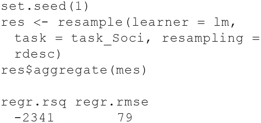
We start with a graphical demonstration based on the Titanic data set, which is simpler to interpret than examples based on the PhoneStudy data. The decision tree in Figure 5 predicts whether passengers of the Titanic survived or died in the disaster, dependent on demographic (age, sex) and voyage variables (pclass: passenger class; sibsp: number of siblings or spouses aboard; parch: number of parents or children aboard). The tree is “grown” from the root node on the top, which contains all observations in the data set. The label above each node (survived vs. died) shows the prediction we would make for each passenger belonging to this node. The numbers below the label show how many passengers died (left) and survived (right). Below each node, we see some logical criterion used to split the “parent node” into exactly two “child nodes.” Passengers are sent to the left child node if the split-condition (e.g.,
Classification tree fitted to the Titanic classification task. Passenger characteristics are used to predict whether a passenger survived the Titanic disaster. pclass = passenger class; sibsp = number of siblings or spouses aboard; parch = number of parents or children aboard. Node color encodes the classification made for the observations in that node (dark = died, light = survived).
The classification and regression trees algorithm
The tree in Figure 5 used the classification and regression trees (CART) algorithm by Breiman et al. (1984). Although many different algorithms for decision trees have been developed, the CART algorithm is still the most frequently applied one. According to which principles did the CART algorithm construct the displayed tree? Decision trees use features to iteratively partition the data space into subregions (i.e., nodes). The same prediction is computed for all observations in each node, usually on the basis of the mean (regression) or the mode (classification) of the target in that node. An optimization criterion simultaneously determines which splitting-variables and which split-points are used in the tree-growing process. The goal is to construct large nodes that contain observations with most similar target values. The similarity or purity of target values is quantified by a so-called impurity function. Intuitive impurity functions are the MSE for regression and the MMCE for classification. When regression trees make constant predictions in each node on the basis of the target mean, the MSE is equal to the observed variance of the target in a node (
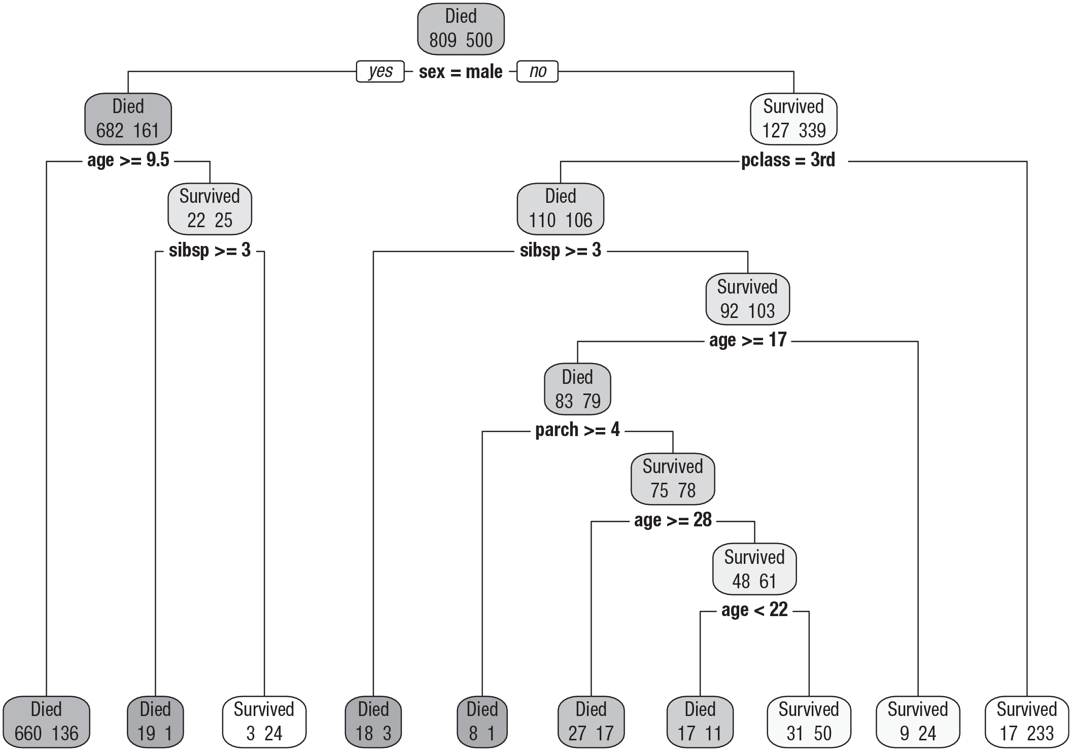
Figure 6 visualizes the tree-growing process for a regression example based on a reduced version of the AmesHousing regression task from two different perspectives. The sale price of a property is predicted with the two continuous features, Gr_Liv_Area (the above-ground living area) and Year_Built (the construction year). On the right side of each subplot, we see the already familiar tree visualization of the split-variables and split-points starting from the complete training data set on the top. On the left side, we see the corresponding prediction surface of the tree at that stage: a visualization of which target value is predicted for each combination of feature values. Each point is one property, and the true sale price is color coded (low prices in blue, high prices in red). CART trees always split the feature space into rectangles of different sizes along the feature axes. All observations falling into the same rectangle get the same target prediction (i.e., the mean sale price of all properties in that rectangle). The predicted sale price is represented by the surface color of each rectangle. In each consecutive step of the tree-growing algorithm, one rectangle is split into two smaller ones, hopefully converging toward a state in which observations in the same rectangle have roughly similar target values. The tree in Fig. 6d (with eight splits) shows the result when growing the CART tree with the default stopping criteria of the rpart R package.
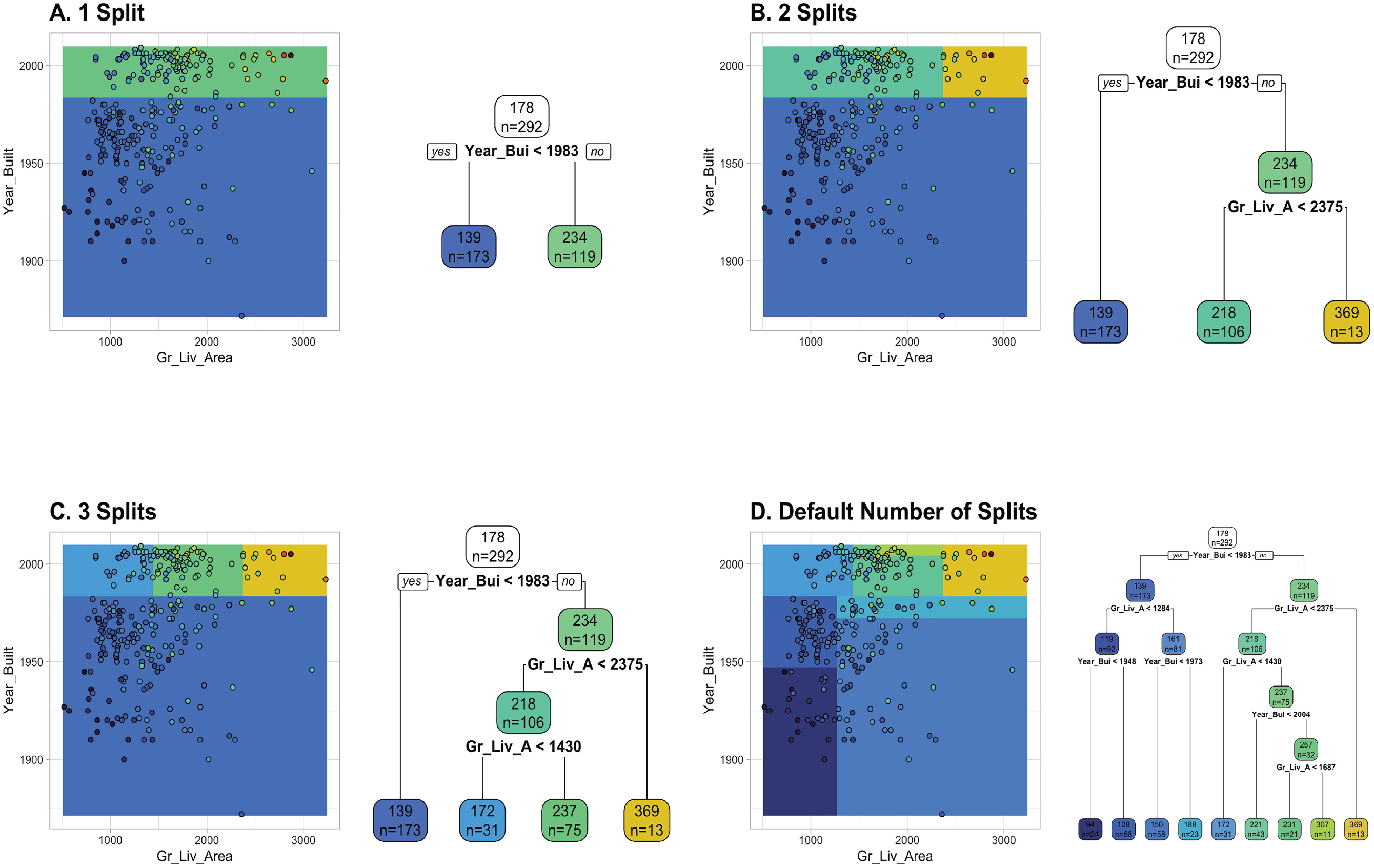
Visualization of the tree growing process by displaying the prediction surface alongside the tree structure. The plot is based on the AmesHousing regression task with two continuous features, Gr_Liv_Area (above-ground living area) and Year_Built (construction year). True and predicted sales prices of properties are color-coded (low prices in blue, high prices in red). The number of splits increases by 1 from Fig. 6a to 6c. The last plot in panel Fig. 6d shows the result of using the default stopping criteria.
Advantages and disadvantages of decision trees
Decision trees have several advantages (Hastie et al., 2009), which we briefly list here but more thoroughly demonstrate and visualize in ESM 5 (same for disadvantages): (a) Trees offer a graphical display of the predictive model, including an intuitive illustration of nonlinear interactions. It is often easier to explain a tree model than a regression model to decision makers because the tree does not require an understanding of model equations. (b) Tree models are relatively robust against outliers in the features. The algorithm depends only on the ranks in each feature and thus is also invariant against monotone transformations such as standardization. (c) Trees can model nonlinear relationships by performing several splits on the same feature in a data-driven way. The amount of splits, and thus the flexibility of the model, will automatically increase with sample size (when stopping criteria are selected with care). (d) The tree algorithm automatically performs variable selection. Uninformative features should not be selected as split variables because other features will provide higher impurity reduction. Features that are not selected as split variables during construction do not have any influence on predictions. Because of the variable selection property, trees can be effective with a possibly large number of features—uninformative features will not be selected.
However, trees also have disadvantages (Hastie et al., 2009): (a) Trees have problems modeling truly linear relationships because a large number of splits is necessary for a smooth approximation with step functions. (b) In addition, the tree structure can be highly unstable (i.e., trees trained on different samples from the same population vary a lot) if the ratio of sample size to number of features (or the general signal to noise ratio) is low. If the tree structure is unstable, this also implies that interpretations based on the structure can be unreliable. If the tree will be used for interpretation purposes, checking the stability of the model should be a high priority (Philipp et al., 2016). (c) An important hyperparameter to stabilize trees is the stopping criterion, which has a strong influence on the bias-variance trade-off of the model. Setting liberal stopping criteria (i.e., allowing many splits) will result in deeper trees that have a lower bias but also a higher variance (i.e., higher instability). Because the optimal trade-off depends on many factors, such as sample size, number of features, and the signal-to-noise ratio, elaborate tuning of stopping criteria is often required in practice. In this tuning process, a perfect trade-off between predictive performance and interpretability is difficult to achieve. The most predictive model will often be too unstable to use the tree structure for high-stakes interpretations. (d) Last but not least, although decision trees are powerful predictive models, their predictive performance (even with elaborate tuning) is often lower compared with more complex ML models.
Random forests in theory
Basic principles
Next, we introduce a procedure called “bootstrap aggregation” (Bagging; Breiman, 1996) to improve the predictive performance of decision trees by reducing variance (remember our section on the bias-variance trade-off). Variance reduction is achieved by aggregating the predictions of many trees. The Bagging algorithm (a) draws a number of bootstrap samples with replacement, (b) fits a deep decision tree (with liberal stopping criteria) on each bootstrap sample, and (c) aggregates the predictions across all trees (using the mean for regression or the mode for classification). The intuition is that the bootstrap simulates drawing multiple samples from the population of interest. Because decision trees with liberal stopping criteria have low bias but high variance, the tree structure on different (approximate) samples will vary. By averaging predictions from different trees, the low bias is retained, but the variance can be reduced, resulting in a better bias-variance trade-off and thus better predictive performance. However, one remaining limitation is that the high “correlation” between trees reduces the effectiveness of variance reduction. In this context, correlation means that (despite some instability), the tree structure on different samples shows great similarity because informative features have a high chance to be selected early in the tree-growing process. Early splits have a high influence on the tree structure and thus on the predictions made by those trees (James et al., 2021).
The RF algorithm
With the RF, Breiman (2001a), who also developed the CART algorithm and Bagging, found a clever way to improve the variance reduction from Bagging by reducing the similarity of trees in the forest: For each split, the RF algorithm draws a random subset of features that are taken into account by the optimization algorithm. At the same time, the RF uses highly liberal stopping criteria to assure minimal bias. The final RF algorithm has three major hyperparameters: (a) the number of trees to be aggregated (num.trees), (b) the number of features to consider at each split (mtry), and (c) the minimum number of observations in a node to continue splitting (min.node.size). In contrast to many other state-of-the-art ML models that require excessive tuning of hyperparameters to achieve good predictive performance, the RF typically performs well without tuning (Bernard et al., 2009; Probst et al., 2019). Useful default values are
Figure 7 visualizes how the RF predictions change with an increasing number of trees using the reduced AmesHousing regression task with two continuous features. For
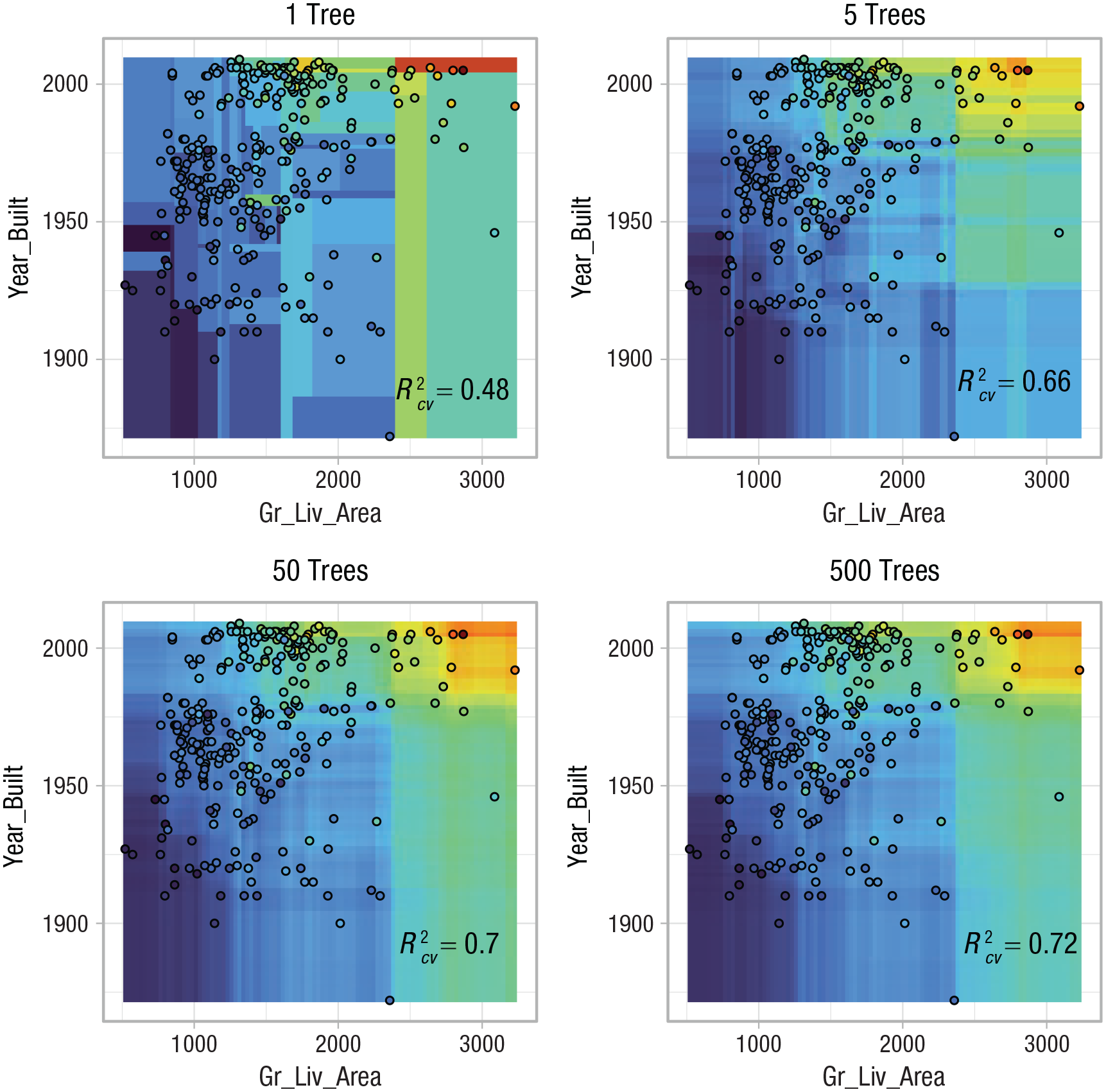
Visualization of how the smoothness of the prediction surface of a random forest changes with an increasing number of trees (from 1 to 500 trees). The plot is based on the AmesHousing regression task with two continuous features, Gr_Liv_Area (above-ground living area) and Year_Built (construction year). True and predicted sales prices of properties are color-coded (low prices in blue, high prices in red). Performance estimates are based on 10-fold cross-validation.
Advantages and disadvantages of RFs
The RF is often thought to be one of the best “off-the-shelf” models (Fernández-Delgado et al., 2014) with many advantages. Although more complex models that require excessive preprocessing or hyperparameter tuning might be able to achieve slightly better performance (e.g., XGBoost, Chen & Guestrin, 2016; deep neural networks, Goodfellow et al., 2016), the RF often reaches satisfying performance with less effort and less computational resources (i.e., models can usually be trained and evaluated on a laptop in only a few minutes). (a) The RF inherits all advantages from single decision trees (except interpretability). (b) In addition, the RF can be expected to achieve better (or at least comparable) predictive performance than single trees. All in all, the RF can be thought of as an ML model with both low bias and low variance. It keeps the low bias of deep decision trees and achieves low variance by effective variance reduction via aggregating predictions from trees with small correlations. (c) The RF handles nonlinearity and interactions even better. In contrast to linear models or single decision trees, the RF can handle even stronger nonlinear relationships between the features and the target. A visual demonstration of an artificial nonlinear classification problem is given in ESM 5.5. (d) The RF is easy to use because tuning of hyperparameters is not necessarily required. Note that there is no danger that increasing the number of trees in the RF might decrease predictive performance. Although extremely few trees will lead to suboptimal performance, the only disadvantage of an excessive number of trees is a waste of computational resources. This is in sharp contrast to other methods such as boosting (Friedman, 2001), which will strongly overfit to the training data if the number of trees is not tuned carefully (James et al., 2021).
Of course, the RF also has a few disadvantages: (a) The RF might still not be ideal for truly linear relationships, although a sufficiently large number of trees can approximate smooth functions much better than a single tree. (b) Possibly the biggest disadvantage is that the RF loses the convenient interpretability of single trees. It is not useful to inspect graphical displays of hundreds of trees that are aggregated for the final predictive model. Additional tools from the field of interpretable ML are necessary to interpret RF predictions. We introduce such methods later.
Practical Exercise 2: train an RF and estimate predictive performance
In the next exercise, we show how to train and evaluate a RF model in mlr3. We use a classification problem in this exercise to demonstrate how classification is done in mlr3. However, the RF also works for regression problems, which we demonstrate in the next module. To follow along, make sure to repeat the earlier code steps in which we loaded the PhoneStudy data set.
Create a classification task
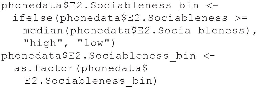
First, we create an artificial classification example by binning the continuous E2.Sociableness variable into “high” and “low” sociability according to the median of the complete data set. This is just to showcase how classification works in mlr3. We do not recommend binning in a real application, in which we would always perform regression if the target is continuous (Stachl, Pargent, et al., 2020):
We create a new supervised classification task on the basis of the binned target, declaring high sociability as the so-called positive group. This arbitrary choice determines the interpretation of performance measures such as
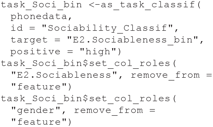
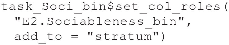
In the following line, we specify our target as a so-called stratification variable. When we later split the task for CV, this will (roughly) keep the proportion of high and low sociability in each training set equal to the proportion in the complete data set. Using stratified resampling for classification tasks is usually a good idea because it improves the precision of performance estimates, especially for data sets with imbalanced classes or relatively few observations (Kohavi, 1995):
Train a random forest model
Next, we create a learner for the RF model, using the state-of-the-art implementation in the ranger package (Wright & Ziegler, 2017). We can directly specify hyperparameter settings of the learner (e.g., the number of trees). To handle the missing data, we again fuse our learner with our imputation strategy and create a GraphLearner. Because the RF algorithm contains random steps (drawing bootstrap samples), we set a seed before training the learner on our classification task to make the results reproducible.
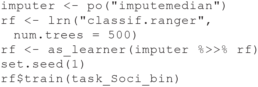
The trained model object produced by the ranger package could be extracted with
As before, we could also calculate in-sample predictive performance by computing predictions for the same data used in training. Now that we have a classification task, the prediction object also contains a confusion matrix of our in-sample predictions:
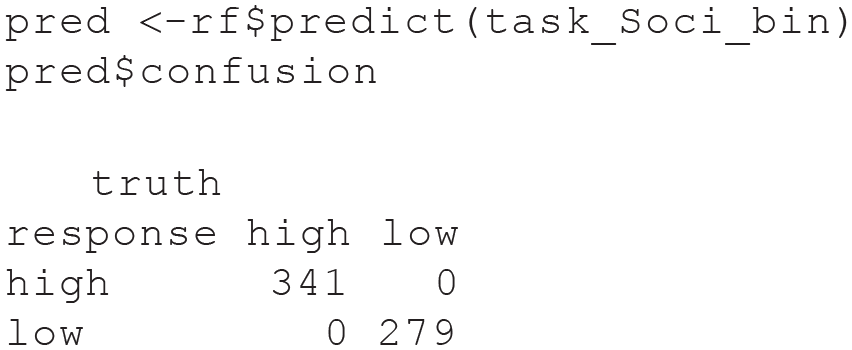
All observations from the training data have been classified without error. However, this estimate is probably not realistic for the predictive performance on new data.
Estimate predictive performance of the model
The following out-of-sample estimate exemplifies again that in-sample performance estimates should not be trusted, especially not for flexible ML models such as RF. It is absolutely necessary to use resampling, here 10-fold CV with
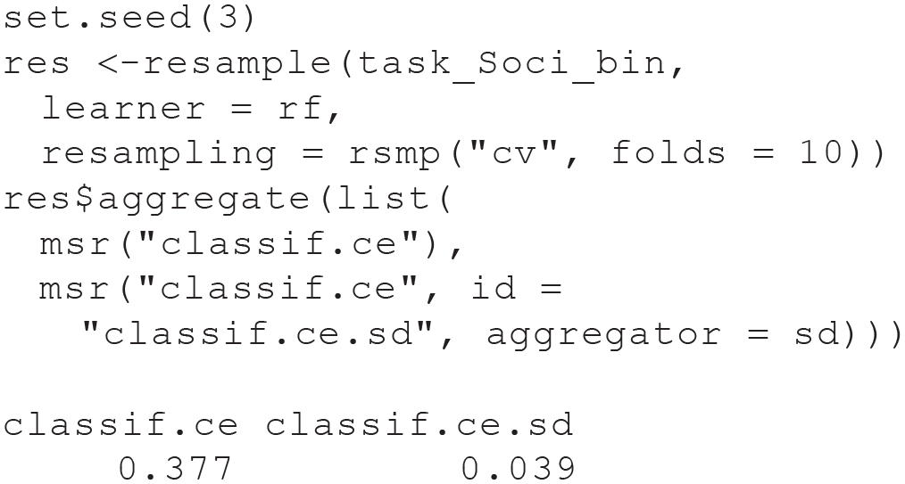
CV reveals that the full model cannot be expected to perfectly predict new data but will misclassify about 38% of all cases. Note that we computed both the already familiar point estimate of predictive performance (mean
Summary of Module 2
In Module 2, we introduced the RF, a popular nonlinear ML model with strong predictive performance and high usability. The logic of the RF is quite different from the linear regression models that psychologists are most familiar with: The RF algorithm averages the predictions from a large number of decision trees that are grown with the CART algorithm. We took our time to explain those important underlying concepts with graphical illustrations. In Practical Exercise 2, readers were guided on how to train and to evaluate the predictive performance of an RF model with mlr3, thereby rehearsing important concepts introduced in Module 1.
Module 3: Benchmark Experiments
Model comparisons as controlled scientific experiments
When performing supervised ML in practice, it is often necessary to compare predictive performance estimates for different types of models because there are no effective heuristics on which models are optimal under different settings. These so-called benchmark experiments include an assessment of whether a model has superior predictive performance in comparison with a baseline or state-of-the art model. Often a “featureless” learner is used as a simple baseline model against which the performance of the other models of interest are compared. The featureless learner uses the mean target value in the training set as a constant prediction for all observation in the test set, thereby effectively ignoring the information from all features. Useful ML models should be able to at least beat the featureless model. Even stronger theoretical baseline models can be designed for most applications (e.g., predict personality scores on the basis of only demographic variables). Benchmarks strongly resemble scientific experiments or randomized controlled trials; they investigate the effect of choosing a predictive model on the expected predicted performance: Different experimental conditions or treatments (i.e., types of models) are compared with a control group (i.e., featureless learner). For each experimental condition, the optimal stimulus intensity or “dosage” is identified and applied (i.e., nested tuning of all hyperparameter settings). To ensure fair comparisons, external factors (i.e., performance measures, resampling strategies including the concrete assignment of observations to training and test sets) are kept constant between conditions.
Practical Exercise 3: model comparisons with benchmark experiments
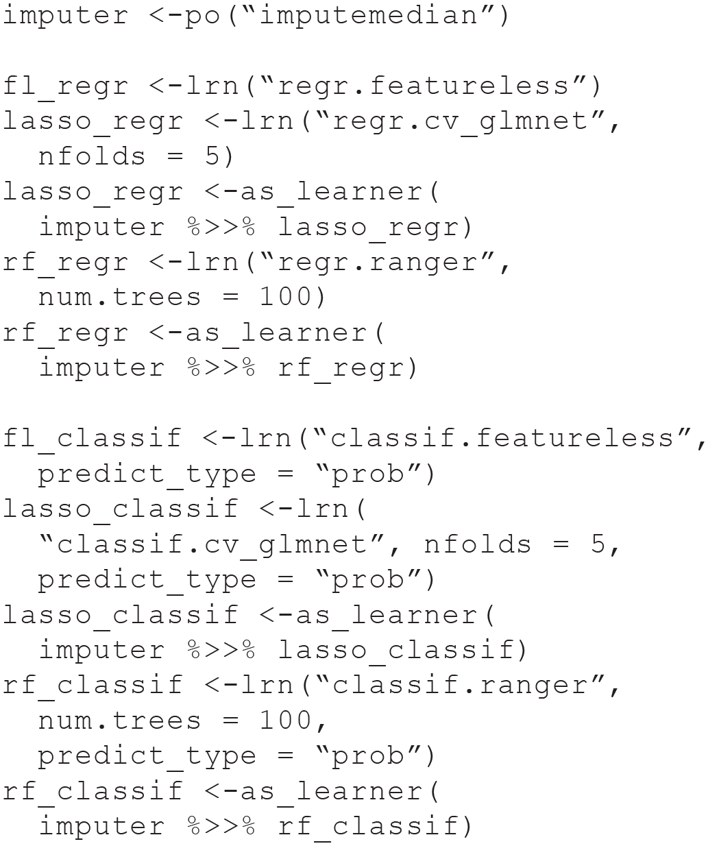
In our third exercise, we conduct two benchmark experiments. The first benchmark experiment illustrates a regression task, the second a classification task. We apply the RF from Module 2, along with other learners. Besides a featureless learner, we also compare the RF to a so-called least absolute shrinkage and selection operator (LASSO) model (Tibshirani, 1996) in our benchmark experiments. The LASSO is a linear regression (or classification) model that can effectively include a large number of features by shrinking the coefficients toward zero. This shrinkage also results in coefficients of exactly zero for unimportant features, thereby performing automatic variable selection because the corresponding features will not be taken into account when computing predictions. The results can be interpreted similar to ordinary linear or logistic regression because the LASSO can be seen as an alternative method to estimate the model parameters of these models. We have observed in our own ML applications that LASSO often performs comparably or even better than RF on survey data (e.g., Pargent & Albert-Von Der Gönna, 2018). Thus, we recommend by default to include the LASSO into benchmark experiments when working with psychological data. A nontechnical introduction to the LASSO was provided by James et al. (2021).
For our benchmark analysis, we reuse the task_Soci and task_Soci_bin objects we created earlier. We create GraphLearners fused with imputation (featureless learner, LASSO, and RF) for both a regression and a classification task. The featureless learner does not require imputation because it does not use any features: 10
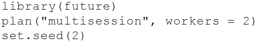
Because benchmark experiments easily become computationally intensive, we use parallelization (speeding up computations by using more than one core of the computer simultaneously), which is provided by the future package (Bengtsson, 2021). To use parallelization with mlr3, the only steps are to load the future package, specify a parallelization plan (use
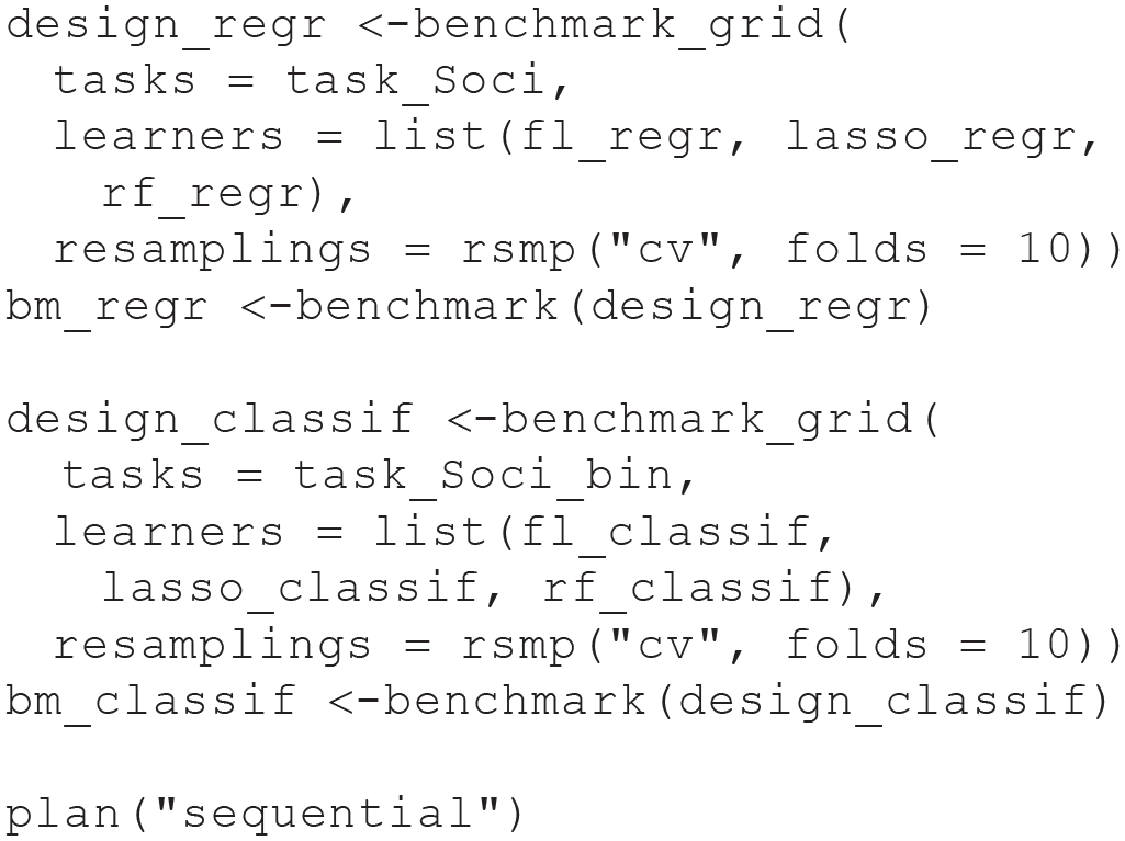
Before we can actually compute the individual benchmark experiments for our regression and classification tasks, we have to declare our benchmark designs. These designs specify which learners will be trained on which tasks and which resampling strategies should be used for each combination of Learner × Task interaction. We choose 10-fold CV to enable computation on smaller laptops in a reasonable amount of time for our tutorial. In a real application, we would apply repeated CV here because performance estimates have a high variability for this example (notice how the estimates change when repeating the benchmark with different seeds). After running the experiments by calling the
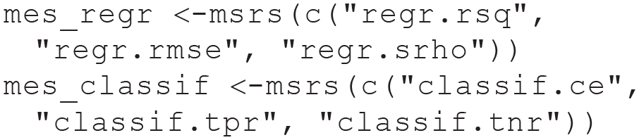
We choose an extended set of performance measures for our regression and classification benchmarks. For regression, we look at
First, we compute aggregated performance for the regression benchmark with
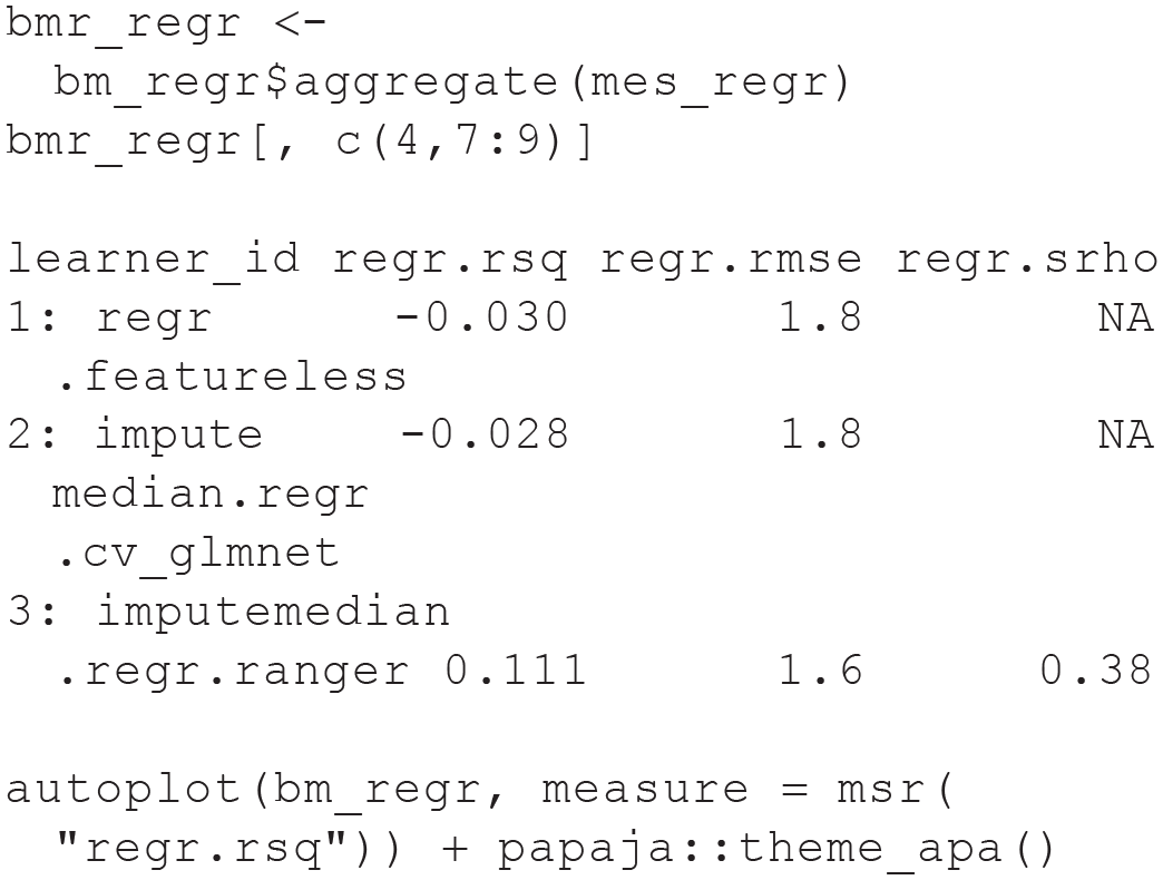
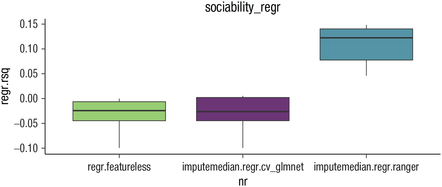
Box plots displaying the results of the benchmark experiment of the Sociability regression task using the PhoneStudy data set.
It seems that the RF produces more accurate predictions than the LASSO and the featureless learner for all performance measures. Note that the Spearman’s correlation could not be computed for the LASSO and the featureless learner because both produced constant predictions for all observations in at least one fold. Although this must always be the case for the featureless learner (i.e., constant prediction based on the target mean in the training set), it seems that the LASSO automatically removed all features from the model (i.e., constant prediction based on the model intercept). This observation reflects the bad performance of the LASSO, which cannot effectively use the information contained in the features in this example.
The commands to display benchmark results are similar for the classification benchmark. Instead of the grouped box plot, we here show how to produce a simple ROC plot (see Fig. 9) by calling
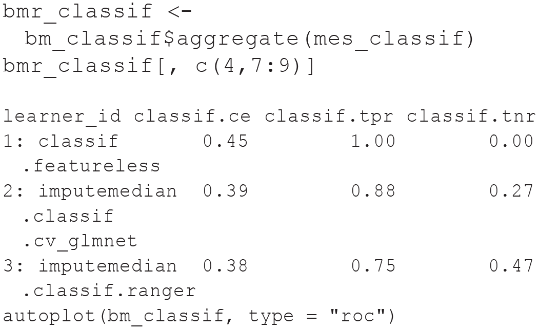
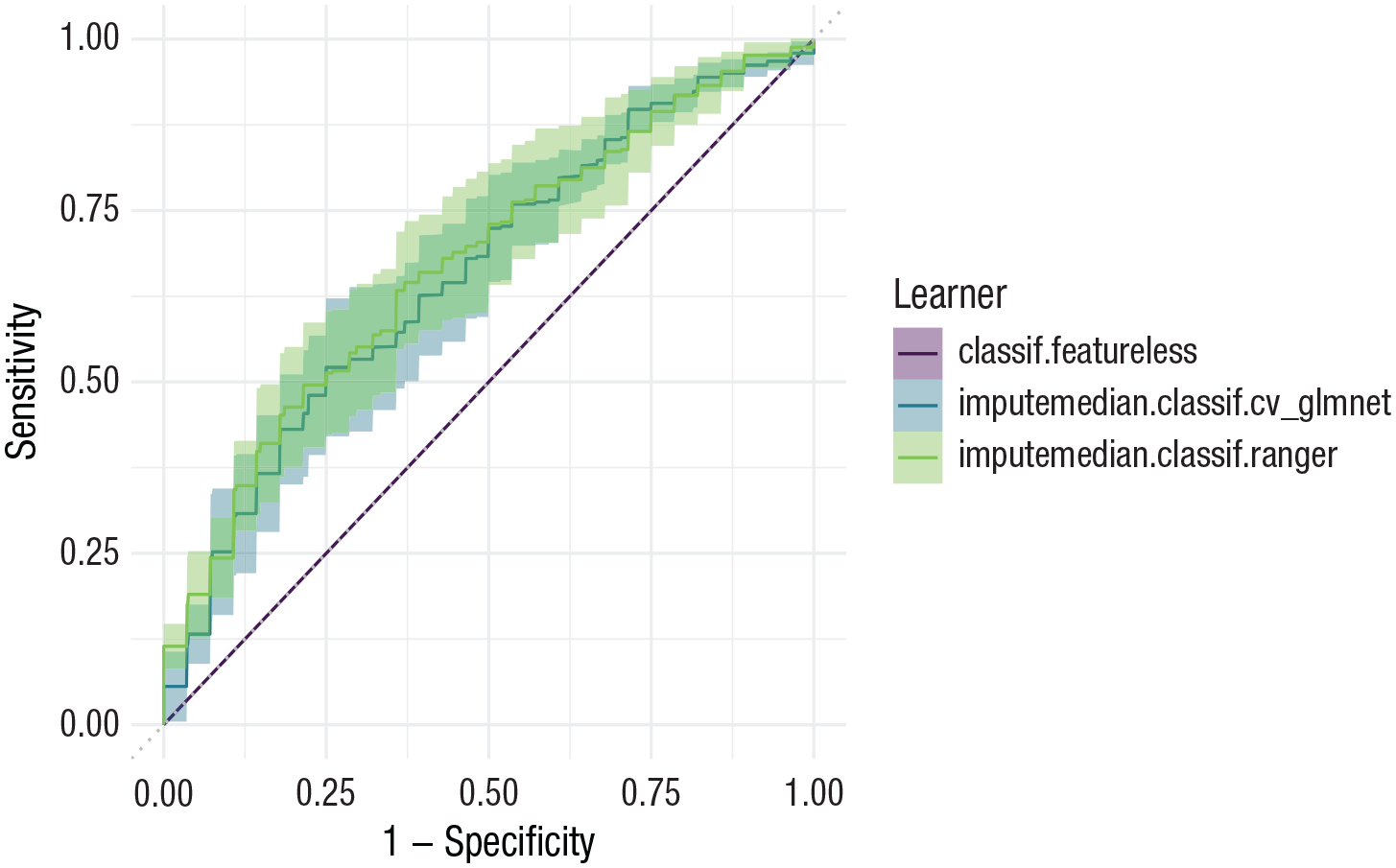
Receiver operating curve
When looking at the results, we notice that although
To practice with another benchmark example, ESM 6 contains mlr3 code to perform a benchmark experiment with the Titanic data set.
Summary of Module 3
Module 3 introduced benchmark experiments. Supervised ML usually requires comparing the predictive performance of different types of ML models because researchers cannot know in advance which model will perform best for the specific research question at hand. This comparison typically includes a featureless baseline model to answer the question whether a predictive model performs better than naive guessing. Practical Exercise 3 took readers step-by-step through the process of setting up benchmark experiments in mlr3, which draws on the skills obtained in Module 1 (i.e., performance evaluation via resampling) and Module 2 (i.e., training an RF). We demonstrated how to interpret benchmark results and highlighted the importance of different performance measures and the variability of performance estimates.
Module 4: Interpretation of Models
Interpretable ML
In addition to training models for practical applications or answering substantial research questions on the basis of benchmark experiments (Rocca & Yarkoni, 2021; Shmueli, 2010; Yarkoni & Westfall, 2017), researchers often want to understand how the final model makes predictions to connect findings to psychological theories. Understanding model predictions is the goal of interpretable ML (IML; Molnar et al., 2020). We focus solely on model-agnostic methods that can be applied with any trained predictive model and are not limited to a specific type of ML model (e.g., RF). We do not discuss a contrasting view that focuses on building inherently interpretable models (e.g., simple decision rules) instead of explaining the predictions from black-box ML models (Rudin et al., 2022).
Many IML methods can be broadly categorized to answer one of two important questions. First, which features have the biggest effect on model predictions? This question can be answered with variable importance measures. Second, how do individual features influence model predictions? This question can be answered with effect plots. We briefly describe these methods in the following sections. For an extensive introduction to IML methods for psychological research, see Henninger et al. (2022).
Variable importance measures
Variable importance measures try to answer the following question: Which features are most influential for model predictions? They are mostly inspired by the RF (Breiman, 2001a) but were extended to work with arbitrary ML models. We focus on the model-agnostic permutation variable importance (PVI; Fisher et al., 2019). PVI formalizes the intuitive idea that a model should make a bad prediction for an observation if the data for this observation contain an accidental mistake in an important feature (e.g., a young age was recorded for an old person). PVI takes a set of observations and shuffles the observed values in the feature of interest (e.g., persons are randomly assigned the age values of other persons in the sample). This permutation destroys the systematic information in the feature, which could be used to meaningfully predict the target. Predictions are computed for all observations with the shuffled feature values, and the actually observed values are used on all remaining features. Note that the model that is used to compute predictions is always trained on the unshuffled data. Predictive performance is calculated under the shuffled condition and compared with the performance under the normal condition with unshuffled values. The greater the performance difference, the more important the respective feature is (e.g., if age is an important feature, predictive performance should suffer when the observed age values are assigned to the wrong persons). In contrast, if a feature is not important (i.e., unrelated to the target), shuffling should not decrease predictive performance. By repeating the process for each feature, PVI produces a ranking of important features. The resulting PVI values should be interpreted only in comparison with each other because the absolute values are difficult to interpret. In principle, PVI automatically captures both main and interaction effects. However, it does not say anything about the direction of the effect, the shape of the effects, or whether an important feature has any causal effect on the target.
Figure 10a shows the PVI rankings for the Titanic task. Because this is a classification task,

A visualization of interpretable machine-learning methods applied to a random forest model trained on the complete Titanic data set. (a) The permutation variable importance for each feature. (b) Effect plot of the age feature, combining the individual conditional expectation profiles (gray lines) with the partial dependence (blue line). pclass = passenger class; sibsp = number of siblings or spouses aboard; parch = number of parents or children aboard.
Standard PVI has been known to overestimate the importance of features with many unique values (Strobl et al., 2007) or high correlations with truly important features (Strobl et al., 2008). Unbiased PVI measures have been developed, but they are not model-agnostic and work together only with a specific RF algorithm based on recursive partitioning (Debeer & Strobl, 2020; Strobl et al., 2008). Unfortunately, this newer RF version is less computationally efficient and requires more extensive hyperparameter tuning to perform well, which is why we do not use it as a default. For a short discussion on RF-specific variable importance measures, see ESM 7.1.
Effect plots
Effect plots try to answer the following question: How do individual features influence model predictions? Effect plots display how model predictions change for different values of some feature of interest. Like in PVI, this is done by substituting the actual feature values, but now values are changed systematically instead of randomly. A prediction for an individual naturally uses the actually observed value in a feature of interest (e.g., a person is 40 years of age). However, the trained model could also compute a prediction for a different feature value (e.g., “pretending” that the observed age for this person is 60). In this way, a range of predictions can be computed for each individual by systematically changing the values in the feature of interest (e.g., on a grid of age values between 0 and 80 years) while keeping the actually observed values on all other features. Visualizing these profiles for a group of observations is called an “individual conditional expectation” (ICE; Goldstein et al., 2015) plot.
Figure 10b shows the ICE plot for the age feature in the Titanic task. Each line shows predictions for a single person computed with different age values (shown on the x-axis), and the points mark the actually observed age value for each person. ICE profiles can sometimes reveal interactions of the feature of interest with other, potentially unknown variables. For example, there seems to be a group of persons (the lines on the top) for which the predicted probability of surviving (shown on the y-axis) does not change with different age values. This seems in contrast to another group of persons (the lines in the middle) for which predicted survival probabilities decrease with higher age values. These different shapes indicate an interaction of age with one or several other features, which might be either contained in the data set or completely unobserved. For further exploration, one could color the lines on the basis of a feature suspected to be responsible for these interaction (e.g., pclass or sex) and see whether systematic patterns emerge.
ICE plots can be a bit overwhelming, and a more simple summary might be desired. The thick line in Figure 10b shows the average profile by vertically computing the mean across all lines for each feature value on the x-axis. If this average is displayed without the individual profiles, the resulting curve is called a “partial dependence” (PD; Friedman, 2001) plot. The PD in our example indicates that on average, the predicted survival probability decreases for higher age values. However, keep in mind that the ICE profiles show that this average trend is not observed for all persons. Note also that effect plots do not necessarily indicate that the feature of interest has any causal effect on the target.
An alternative to PD are “accumulated local effects” (ALEs; Apley & Zhu, 2020) plots. Although ALEs plots are often discussed as an improvement on PD, this does not seem to be without controversy because both estimate slightly different concepts. Molnar (2019) and Henninger et al. (2022) provided a clear introduction on both methods.
Model fairness
Closely related to IML is the topic of model fairness (Barocas et al., 2019). Intuitively, a trained ML model is considered fair if it does not discriminate against protected subgroups of observations (e.g., gender groups; Buolamwini & Gebru, 2018). However, which specific model behavior is considered fair is highly context-specific because it entails some normative consensus. It has been argued that all ML models applied in practice should be accompanied by transparent documentation on their performance characteristics and their intended use cases (Mitchell et al., 2019). Fairness seems particularly relevant when ML is used in psychological assessment (Stachl, Pargent, et al., 2020). In such settings, the “protected attribute” (e.g., the gender variable in the data set) is usually not included as a feature in the model to prevent the model from using the information in the protected variable to predict the target. However, flexible ML models often implicitly infer group membership on the basis of available features that are related to the protected attribute. Thus, it is necessary to explicitly evaluate fairness by comparing predictions for observations with different values on the protected attribute. Many techniques introduced in our performance evaluation and IML sections can be useful to creatively explore whether a trained model behaves as required by a fairness definition appropriate for the concrete use-case of the model. We give brief examples of two different fairness aspects in our applied section and refer readers to Barocas et al. (2019) for an extensive overview of fairness definitions and evaluation strategies. First, is the predictive performance of the model comparable for different values of the protected attribute? This can be evaluated by estimating out-of-sample performance separately for each value of the protected attribute. Second, do model predictions differentially depend on the value of some feature of interest for different values of the protected attribute? This can be evaluated by computing PVI rankings or ICE/PD plots separately for each value of the protected attribute.
Comments on causal interpretation
Most methods introduced in the IML and fairness sections seem to have an intuitive interpretation. However, we point out that it is of utmost importance not to carelessly interpret the results in a causal manner. Generally, those methods investigate only the relationship between feature values and model predictions. They do not necessarily reflect the true data-generating process (Zhao & Hastie, 2021). It is a well-known fact in the causal-inference literature that causal claims always rely on strong assumptions that cannot be fully inferred from the observed data itself (Pearl, 2009). A common definition for a causal effect of some feature on the target is that a (hypothetical) intervention on the feature would lead to a different target value. Even if some ML model accurately estimated the correlation structure between the target and the features, this does not necessarily mean that features with high PVI are good candidates to focus in interventions if the aim is to influence the true target values. In addition, PD and ICE plots do not show how the true target values would change if some intervention could achieve specific values on the feature of interest without intervening on the other features. Similar arguments are true for fairness aspects (Plecko & Bareinboim, 2022). Without a causal model, one cannot differentiate between a situation in which a model directly discriminates against certain values of a protected attribute (e.g., women earn less money because they are women) versus indirectly (e.g., women earn less because they choose professions with lower income).
Recent calls in psychology urge to take questions of causal inference seriously, and intuitive tutorials on choosing the right control variables in statistical modeling are now available (Deffner et al., 2022; Rohrer, 2018; Wysocki et al., 2022). IML methods are no magical devices that justify ignoring these considerations. Zhao and Hastie (2021) explained under which assumptions PD and ICE plots may be interpreted as causal effects. A causal perspective on ML fairness is given in Plecko and Bareinboim (2022). We strongly advise all readers to deeply think about whether the results of IML and fairness analyses will actually be useful to serve the intended purpose in their specific case. There might be many circumstances in which such reflections will reveal that explicitly modeling the causal mechanisms is necessary to ensure that predictions will be practically useful.
Practical Exercise 4: IML with mlr3 and DALEX
For our empirical demonstration, we use the DALEX/DALEXtra R packages (Biecek, 2018), which come with a detailed online textbook (Biecek & Burzykowski, 2021). An alternative is the iml package (Molnar et al., 2018), with its excellent online companion book (Molnar, 2019). The mlr3 e-book also contains a chapter on how to use both frameworks (Bischl et al., 2023). We use all IML methods on an RF model trained on the complete Sociability regression task. For a discussion on whether using IML on the complete data set or using some combination of training and test sets, see Chapter 8.5.2 in Molnar (2019).
First, we train the RF GraphLearner from earlier (which includes the imputation pipeline) on our complete Sociability task:
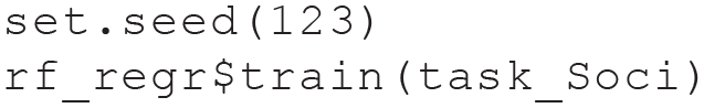
Then we construct an “explainer” object from the DALEXtra package, which takes the following as main inputs:
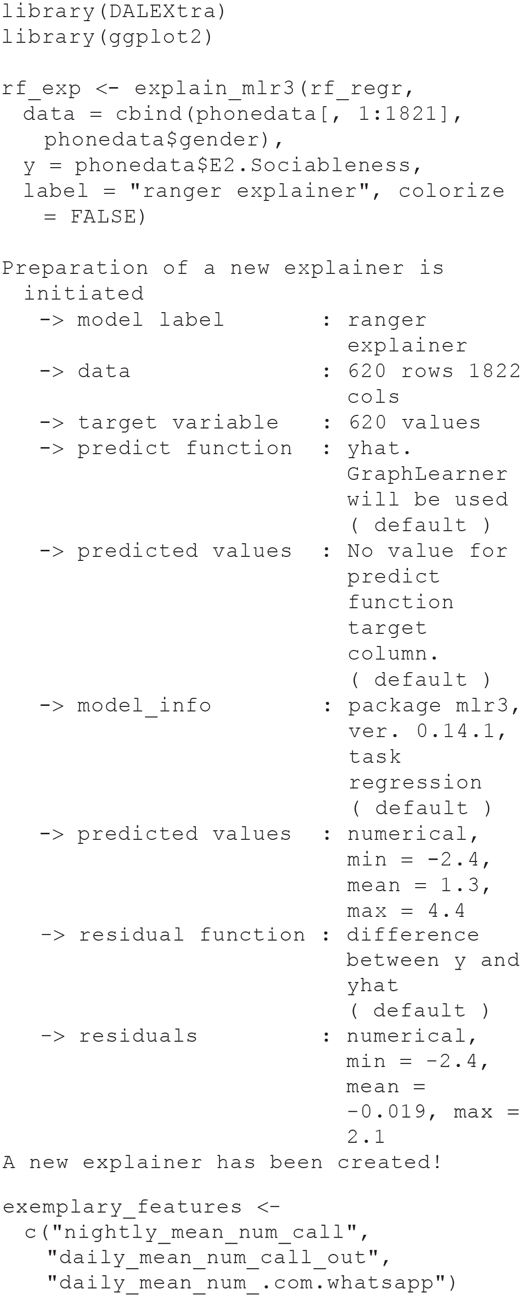
The explainer object can be used for all IML methods included in the DALEX/DALEXtra packages. To reduce the computational load for this tutorial, we use only a small subset of exemplary features for which we compute the IML methods. In practice, we would include all features from our task.
Permutation variable importance
To compute PVI, we use the
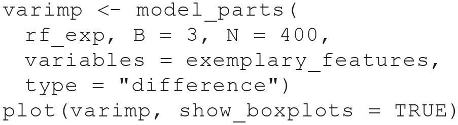
We use only a subset of observations (

Permutation variable importance for three exemplary features based on the random forest model trained on the full Sociability regression task.
The PhoneStudy data set consists of a very large number of features. In such settings, it can be more enlightening to interpret variable importance for groups of features (e.g., app categories; see Stachl, Au, et al., 2020). 12
ICE profiles and PD plot
The
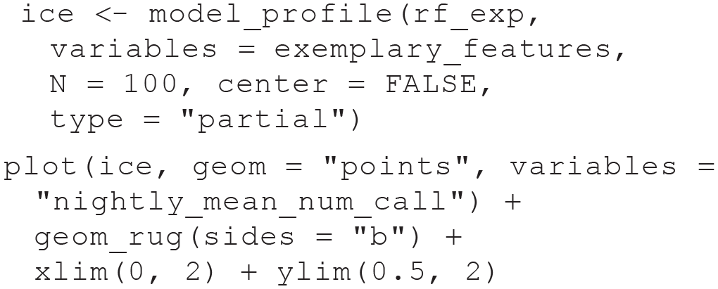
Each ICE profile (i.e., each line in the plot) in Figure 12 corresponds to one person in our data set. It shows how the model’s predicted sociability for this person (on the y-axis) changes when we arbitrarily set the average number of telephone calls at night (nightly_mean_num_call; on the x-axis) to different values across the observed range while keeping the person’s observed values on all other features. In this example, there is no sign for any strong interactions, and the effect of all single features on the target seems quite weak (nightly_mean_num_call is already the most important feature measured by PVI; see Stachl, Au, et al., 2020). The PD is already displayed in the ICE plot in Figure 12 as the bold blue line. We could also request the PD by itself with

Individual conditional expectation profiles for the average number of telephone calls at night (nightly_mean_num_call) based on the random forest model trained on the full Sociability regression task.
Note that for these PhoneStudy examples, IML methods do not reveal causal effects: Personality theory would consider it unreasonable that some intervention that would simply call study participants at late hours, thereby increasing the average number of telephone calls at night (feature nightly_mean_num_call), would lead to an increase in those participants’ sociability.
Aspects of model fairness
To explore whether the predictive performance of our model differs between men and women, we compute predictive performance separately for each gender with the mlr3fairness companion package (Pfisterer et al., 2022). When mlr3fairness is loaded before creating task_Soci, we can declare gender as a protected attribute (pta). We can then create groupwise performance measures that automatically take this variable into account:
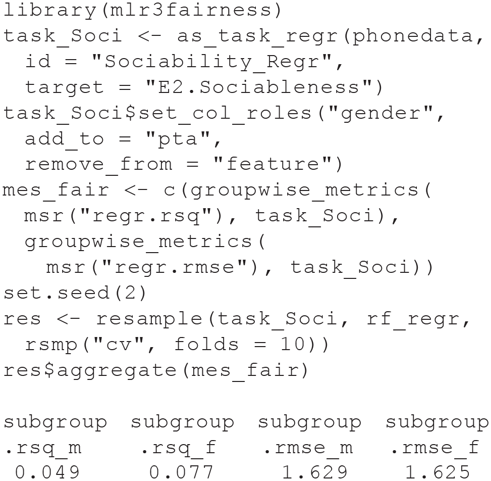
The resampling results suggest that our model makes more accurate predictions for women (f) than for men (m). One plausible reason could be that the data set contains more observations from women (61% women). The mlr3fairness package includes many more options for classification than for regression settings. Apart from evaluating fairness with different fairness metrics, it also contains methods to construct models with better fairness properties by using augmented ML models or debiasing methods.
To explore whether predicted sociability differentially depends on the value of the feature nightly_mean_num_call for men and women, the PD plot introduced earlier can be computed simultaneously for both genders, which we demonstrate in ESM 7.3. Although the form of the relationship between the feature and the target predictions seems similar for both genders, the model generally predicts higher sociability for women than for men. Note that for both fairness analyses, the gender variable was not used as a feature when training the predictive model.
Summary of Module 4
In the final Module 4, we introduced popular tools to interpret a trained predictive model. In a first step, variable importance measures can detect the features with the greatest impact on predictive performance. In a second step, effect plots can reveal the functional relationship between the important features and the target. In Practical Exercise 4, we showed how to use the DALEX R package to interpret models trained with mlr3. To prevent the practical application of models that discriminate against certain groups, in Module 4, we also gave a primer on how to evaluate model fairness. Finally, we discussed important limitations of interpretable ML and fairness methods with respect to causal inference.
Conclusion
In this tutorial, we gave an intuitive but thorough introduction to the fundamentals of supervised ML for students, researchers, and educators in psychology. After introducing important terminology and the predictive mindset of supervised ML, in Module 1, we covered the important topic of how to evaluate the predictive performance of ML models with resampling methods such as 10-fold CV. Module 2 introduced the RF, a versatile nonlinear model that serves as a useful entry point into the diverse world of ML algorithms. In Module 3, we focused on benchmark experiments, which are a structured approach to compare the predictive performance of different models and to determine which model performs better in a specific application. Finally, Module 4 discussed permutation variable importance and effect plots to interpret ML models, which is important whenever predictive performance is not the only goal to use predictive models in psychological applications. For a quick reminder on the most important considerations and common pitfalls when performing, reporting, or reviewing ML models in psychological research, we provide a convenient one-page checklist in Figure 13. The excellent textbook by James et al. (2021) that we have referenced throughout this article is an ideal starting point to read more about basic ML concepts and methods.

The checklist on the left summarizes the most important machine-learning (ML) procedures, which were presented in detail in our tutorial. These reminders are intended for readers when performing, reporting, or reviewing ML analyses. The list of lessons learned on the right summarizes some of the authors’ own subjective experiences when running analyses and reviewing ML articles. In combination, they might save our readers from some of the most common pitfalls and surprises when applying ML methods in psychological research.
Our tutorial did not cover the following advanced topics, which we briefly mention for interested readers. First, the psychological community has started to construct ML models that explicitly address one important characteristic of most psychological data—measurement error (e.g., Brandmaier et al., 2013; Jacobucci et al., 2016; Jacobucci & Grimm, 2020). Second, we have not discussed some open issues of ML with latent variables but refer the interested reader to Stachl, Pargent, et al. (2020). Finally, users in psychology and other social sciences need to be acutely aware of the ethical implications that can arise from the reflected use of ML methods in applications (Mitchell et al., 2019). We gave a short introduction on the idea of model fairness, an important framework to ethically evaluate predictive models. However, additional aspects (e.g., transparency, justice, nonmaleficence) should be taken into account (Jobin et al., 2019), and psychologists must be careful not to prematurely neglect important issues of causality when focusing on prediction (Plecko & Bareinboim, 2022; Zhao & Hastie, 2021). There is also a growing literature with specific guidelines for clinical predictive models (Moons et al., 2015; Wolff et al., 2019), which require especially high methodological and ethical standards.
Supervised ML is poised to become an important method in the toolbox of psychologists, and we hope that our tutorial can help them to apply ML responsibly. Although ML is not a silver bullet to solve the generalizability crisis (Yarkoni, 2022) of our discipline, we are convinced that psychology can profit from investigating predictive research questions with ML tools, which were specifically designed to make predictive claims (Yarkoni & Westfall, 2017).
Footnotes
Acknowledgements
We thank Bernd Bischl and the mlr3 team for developing amazing open-source software and for teaching us how to perform responsible machine-learning analyses. We thank Sanaz Talaifar, Samuel D. Gosling, Meike Zehnle, and Fotis Efthymiou for valuable feedback on earlier versions of this article. We thank Anja Betz for increasing the reproducibility of our article. The first version of the article was based on a workshop we have given to various audiences in psychology and other social sciences. We thank our students and workshop participants for continuous feedback on our educational materials.
Transparency
Action Editor: David A. Sbarra
Editor: David A. Sbarra
Author Contribution(s)