Sage Journals: Discover world-class research

Abstract

An increasingly popular approach to statistical inference is to focus on the estimation of effect size. Yet this approach is implicitly based on the assumption that there is an effect while ignoring the null hypothesis that the effect is absent. We demonstrate how this common null-hypothesis neglect may result in effect size estimates that are overly optimistic. As an alternative to the current approach, a spike-and-slab model explicitly incorporates the plausibility of the null hypothesis into the estimation process. We illustrate the implications of this approach and provide an empirical example.

Keywords

effect size Bayesian estimation modeling shrinkage open materials

Consider the following hypothetical scenario: A colleague from the biology department has just conducted an experiment and approaches you for statistical advice. The analysis yields p < .05, and your colleague believes that this is grounds to reject the null hypothesis. In line with recommendations both old (e.g., Grant, 1962; Loftus, 1996) and new (e.g., Cumming, 2014; Harrington et al., 2019), you convince your colleague that it is better to replace the p value with a point estimate of effect size and a 95% confidence interval (CI; but see Morey et al., 2016). You also manage to convince your colleague to plot the data (see Fig. 1). Mindful of the reporting guidelines of the Psychonomic Society¹ and Psychological Science,² your colleague reports the result as follows: “Cohen’s d = 0.30, 95% CI = [0.02, 0.58].”

Fig. 1.

Standard estimation results for the fictitious plant growth example. (Left) A descriptives plot with the mean and 95% confidence interval of plant growth in the two conditions. (Right) Point estimate and 95% confidence interval for Cohen’s $d .$

Given these results, what would be a reasonable point estimate of effect size? A straightforward and intuitive answer is “0.30.” However, your colleague now informs you of the hypothesis that the experiment was designed to assess: “Plants grow faster when you talk to them.”³ Suddenly, a population effect size of zero appears eminently plausible. Any observed difference may merely be due to the inevitable sampling variability.

The example above is rhetorical but serves to underscore the potential conflict between standard reporting guidelines and common sense. The example raises the following question: When are effect sizes overestimated? Standard point estimates and confidence intervals ignore the possibility that the effect is spurious (i.e., the null hypothesis, $ℋ_{0}$ ). This is not problematic when $ℋ_{0}$ is deeply implausible, either because $ℋ_{0}$ was highly unlikely a priori or because the data decisively undercut $ℋ_{0}$ . But when the data fail to undercut $ℋ_{0}$ or when $ℋ_{0}$ is highly likely a priori (i.e., “plants do not grow faster when you talk to them”), then $ℋ_{0}$ is not ruled out as a plausible account of the data. Effect size estimates that ignore a plausible $ℋ_{0}$ are generally overly optimistic and overly confident: The fact that $ℋ_{0}$ provides an acceptable account of the data should shrink effect size estimates toward zero. The statistical benefits of shrinkage are described in Efron and Morris (1977; see also Davis-Stober et al., 2018; Rouder & Lu, 2005; Shiffrin et al., 2008); the benefits of shrinking estimates toward zero are discussed, for instance, in George and McCulloch (1993), Iverson et al. (2010), and van Erp et al. (2019).

The above point estimate, 0.30, may seem purely data-driven, but it is based on a model that assumes an effect size different from zero. In this article, we propose an alternative model to estimate effect size: the so-called spike-and-slab model. First, we formally introduce the spike-and-slab model. Second, we apply the spike-and-slab model to the example in the introduction and illustrate how it tempers the estimated effect size. Third, we visualize how the spike-and-slab model may shrink the estimated effect size toward zero in general. Fourth, we demonstrate the spike-and-slab model by reanalyzing the data of Heycke et al. (2018). Finally, we conclude with practical recommendations and a discussion on when to use the spike-and-slab model.

A Spike-and-Slab Perspective

The spike-and-slab approach has been widely discussed in the statistical literature (e.g., Clyde et al., 1996; Geweke, 1996; Ishwaran & Rao, 2005; Mitchell & Beauchamp, 1988; O’Hara & Sillanpää, 2009) and in the psychological literature (e.g., Bainter et al., 2020; Iverson et al., 2010; Rouder et al., 2018; Yu et al., 2018). Conceptually, the approach is relatively straightforward.

As usual, the statistical goal is to infer the population effect size from a set of sample observations. Let $δ$ denote the population effect size, let $\hat{δ}$ denote a point estimate, and let $\hat{δ} | ℋ_{1}$ denote a point estimate assuming the alternative hypothesis, $ℋ_{1}$ . Assuming the null hypothesis $ℋ_{0}$ leads to $\hat{δ} | ℋ_{0}$ , this usually equals 0. Key is that both estimates, $\hat{δ} | ℋ_{1}$ and $\hat{δ} | ℋ_{0}$ , are conditional on the hypotheses. For example, $\hat{δ} | ℋ_{1}$ should be read as “the estimated effect size under the alternative hypothesis that the effect exists.” To the best of our knowledge, all existing guidelines for reporting effect size estimates recommend that researchers provide $\hat{δ} | ℋ_{1}$ ; implicitly, the guidelines suggest to ignore $ℋ_{0}$ , resulting in the notion that the population effect size is nonzero. In contrast, in the spike-and-slab model, the estimate of effect size is determined by both $ℋ_{1}$ and $ℋ_{0}$ .

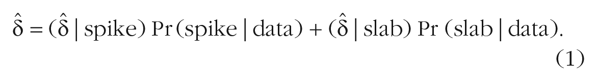
As the name suggests, the spike-and-slab model consists of two components. The first component, the spike, corresponds to the position that talking to plants does not affect their growth (i.e., $δ = 0$ ), whereas the second component, the slab, corresponds to the position that speaking to plants does affect their growth (i.e., $δ \neq 0$ ). The spike and slab are analogous to $ℋ_{0}$ and $ℋ_{1}$ discussed above. Both components are commonly deemed a priori equally likely such that the prior probability for each component is one half. One can assign prior probabilities other than one half if this is motivated by prior research, prior data, or existing theories (e.g., Wilson & Wixted, 2018). After observing the data, the prior probabilities (Pr) of both components, Pr (spike) and Pr (slab), are updated to posterior probabilities, Pr (spike | data) and Pr (slab | data).

By applying the spike-and-slab model, we learn about the relative plausibility of the two components; in addition, the spike-and-slab model produces a marginal estimate of effect size—a weighted combination of effect sizes from the spike and from the slab (for mathematical detail, see the Appendix in the Supplemental Material available online). In other words, the spike-and-slab model yields an overall effect size averaged across the spike and the slab, with averaging weights determined by the respective posterior probabilities:

\hat{δ} = (\hat{δ} | spike) \Pr (spike | data) + (\hat{δ} | slab) \Pr (slab | data) .

(1)

Marginalizing across model components according to their posterior plausibility is a uniquely Bayesian operation, and this is the statistical framework we adopt in this article (for an accessible introduction to Bayesian inference, see Vandekerckhove et al., 2018). Researchers who prefer a frequentist approach can accomplish shrinkage by using penalized maximum likelihood methods such as least absolute shrinkage and selection operator and ridge regression (Tibshirani et al., 2005). Another option open to frequentists is to marginalize across the spike and the slab, for instance by using the Akaike information criterion (AIC; Akaike, 1973) and defining the averaging weights as follows. Let $Δ AIC = (AIC | spike) - (AIC | slab)$ , the difference in AIC between the spike and the slab. Next we use the Akaike weight, $w_{spike},$ as a substitute for the posterior probability of the spike: $w_{spike} = \exp (- 1 / 2 Δ AIC) / (1 + \exp (- 1 / 2 Δ AIC))$ (Burnham & Anderson, 2002; Wagenmakers & Farrell, 2004). The substitute for the posterior probability of the slab is simply $w_{slab} = 1 - w_{spike}$ .

Note that when the spike is located at $δ = 0$ , as is usually the case, then $(\hat{δ} | spike) \Pr (spike | data) = 0$ , and consequently, Equation 1 simplifies to

\hat{δ} = (\hat{δ} | slab) \Pr (slab | data) .

(2)

This equation shows that the spike-and-slab estimate $\hat{δ}$ equals the estimate that is generally recommended in reporting guidelines, $(\hat{δ} | slab)$ , but reduced by the posterior probability for $ℋ_{1}$ . This shrinkage toward zero becomes negligible when the posterior probability for $ℋ_{1}$ approaches 1.

To illustrate both the overestimation and the spike-and-slab model, we reanalyze the fictitious data from Figure 1. R code for the analysis is available at https://osf.io/uq8st/. Remember that the frequentist point estimate for the effect size conditional on $ℋ_{1}$ , or the slab, was $\hat{δ} = 0.30$ , with 95% CI = [0.02, 0.58]. The Bayesian equivalent is $\hat{δ} = 0.29$ , with 95% credible interval (CRI) = [0.02, 0.57]. Figure 2 contrasts this Bayesian slab-only estimate against the spike-and-slab estimate.

Fig. 2.

The spike-and-slab model. The black line represents the posterior distribution of effect size given the slab (i.e., the effect is nonzero). The posterior is scaled so that its mode ( $\hat{δ} = 0.29$ ) equals the posterior probability of the alternative model (i.e., $p (slab | data) = 0.48$ ). The gray line represents the posterior probability of the spike (i.e., $\hat{δ} = 0$ : the effect is absent). The error bars and dots above the density show 95% credible intervals and the posterior mean for the slab-only model and for the spike-and-slab model.

Compared with the traditional results based only on the slab, the posterior mean and central 95% CRI of the spike-and-slab model are shrunken toward zero (i.e., 0.14, 95% CRI = [0.00, 0.48] vs. 0.29, 95% CRI = [0.02, 0.57]). This shrinkage is due to the nonnegligible probability that the effect is absent. Here, the posterior probability of the spike after seeing the data, 0.52, is almost identical to its prior probability. In Figure 2, the plausibility that the effect is absent is represented by the height of the spike, and the uncertainty about the effect’s magnitude, given that it is present, is represented by the width of the slab. Note that if the posterior probability of the spike was reduced, the spike-and-slab results would approach those of the slab-only model.

The Influence of the Spike

In the fictitious example, the spike-and-slab model reduces the estimated effect size by shrinking estimates of effect size toward zero. The result may not be surprising given that the effect was small. However, it makes one wonder to what extent the spike-and-slab model helps with estimation. What are the differences between a slab-only model and the spike-and-slab model? In this section, we illustrate how the estimated effect size shrinks toward zero under various circumstances. We visualize the shrinkage as a function of the observed effect size, the prior on the standard deviation of effect size under the slab, the sample size, and the prior probability of the spike. We chose these parameters because the posterior distribution is fully determined by these quantities (see the Appendix in the Supplemental Material).

Figure 3 shows the relation between the observed effect size and the estimated effect size for the slab and for the spike-and-slab models for 40 observations and 100 observations. All plots show that a smaller prior standard deviation of the slab induces some shrinkage toward zero. This effect is most obvious in the top left panel, and it makes sense because a small prior standard deviation implies there is more prior mass near the mean of the prior, which is zero. This influence of the prior standard deviation is typically referred to as prior shrinkage, and it intrinsic to a Bayesian approach but not to the spike-and-slab model. Comparing the plots between the two columns illustrates the influence of the spike; whenever the observed effect size is near zero, the estimate is shrunken toward zero in the right column but not in the left column. However, when the observed effect size is far from zero, there is little additional shrinkage to the prior shrinkage.

Fig. 3.

Observed effect size versus posterior mean for different model components and prior standard deviations. The left column shows inference based on the slab-only model, and the right column shows inference based on the spike-and-slab model. In the top row, the sample size was 40, and in the bottom row, the sample size was 100. Different lines represent different standard deviations for the prior distribution on $δ$ . The prior probability of the spike was one half. Inspired by Figure 5 of Rouder et al. (2018).

The shrinkage in the spike-and-slab model can be explained in the following way. Whenever the observed effect size is small, the data are well described by an effect size of zero, and thus the posterior probability of the spike is substantial. As a result, the marginal estimate is shrunken toward the spike’s estimate, zero. In contrast, when the observed effect size is large, the data are poorly described by an effect size of zero and the posterior probability of the spike is negligible. As a consequence, the estimate of the spike-and-slab is practically equivalent to the estimate of the slab. The plots in the right column of Figure 3 show the effect of sample size on the shrinkage. For the bottom right plot, $N = 100$ . If the observed effect size is small, then the estimate is still shrunken toward zero, but as the observed effect size grows, the shrinkage decreases much more quickly than in the top right plot, where $N = 40$ . This makes sense from a signal-detection perspective. If the observed effect size is, for example, 0.3 after 40 observations, the posterior probability of the spike is substantial. However, after collecting 60 additional observations, while the observed effect size remains 0.3, the posterior probability of the spike decreases as it becomes increasingly less probable that the data-generating model had an effect size of zero.

Next, we explore the relationship between shrinkage and the prior probability of the spike. Figure 4 shows the shrinkage for various prior probabilities. The smaller the prior probability of the spike, the less the effect size is shrunken toward zero. If the prior probability is small, then the spike was a priori implausible, and less evidence is needed to make its influence negligible.

Fig. 4.

Observed effect ( $x$ -axis) versus the posterior mean of the spike-and-slab model ( $y$ -axis). The different lines represent different prior probabilities of the spike. The figure is based on 40 observations with a prior standard deviation of one.

Empirical Example: Reanalysis of Two Minds

We now highlight how the spike-and-slab approach can be used in psychological practice by reanalyzing the results of Heycke et al. (2018), who conducted two registered replications of Rydell et al. (2006). We first briefly explain the design of the study before reanalyzing the explicit evaluation and implicit evaluation analyses with a spike-and-slab model. For a detailed description, see the Procedure section in Heycke et al. (2018). Finally, we provide a robustness analysis.

The goal of Heycke et al. (2018) was to replicate key evidence for implicit-attitude formation. In the original study, Rydell et al. (2006) reported that attitudes induced by subliminal primes manifest when they are assessed by an implicit-attitude measure and that attitudes induced by supraliminal cues manifest when they are assessed by an explicit-attitude measure. This finding corresponds to a perhaps surprising dissociation of implicit- and explicit-attitude measures. In the Heycke et al. experiments, participants were briefly flashed a positive or negative prime followed by an image of a person. Next, several behavioral descriptions that were either negative or positive appeared with the image of the person (e.g., “Bob cheated during a poker game”). Afterward, participants explicitly evaluated the target person and performed an implicit association task (IAT). In total, data of 51 participants were analyzed. Heycke et al. could not find the dissociation between explicit- and implicit-attitude measures. They found that although positive descriptions resulted in a more favorable explicit evaluation than negative descriptions, positive subliminal primes did not result in more favorable IAT scores than negative subliminal primes. In contrast, both explicit- and implicit-attitude measures were in line with the explicit descriptions they learned during the experiment.

Explicit evaluation

In the analysis of the explicit evaluations, Heycke et al. (2018, p. 10) conducted a paired t test and concluded that the rating of the target character is more positive if positive information is shown before negative information: $t (27) = 11.52$ , $p < . 001$ ; ${BF}_{10} = 1.37 \times 10^{9}$ , $d = 2.09$ , 95% highest density interval (HDI) = $[1.41, 2.79]$ .⁴ The magnitude of the effect is large, and thus a spike-and-slab reanalysis yields practically the same results: $\hat{δ} = 2.10$ , 95% CRI = [1.74, 2.47].⁵

Implicit evaluation

In the analysis of the IAT, Heycke et al. (2018, p. 10) conducted a paired t test and concluded that when negative primes were presented before positive primes, there was some indication that the IAT rating became more negative: $t (27) = - 2.54$ , $p = . 017$ , ${BF}_{10} = 2.92$ , $d = - 0.44$ , 95% HDI = $[- 0.83, - 0.06]$ . Here, the magnitude of the effect is smaller, and as a consequence, the results from the spike-and-slab reanalysis are more conservative: $\hat{δ} = - 0.35$ , 95% CRI = [ $- 0.75$ , 0.00]. The estimate of effect size is shrunken toward zero because the spike provides a reasonable account of the data, $\Pr (spike | data) = 0.25$ .

Robustness analysis

In the reanalyses above, the prior probability of the spike was set to 0.5. One might wonder how robust or how volatile the results are to changes in the prior probability of the spike. Figure 5 visualizes the influence of the prior on the spike. In the left panel that shows the explicit evaluation data, the different estimates for different prior probabilities are practically identical. For this analysis, the data dominate the prior. In contrast, in the right panel that shows the implicit evaluation data, the prior probability of the spike has a large impact on the results. Here, the data are less informative, and the prior has more influence. The adaptive shrinkage is a key feature of the spike-and-slab model, that is, the amount of shrinkage depends on the posterior plausibility of the spike. Note that in the right panel, the 95% CI becomes asymmetric as the prior, and therefore also the posterior probability of the spike, increases. It may appear that the CI is bounded by zero; however, this is a property of this particular data set. Had the observations been closer to zero, then the CI would have also contained negative values (e.g., the posterior mass in Fig. 2 is not zero for negative values of effect size).

Fig. 5.

Robustness analysis that shows the prior probability of the spike (x-axis) versus spike-and-slab estimates (y-axis) for the explicit evaluation (left) and the implicit evaluation (right). Solid points show the point estimate of the spike-and-slab model, and the gray area represents the accompanying 95% credible interval. The green horizontal dashed line shows the estimate of the slab.

Discussion

Standard estimates of effect size ignore the null hypothesis and are therefore overconfident, that is, farther away from zero than they should be. The spike-and-slab model tempers the enthusiasm that the standard estimates instill by explicitly considering the possibility that an effect is absent (Robinson, 2019; Rouder et al., 2018). The core idea dates back to Jeffreys (1939; see also Jeffreys, 1961, p. 365; Ly & Wagenmakers, 2020); nonetheless, it has been largely ignored in empirical practice, statistical education, and journal guidelines. We believe the spike-and-slab model is a useful statistical tool to make the interpretation of effect size estimates more robust. The spike-and-slab model optimally shrinks effect sizes with ambiguous statistical support toward zero. This data-driven statistical skepticism is appropriate regardless of whether researchers follow good research practices, for example, preregistering study design and analysis.

What if all null hypotheses are false?

The spike-and-slab approach clashes with the popular estimation mind-set, in which it is argued that statistical significance should be abandoned in favor of estimation (Cumming, 2014; Cumming & Calin-Jageman, 2016; McShane et al., 2019; Valentine et al., 2015). One argument to forgo hypothesis testing is that all null hypotheses are false (Cohen, 1990; Meehl, 1978), and therefore there is no need to consider a component that states that an effect is exactly zero. The statistical counterargument is that even if point null hypotheses are false, they are still mathematically convenient approximations to more complex hypotheses that allow mass on an interval close to zero (i.e., perinull hypotheses; Berger & Delampady, 1987; George & McCulloch, 1993; Ly et al., 2020). Thus, from a pragmatic perspective, it is irrelevant whether null hypotheses are exactly true: In the spike-and-slab model, a narrow interval around zero will shrink estimates toward zero almost as much as the point null spike component will.

When can the spike be ignored?

There are two scenarios in which the presence of the spike can safely be ignored. First, the spike may be deeply implausible. This happens most often in problems of pure estimation, such as when determining the relative popularity of two politicians or the proportion of Japanese cars on the streets of New York. In such cases, no value or interval needs to be singled out for special attention. Second, the data, or even data from prior studies, may provide overwhelming evidence that an effect is present, as in the reanalysis of the explicit evaluation data. When this happens, the results from a spike-and-slab model become virtually identical to those of a slab-only model: The inclusion of the spike offers no benefit, but neither does it come with a statistical cost.

Conclusion

Standard methods for estimating effect size produce results that are overly optimistic. This tendency toward high estimates can be corrected by applying the spike-and-slab model that explicitly takes into account the possibility that the effect is absent. The spike-and-slab approach is not meant as a tool to downplay other researchers’ findings that one disagrees with. Instead, it provides a more robust estimate of the size of an effect of high-quality studies whenever null and alternative hypothesis are plausible. We believe that the approach allows researchers a more nuanced interpretation of their own results taking into account the plausibility that there is no effect.

Supplemental Material

sj-pdf-1-amp-10.1177_2515245921992035 – Supplemental material for A Cautionary Note on Estimating Effect Size

Supplemental material, sj-pdf-1-amp-10.1177_2515245921992035 for A Cautionary Note on Estimating Effect Size by Don van den Bergh, Julia M. Haaf, Alexander Ly, Jeffrey N. Rouder and Eric-Jan Wagenmakers in Advances in Methods and Practices in Psychological Science

Footnotes

Transparency

Action Editor: Brent Donnellan

Editor: Daniel J. Simons

Author Contributions

D. van den Bergh and J. M. Haaf drafted an initial version of the manuscript. D. van den Bergh conducted the reanalysis. J. N. Rouder shared and helped with R code for the spike-and-slab model. All authors reviewed and revised the manuscript jointly and approved the final manuscript for submission.

ORCID iDs

Don van den Bergh

Julia M. Haaf

Jeffrey N. Rouder

Eric-Jan Wagenmakers

Supplemental Material

Additional supporting information can be found at

Notes

References

Akaike

(1973). Information theory as an extension of the maximum likelihood principle. In Petrov

B. N.

Csaki

(Eds.), Second international symposium on information theory (pp. 267–281). Akademiai Kiado.

Bainter

S. A.

McCauley

T. G.

Wager

Losin

E. A. R.

(2020). Improving practices for selecting a subset of important predictors in psychology: An application to predicting pain. Advances in Methods and Practices in Psychological Science, 3(1), 66–80.

Berger

J. O.

Delampady

(1987). Testing precise hypotheses. Statistical Science, 2, 317–352.

Burnham

K. P.

Anderson

D. R.

(2002). Model selection and multimodel inference: A practical information–theoretic approach (2nd ed.). Springer Verlag.

Clyde

M. A.

Desimone

Parmigiani

(1996). Prediction via orthogonalized model mixing. Journal of the American Statistical Association, 91(435), 1197–1208.

Cohen

(1990). Things I have learned (thus far). American Psychologist, 45, 1304–1312.

Cumming

(2014). The new statistics: Why and how. Psychological Science, 25, 7–29.

Cumming

Calin-Jageman

(2016). Introduction to the new statistics: Estimation, open science, and beyond. Routledge.

Davis-Stober

C. P.

Dana

Rouder

J. N.

(2018). Estimation accuracy in the psychological sciences. PLOS ONE, 13(11), Article e0207239. https://doi.org/10.1371/journal.pone.0207239

10.

Efron

Morris

(1977). Stein’s paradox in statistics. Scientific American, 236, 119–127.

11.

George

E. I.

McCulloch

R. E.

(1993). Variable selection via Gibbs sampling. Journal of the American Statistical Association, 88(423), 881–889.

12.

Geweke

(1996). Variable selection and model comparison in regression. In Bernardo

J. M.

Berger

J. O.

Dawid

A. P.

Smith

A. F. M.

(Eds.), Bayesian statistics 5 (pp. 609–620). Clarendon Press.

13.

Grant

D. A.

(1962). Testing the null hypothesis and the strategy and tactics of investigating theoretical models. Psychological Review, 69, 54–61.

14.

Harrington

D’Agostino

R. B.

Sr. Gatsonis

Hogan

J. W.

Hunter

D. J.

Normand

S.-L. T.

Drazen

J. M.

Hamel

M. B.

(2019). New guidelines for statistical reporting in the Journal. The New England Journal of Medicine, 381(3), 285–286. https://doi.org/10.1056/NEJMe1906559

15.

Heycke

Gehrmann

Haaf

J. M.

Stahl

(2018). Of two minds or one? A registered replication of Rydell et al. (2006). Cognition and Emotion, 32(8), 1708–1727.

16.

Ishwaran

Rao

J. S.

(2005). Spike and slab variable selection: Frequentist and Bayesian strategies. The Annals of Statistics, 33(2), 730–773. https://doi.org/10.1214/009053604000001147

17.

Iverson

G. J.

Wagenmakers

E.-J.

Lee

M. D.

(2010). A model averaging approach to replication: The case of prep. Psychological Methods, 15, 172–181.

18.

Jeffreys

(1939). Theory of probability (1st ed.). Oxford University Press.

19.

Jeffreys

(1961). Theory of probability (3rd ed.). Oxford University Press.

20.

Loftus

G. R.

(1996). Psychology will be a much better science when we change the way we analyze data. Current Directions in Psychological Science, 5, 161–171.

21.

Stefan

van Doorn

Dablander

van den Bergh

Sarafoglou

Kucharskỳ

Š.

Derks

Gronau

Q. F.

Komarlu Narendra Gupta

A. R.

Boehm

van Kesteren

E.-J.

Hinne

Matzke

Mars-man

Wagenmakers

E.-J.

(2020). The Bayesian methodology of Sir Harold Jeffreys as a practical alternative to the p-value hypothesis test. Computational Brain & Behavior, 3, 153–161.

22.

Wagenmakers

E.-J.

(2020). Bayes factors for peri-null hypotheses. arXiv. Retrieved from https://arxiv.org/pdf/2102.07162.pdf

23.

McShane

B. B.

Gal

Gelman

Robert

Tackett

J. L.

(2019). Abandon statistical significance. The American Statistician, 73(Supp. 1), 235–245.

24.

Meehl

P. E.

(1978). Theoretical risks and tabular asterisks: Sir Karl, Sir Ronald, and the slow progress of soft psychology. Journal of Consulting and Clinical Psychology, 46, 806–834.

25.

Mitchell

T. J.

Beauchamp

J. J.

(1988). Bayesian variable selection in linear regression. Journal of the American Statistical Association, 83(404), 1023–1032.

26.

Morey

R. D.

Hoekstra

Rouder

J. N.

Lee

M. D.

Wagenmakers

E.-J.

(2016). The fallacy of placing confidence in confidence intervals. Psychonomic Bulletin & Review, 23, 103–123.

27.

O’Hara

R. B.

Sillanpää

M. J.

, et al. (2009). A review of Bayesian variable selection methods: What, how and which. Bayesian Analysis, 4(1), 85–117. https://doi.org/10.1214/09-BA403

28.

Robinson

G. K.

(2019). What properties might statistical inferences reasonably be expected to have?—Crisis and resolution in statistical inference. The American Statistician, 73, 243–252.

29.

Rouder

J. N.

Haaf

J. M.

Vandekerckhove

(2018). Bayesian inference for psychology, part IV: Parameter estimation and Bayes factors. Psychonomic Bulletin & Review, 25, 102–113.

30.

Rouder

J. N.

(2005). An introduction to Bayesian hierarchical models with an application in the theory of signal detection. Psychonomic Bulletin & Review, 12, 573–604.

31.

Rydell

R. J.

McConnell

A. R.

Mackie

D. M.

Strain

L. M.

(2006). Of two minds: Forming and changing valence-inconsistent implicit and explicit attitudes. Psychological Science, 17(11), 954–958.

32.

Shiffrin

R. M.

Lee

M. D.

Kim

Wagenmakers

E.-J.

(2008). A survey of model evaluation approaches with a tutorial on hierarchical Bayesian methods. Cognitive Science, 32, 1248–1284.

33.

Tibshirani

Saunders

Rosset

Zhu

Knight

(2005). Sparsity and smoothness via the fused lasso. Journal of the Royal Statistical Society: Series B (Statistical Methodology), 67(1), 91–108.

34.

Valentine

J. C.

Aloe

A. M.

Lau

T. S.

(2015). Life after NHST: How to describe your data without “p-ing” everywhere. Basic and Applied Social Psychology, 37(5), 260–273.

35.

Vandekerckhove

Rouder

J. N.

Kruschke

J. K.

(Eds.). (2018). Editorial: Bayesian methods for advancing psychological science. Psychonomic Bulletin & Review, 25, 1–4.

36.

van Erp

Oberski

D. L.

Mulder

(2019). Shrinkage priors for Bayesian penalized regression. Journal of Mathematical Psychology, 89, 31–50.

37.

Wagenmakers

E.-J.

Farrell

(2004). AIC model selection using Akaike weights. Psychonomic Bulletin & Review, 11, 192–196.

38.

Wilson

B. M.

Wixted

J. T.

(2018). The prior odds of testing a true effect in cognitive and social psychology. Advances in Methods and Practices in Psychological Science, 1(2), 186–197.

39.

C.-H.

Prado

Ombao

Rowe

(2018). A Bayesian variable selection approach yields improved detection of brain activation from complex-valued fMRI. Journal of the American Statistical Association, 113(524), 1395–1410.

Supplementary Material

Please find the following supplemental material available below.

For Open Access articles published under a Creative Commons License, all supplemental material carries the same license as the article it is associated with.

For non-Open Access articles published, all supplemental material carries a non-exclusive license, and permission requests for re-use of supplemental material or any part of supplemental material shall be sent directly to the copyright owner as specified in the copyright notice associated with the article.

0.00 MB

0.06 MB