Sage Journals: Discover world-class research

Abstract

Replication is an important contemporary issue in psychological research, and there is great interest in ways of assessing replicability, in particular, retrospectively via prior studies. The average power of a set of prior studies is a quantity that has attracted considerable attention for this purpose, and techniques to estimate this quantity via a meta-analytic approach have recently been proposed. In this article, we have two aims. First, we clarify the nature of average power and its implications for replicability. We explain that average power is not relevant to the replicability of actual prospective replication studies. Instead, it relates to efforts in the history of science to catalogue the power of prior studies. Second, we evaluate the statistical properties of point estimates and interval estimates of average power obtained via the meta-analytic approach. We find that point estimates of average power are too variable and inaccurate for use in application. We also find that the width of interval estimates of average power depends on the corresponding point estimates; consequently, the width of an interval estimate of average power cannot serve as an independent measure of the precision of the point estimate. Our findings resolve a seeming puzzle posed by three estimates of the average power of the power-posing literature obtained via the meta-analytic approach.

Keywords

power effect size meta-analysis publication bias history of science open materials

Replication is an important contemporary issue in psychological research, and several recent efforts have been devoted to assessing the replicability of one phenomenon or a small number of phenomena (Klein et al., 2014; Klein et al., 2018; Simons, Holcombe, & Spellman, 2014), as well as the domain as a whole (Open Science Collaboration, 2015). Unfortunately, these prospective replication efforts involve heroic levels of coordination, require tremendous resources, and are relatively slow. Consequently, there is great interest in alternative ways of assessing replicability, in particular, retrospectively via prior studies.

The average power of a set of prior studies is a quantity that has attracted considerable attention for this purpose. Indeed, average power has been labeled a “replicability estimate” (Brunner & Schimmack, 2016; Schimmack & Brunner, 2017) and described as estimating the rate of replicability “if the same studies were run again” (Simmons & Simonsohn, 2017, p. 690). Further, techniques to estimate this quantity via a meta-analytic approach have recently been proposed (Brunner & Schimmack, 2016; Simonsohn, Nelson, & Simmons, 2014).

In this article, we have two aims. First, we clarify the nature of average power and its implications for replicability. We explain that average power is not relevant to the replicability of actual prospective replication studies. Instead, it relates to efforts in the history of science to catalogue the power of prior studies (Cohen, 1962; Rossi, 1990; Sedlmeier & Gigerenzer, 1989).

Second, we evaluate the statistical properties of point estimates and interval estimates of average power obtained via the meta-analytic approach. We find that point estimates of average power are too variable and inaccurate for use in application. We also find that the width of interval estimates of average power depends on the corresponding point estimates; consequently, the width of an interval estimate of average power cannot serve as an independent measure of the precision of the point estimate.

As we discuss, our findings resolve a seeming puzzle posed by three estimates of the average power of the power-posing literature obtained via the meta-analytic approach. Specifically, the 95% interval estimates of average power reported by Cuddy, Schultz, and Fosse (2018) and Schimmack and Brunner (2017) are more than 3 times the width of the 95% interval estimate reported by Simmons and Simonsohn (2017)—despite the fact that the meta-analyses conducted by Cuddy et al. and Schimmack and Brunner included all 33 studies included in the meta-analysis of Simmons and Simonsohn, as well as 20 additional ones. When considered alongside the results reported by Cuddy et al. and Schimmack and Brunner, our findings strongly suggest that the interval estimate reported by Simmons and Simonsohn and obtained via the so-called p-curve meta-analytic model is optimistically narrow if taken as a measure of precision.

Disclosures

Code for our analyses is available both as Supplemental Material (http://journals.sagepub.com/doi/suppl/10.1177/2515245920902370) and at the Open Science Framework (https://osf.io/3gyu7/).

Average Power and Replicability

The power of a study is, by definition, the probability that the study yields results that are statistically significant in the classical frequentist repeated sampling framework. Put differently but equivalently, the power of a study is the long-run frequency that the study yields results that are statistically significant if the study could be repeated infinitely many times such that the only difference among the repetitions is the sampling error realized.

Similarly, the average power of a set of prior studies is, by definition, the average (i.e., arithmetic mean) of the power of each study in the set. Consequently, average power gives the fraction of the prior studies that in expectation yield—or, equivalently, the probability that one prior study chosen randomly and uniformly from the set yields—results that are statistically significant in the classical frequentist repeated sampling framework.

Perhaps because of this, it has been claimed that average power is relevant to the replicability of actual prospective replication studies (Brunner & Schimmack, 2016; Schimmack & Brunner, 2017; Simmons & Simonsohn, 2017). However, for at least three reasons, it is not. First, even were direct or exact replication possible in psychological research such that the classical frequentist repeated sampling framework might apply, average power is wed to prior study design choices, including sample sizes, whereas actual prospective replication studies are not (see, e.g., Open Science Collaboration, 2015, which employed larger sample sizes than prior studies so as to increase power).

Second, it has long been argued that direct or exact replication is not possible in psychological research (Brandt et al., 2014; Fabrigar & Wegener, 2016; Rosenthal, 1991; Stroebe & Strack, 2014); instead, effect sizes vary from one study of a given phenomenon to the next such that the classical frequentist repeated sampling framework does not apply. Recent empirical evidence strongly supports this view, documenting that heterogeneity is rife across both general (i.e., systematic or conceptual) replications (Stanley, Carter, & Doucouliagos, 2018; van Erp, Verhagen, Grasman, & Wagenmakers, 2017) and close replications (i.e., studies that use identical or very similar materials; McShane, Tackett, Böckenholt, & Gelman, 2019).

Third, the success or failure of replication need not be defined in terms of statistical significance. Indeed, the null hypothesis significance testing paradigm upon which the notion of statistical significance is based has been the subject of no small amount of criticism (see, e.g., Amrhein, Greenland, & McShane, 2019; Boring, 1919; McShane, Gal, Gelman, Robert, & Tackett, 2019; Rozenboom, 1960), and alternative definitions involving, for example, the convergence or divergence of results across multiple studies of a given phenomenon can be employed (see, e.g., Open Science Collaboration, 2015, which employed five distinct definitions).

In sum, average power is relevant to replicability if and only if replication is defined in terms of statistical significance within the classical frequentist repeated sampling framework. As this framework is both purely hypothetical and ontologically impossible, average power is not relevant to the replicability of actual prospective replication studies. It is thus misleading, if not incorrect, to label average power a “replicability estimate” (Brunner & Schimmack, 2016; Schimmack & Brunner, 2017) and to describe it as estimating the rate of replicability “if the same studies were run again” (Simmons & Simonsohn, 2017, p. 690) without this explicit qualification. Instead, average power relates to efforts in the history of science to catalogue the power of prior studies.

Estimating Average Power

The meta-analytic approach

Because the power of any study is never known, the average power of a set of prior studies is also never known. Instead, it must be estimated. A natural approach to estimating average power is to estimate the power of each study in the set and then to average these estimates. This requires an estimate of the effect size and an estimate of the sampling variance of each prior study.

Meta-analysis also requires an estimate of the effect size and the sampling variance of each prior study. It combines these across the studies to produce, among other things, a revised estimate of the effect size of each prior study that reflects the entire set of studies.

In the meta-analytic approach to estimating average power, the revised estimate of the effect size of each prior study is used in conjunction with the estimate of the sampling variance of the study to estimate the power of the study; then, these estimates of the power of each prior study are averaged to estimate average power. Insofar as the revised estimates of the effect size of each prior study constitute an improvement over the original ones, so too should the resulting estimates of the power of each study and of average power. Further, insofar as heterogeneous effect sizes, study-level moderators, publication bias, and other factors are deemed relevant, various meta-analytic techniques that attempt to account for these factors can be employed; the use of such techniques will be reflected in the revised estimate of the effect size of each prior study and thus also in the resulting estimates of the power of each study and of average power, yielding further improvement.

Given this, the meta-analytic approach to estimating average power can be seen as a multistudy analogue of the much-derided post hoc approach to estimating single-study power (Hoenig & Heisey, 2001; Yuan & Maxwell, 2005), which uses the effect size and the sampling variance observed in a study to estimate the power of the study. However, (a) by using the revised estimate of the effect size of each prior study (which reflects the entire set of studies and potentially also heterogeneous effect sizes, study-level moderators, publication bias, and other factors), rather than the effect size observed in the prior study, to estimate the power of the prior study and (b) by considering the average power of a set of studies, rather than the power of a single study, the meta-analytic approach at least has the potential to overcome some of the limitations of the post hoc approach—even though both are retrospective in nature.

In the remainder of this section, we evaluate the statistical properties of point estimates and interval estimates of average power obtained via the meta-analytic approach. Before proceeding, we note that because the direction of the effect of interest is often specified in psychological research, we focus on statistical significance (and thus power) as determined by a one-tailed test unless otherwise noted. We set size α of the test such that study results are deemed statistically significant if they have a one-tailed p value less than .025 (or, equivalently, if they are directionally consistent with the true effect and have a two-tailed p value less than .05). We note that one-tailed power and two-tailed power are virtually equal for the corresponding αs except in extreme cases when one-tailed and two-tailed power are very low or α is very high. We also note that two-tailed power is simply the sum of the one-tailed powers in the two directions. Thus, our results apply broadly to two-tailed power as well.

Point estimates of average power

Scenario 1

The most important consideration in point estimation is accuracy. Consequently, we begin by evaluating the accuracy of point estimates of average power obtained via the meta-analytic approach in the statistically most ideal scenario possible. We do so not because we view this scenario as realistic, but rather to establish a bound on the level of accuracy that one can expect to obtain. Specifically, because ideal scenarios yield optimistic assessments of accuracy, point estimates will be less accurate in more realistic scenarios. Consequently, if accurate point estimates cannot be obtained in this scenario, they cannot be obtained in more realistic scenarios and thus in application.

Given a statistical model for the observed data and an estimator of some quantity based on the observed data, the accuracy of point estimates of the quantity can be assessed via the sampling distribution of the estimates obtained from the estimator (i.e., the distribution of the estimates across repeated samples of the observed data). Specifically, if this distribution is both narrow and centered near the true value of the quantity regardless of the true value (i.e., if the estimator is both low in variance and low in bias, respectively), one will tend to obtain accurate point estimates; alternatively, if this distribution is wide or centered far away from the true value of the quantity (i.e., if the estimator is high in variance or high in bias, respectively), one will tend to obtain inaccurate point estimates.

Given this, suppose that one is interested in estimating the average power of a set of independent studies that all follow a two-condition between-subjects design, that the effect of interest is the difference between the means of the two conditions, that this difference is common across studies, that the individual-level observations are normally distributed with these respective means and known variance (which we assume without loss of generality is equal to 1 such that the effect size is on the standardized Cohen’s d scale), and that the sample size per condition is equal within each study and across studies. Further, suppose that one estimates the meta-analytic model using the maximum likelihood estimator for the correctly specified statistical model for the observed data; that is, individual study effect-size estimates (and test statistics) are modeled as independently distributed according to a normal distribution with common effect size and known variance—the classic one-parameter so-called fixed-effects meta-analytic model.

This scenario is statistically the most ideal one possible for meta-analysis—and thus for the meta-analytic approach to estimating average power—for several reasons. First, the meta-analytic model is correctly specified. Second, the meta-analytic model is as simple as possible, consisting of an extremely straightforward and well-behaved distribution (i.e., independent normal with common effect size and known variance) and requiring only a single model parameter to be estimated. Third, the meta-analytic model is estimated via the maximum likelihood estimation strategy, which possesses several optimality properties. Fourth, the sampling variance of each study is known. In fact, this scenario is so ideal that the sampling distribution of the point estimate of average power can be derived analytically (see the appendix for details).

We present the sampling distribution of the point estimate of average power, both analytically, based on Equation 4 in the appendix, and numerically, based on 10,000 samples, when the number of studies included in the meta-analysis is set to 30, the effect size is set to 0.5, and the sample size per condition in each study is set to achieve a target level of power of .5 (which requires a sample size of 31 subjects per condition in each study and which yields a realized level of power of .503 in each study and thus an average power of .503) in the left panel of Figure 1. The figure shows that the sampling distribution of the point estimate is centered around the true value of .503 but has nontrivial width; that is, the estimates are highly variable and thus not particularly accurate. For example, the 2.5% and 97.5% quantiles of the sampling distribution are .363 and .643, respectively. In other words, one is reasonably likely to obtain a point estimate of average power as low as .363 or as high as .643 when the true value is .503 even when one includes 30 studies—with a total sample size of 1,860 (30 studies × 31 subjects per condition × 2 conditions) subjects—in the meta-analysis. (Note: The median number of studies included in meta-analyses in psychological research is 12, and only 26% include more than 30 studies; van Erp et al., 2017.)

Fig. 1.

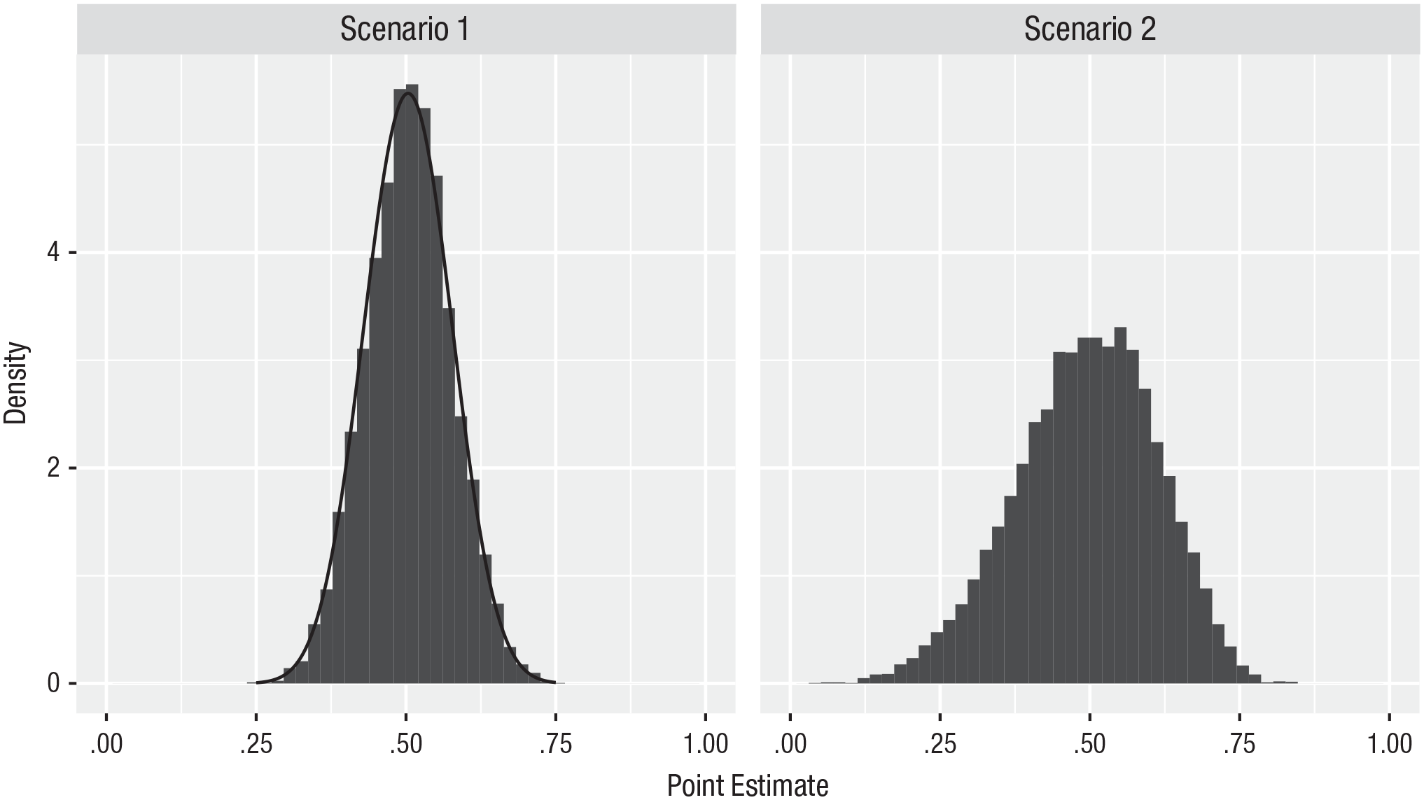
Sampling distribution of the point estimate of average power. The sampling distribution is evaluated analytically (density curve) and numerically, based on 10,000 samples (histogram). The sampling distributions are centered around the true value of .503 but have nontrivial width; that is, point estimates of average power are highly variable and thus not particularly accurate.

To assess whether these results are idiosyncratic to the number of studies, effect size, or target level of power employed, we varied the number of studies from 10 to 100 in increments of 10 and both the effect size and target level of power from 0.1 to 0.9 in increments of 0.1. The sample size per condition in each study required by each combination of effect size and target level of power and the realized level of power yielded by that sample size are provided for reference in Tables 1 and 2, respectively.

Table 1.

Sample Size per Condition

Effect size	Target level of power
Effect size	.1	.2	.3	.4	.5	.6	.7	.8	.9
0.1	93	251	413	583	769	980	1,235	1,570	2,102
0.2	24	63	104	146	193	245	309	393	526
0.3	11	28	46	65	86	109	138	175	234
0.4	6	16	26	37	49	62	78	99	132
0.5	4	11	17	24	31	40	50	63	85
0.6	3	7	12	17	22	28	35	44	59
0.7	2	6	9	12	16	20	26	33	43
0.8	2	4	7	10	13	16	20	25	33
0.9	2	4	6	8	10	13	16	20	26

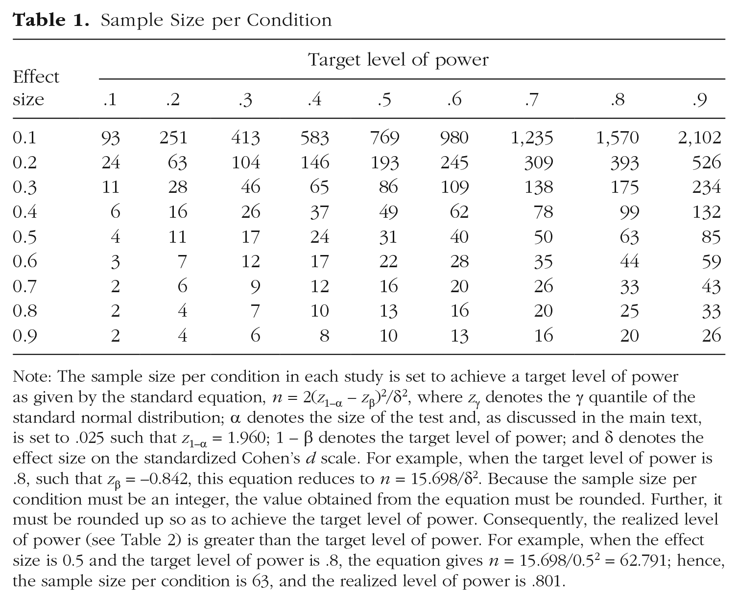
Note: The sample size per condition in each study is set to achieve a target level of power as given by the standard equation, n = 2(Z_1–α – Z_β)²/δ², where Z_γ denotes the γ quantile of the standard normal distribution; α denotes the size of the test and, as discussed in the main text, is set to .025 such that Z_1–α = 1.960; 1 – β denotes the target level of power; and δ denotes the effect size on the standardized Cohen’s d scale. For example, when the target level of power is .8, such that Z_β = −0.842, this equation reduces to n = 15.698/δ². Because the sample size per condition must be an integer, the value obtained from the equation must be rounded. Further, it must be rounded up so as to achieve the target level of power. Consequently, the realized level of power (see Table 2) is greater than the target level of power. For example, when the effect size is 0.5 and the target level of power is .8, the equation gives n = 15.698/0.5² = 62.791; hence, the sample size per condition is 63, and the realized level of power is .801.

Table 2.

Realized Level of Power

Effect size	Target level of power
Effect size	.1	.2	.3	.4	.5	.6	.7	.8	.9
0.1	.101	.201	.301	.400	.500	.600	.700	.800	.900
0.2	.103	.201	.302	.401	.502	.600	.701	.801	.900
0.3	.104	.201	.301	.401	.503	.601	.703	.801	.901
0.4	.103	.204	.302	.405	.508	.605	.705	.804	.901
0.5	.105	.216	.308	.410	.503	.609	.705	.801	.903
0.6	.110	.201	.312	.417	.512	.612	.709	.804	.903
0.7	.104	.227	.317	.403	.508	.600	.714	.812	.901
0.8	.123	.204	.322	.432	.532	.619	.716	.807	.901
0.9	.145	.246	.344	.436	.521	.631	.721	.812	.901

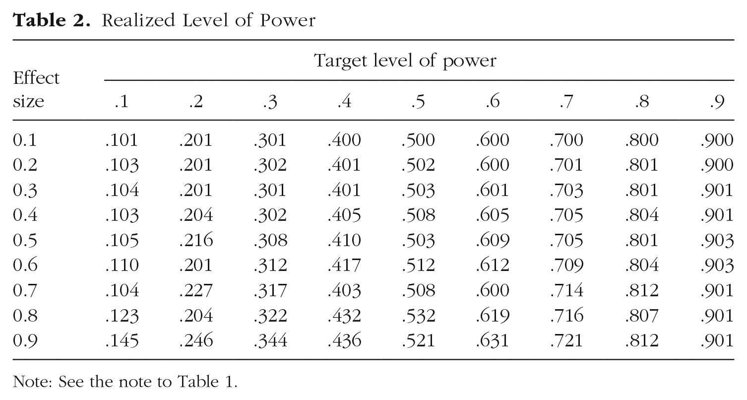
Note: See the note to Table 1.

Because it would be prohibitive to present the resulting 810 (10 numbers of studies × 9 effect sizes × 9 target levels of power) sampling distributions via histograms, we summarize each distribution by a single number that describes its variability, in particular, the difference between the 97.5% and 2.5% quantiles, which we term the 95% sampling distribution width.¹ For example, the 95% sampling distribution width of the distribution presented in the left panel of Figure 1 is .280 (.643 – .363).

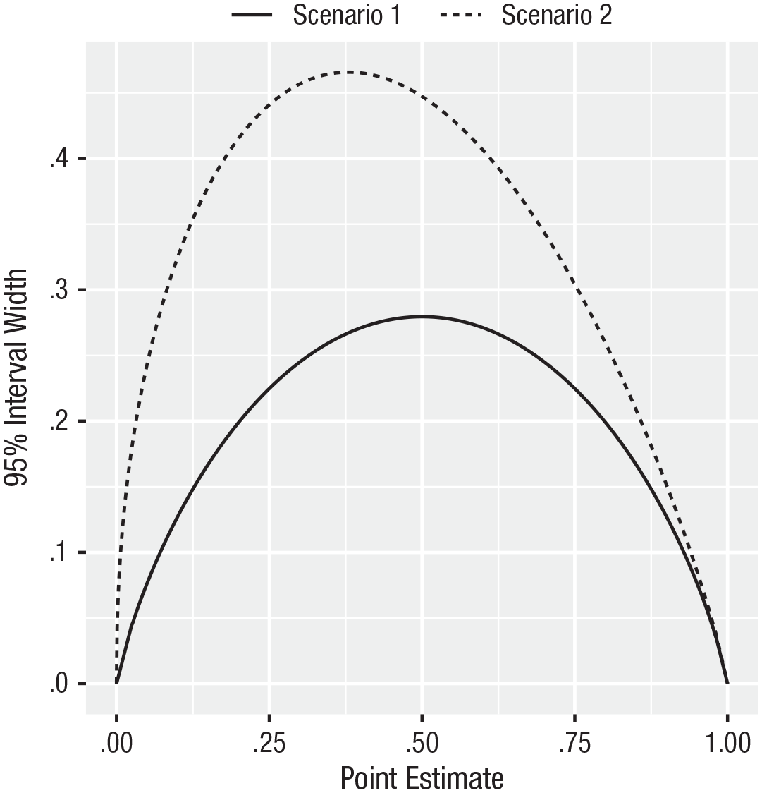
We present 95% sampling distribution widths via solid lines in Figure 2; for simplicity, we present them for only three effect sizes and three target levels of power. As shown, the effect size has no impact on the sampling distribution width; this is a direct consequence of the fact that the sample size per condition was set to achieve the target level of power. Further, the sampling distribution width is smallest when average power is low or high and largest when it is moderate; this occurs because power is bounded between 0 and 1, and, thus, when it is low or high, the sampling distribution runs up against the bound.

Fig. 2.

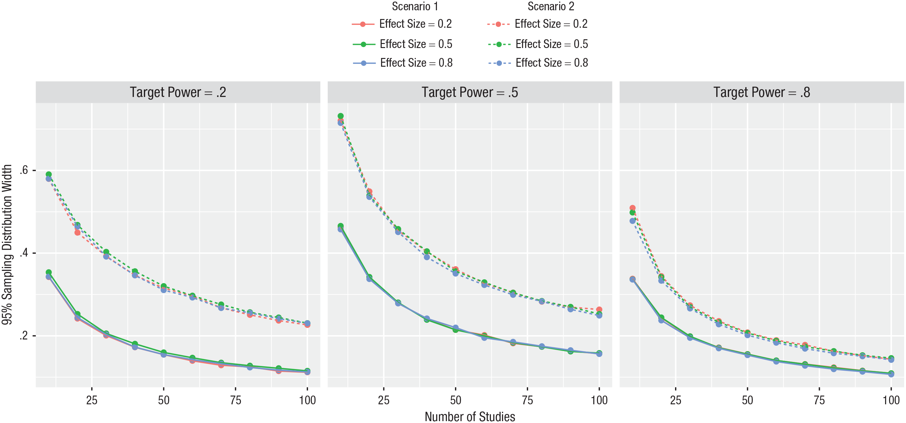
Ninety-five percent sampling distribution width. The sampling distribution width is smallest when average power is low or high and largest when it is moderate. Further, the sampling distribution width in Scenario 2 is substantially larger than the corresponding one in Scenario 1. Finally, point estimates of average power are highly variable and thus not particularly accurate.

The figure can be used to assess the degree of variability one must be prepared to face when one has a given number of studies available for estimating average power. For example, if 30 studies are available, the 95% sampling distribution width is about .2 when average power is .2, just under .3 when average power is .5, and about .2 when average power is .8. Because the true value of average power is never known, the degree of variability one must be prepared to face is the maximum 95% sampling distribution width over all values. We present these maximum values in the first row of Table 3. The table shows, for example, that one must be prepared to face a 95% sampling distribution width of .283 when 30 studies are available for estimating average power.

Table 3.

Maximum 95% Sampling Distribution Width

Scenario	Number of studies
Scenario	10	20	30	40	50	60	70	80	90	100
Scenario 1	.470	.343	.283	.245	.220	.202	.187	.176	.166	.158
Scenario 2	.732	.562	.473	.416	.373	.343	.321	.301	.286	.268

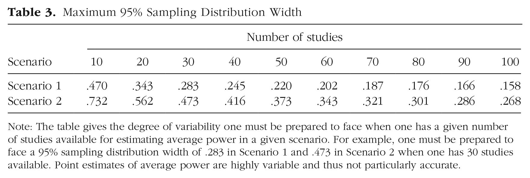
Note: The table gives the degree of variability one must be prepared to face when one has a given number of studies available for estimating average power in a given scenario. For example, one must be prepared to face a 95% sampling distribution width of .283 in Scenario 1 and .473 in Scenario 2 when one has 30 studies available. Point estimates of average power are highly variable and thus not particularly accurate.

Although what constitutes a tolerable degree of variability varies by context, we view a 95% sampling distribution width of .2 as the worst tolerable for estimating average power. As shown in the first row of Table 3, more than 60 studies are required to avoid exceeding this worst tolerable degree of variability in this scenario. Given that only 13% of meta-analyses in psychological research include more than 60 studies (van Erp et al., 2017) and that point estimates of average power will be more variable and thus less accurate in more realistic scenarios, we can conclude that point estimates of average power are too variable and inaccurate for use in application.

Before proceeding, we note that various criticisms of the post hoc approach to estimating single-study power notwithstanding, these results provide yet another—and a probative—one. Specifically, the estimator of the effect size used by the post hoc approach to estimate the power of a study is identical to the one used here when only a single study is available, and, further, this estimator is correctly specified. Consequently, the first row of Table 3 can be used to infer that point estimates of power obtained by the post hoc approach are extremely variable and thus extremely inaccurate; indeed, although not shown in the table, the maximum 95% sampling distribution width when only a single study is available is .950 in this scenario (because when the true value of power is .5 and only a single study is available, the sampling distribution of the point estimate of power is the uniform distribution on the unit interval).

Scenario 2

Given the results presented above, one might argue that there is no need to consider additional scenarios because if accurate point estimates cannot be obtained in that ideal scenario, they cannot be obtained in more realistic scenarios. Although this argument is clearly valid, recent techniques to estimate average power via the meta-analytic approach (Brunner & Schimmack, 2016; Simonsohn et al., 2014) motivated us to consider one additional scenario.

Specifically, these techniques attempt to estimate average power in a manner that attempts to address publication bias—the fact that studies with results that are statistically significant are overrepresented in the published literature relative to those with results that are not. They attempt to do so by estimating the meta-analytic model based only on studies with results that are statistically significant in a manner that accounts for this selection.² Consequently, we believe it worthwhile to evaluate point estimates of average power based only on studies with results that are statistically significant so as to determine just how much variability increases and thus accuracy decreases relative to the prior scenario.

Thus, we now evaluate point estimates of average power in a scenario that is statistically the most ideal one possible when such estimates are based only on studies with results that are statistically significant. Specifically, this scenario is identical to the prior scenario except in one regard, namely, that the meta-analytic model is estimated based only on studies with results that are statistically significant in a manner that accounts for this selection.

This scenario is statistically the most ideal one possible for meta-analysis—and thus for the meta-analytic approach to estimating average power—based only on studies with results that are statistically significant for several reasons. First, the meta-analytic model is correctly specified; that is, individual study effect-size estimates (and test statistics) are modeled as independently distributed according to a truncated normal distribution with common effect size and known variance—a one-tailed normal variant of the classic one-parameter Hedges (1984) selection model that accounts for the selection to only studies with results that are statistically significant. Second, the meta-analytic model is as simple as possible given the selection to only studies with results that are statistically significant and requires only a single model parameter to be estimated. Third, the meta-analytic model is estimated via the maximum likelihood estimation strategy, which possesses several optimality properties. Fourth, the sampling variance of each study is known.

We present the sampling distribution of the point estimate of average power numerically based on 10,000 samples when the number of studies (all with results that are statistically significant) included in the meta-analysis is set to 30, the effect size is set to 0.5, and power is set to .503 in the right panel of Figure 1. The figure shows that the sampling distribution of the point estimate is again centered around the true value of .503 but has nontrivial width; that is, the estimates are highly variable and thus not particularly accurate. For example, the 2.5% and 97.5% quantiles of the sampling distribution are .244 and .703, respectively. In other words, one is reasonably likely to obtain a point estimate of average power as low as .244 or as high as .703 when the true value is .503 even when one includes 30 studies with results that are statistically significant in the meta-analysis.

The figure shows that the distribution corresponding to this scenario is—as expected—substantially wider than the distribution corresponding to the prior scenario, even though estimates in the two scenarios are based on the same number of studies (i.e., 30 studies with results that are statistically significant in this scenario vs. 30 studies regardless of results in the prior scenario). For example, the 2.5% and 97.5% quantiles of the sampling distribution widen from .363 and .643, respectively, in the prior scenario to .244 and .703, respectively, in this scenario; put differently, the 95% sampling distribution width increases from .280 to .458. In sum, point estimates of average power are much more variable and thus much less accurate when based only on studies with results that are statistically significant.

We now consider all 810 cases considered in the prior scenario. We present 95% sampling distribution widths via dashed lines in Figure 2; for simplicity, we again present them for only three effect sizes and three target levels of power in the figure. As shown, the effect size again has no impact on the sampling distribution width; this is a direct consequence of the fact that the sample size per condition was set to achieve the target level of power. Further, the sampling distribution width is again smallest when average power is low or high and largest when it is moderate; this occurs because power is bounded between 0 and 1, and, thus, when it is low or high, the sampling distribution runs up against the bound. Finally, the sampling distribution width in this scenario is substantially larger than the corresponding one in the prior scenario even though the estimates in the two scenarios are based on the same number of studies; that is, point estimates of average power are much more variable and thus much less accurate when based only on studies with results that are statistically significant. However, the difference between the two scenarios decreases as average power increases; this occurs because as average power increases, publication bias decreases and thus this scenario converges to the prior scenario.

The figure can be used to assess the degree of variability one must be prepared to face when one has a given number of studies with results that are statistically significant available for estimating average power (i.e., the maximum 95% sampling distribution width). We present these maximum values in the second row of Table 3. The table shows, for example, that one must be prepared to face a 95% sampling distribution width of .473 when 30 studies with results that are statistically significant are available for estimating average power. Further, it is, for all intents and purposes, not possible to avoid exceeding the worst tolerable degree of variability (i.e., .2) when estimating average power based only on studies with results that are statistically significant. Given that point estimates of average power based only on studies with results that are statistically significant will be more variable and thus less accurate in more realistic scenarios, we conclude that such estimates—featured by recent techniques (Brunner & Schimmack, 2016; Simonsohn et al., 2014)—are extremely variable and inaccurate. We therefore reiterate our conclusion that point estimates of average power are too variable and inaccurate for use in application.

Interval estimates of average power

In this subsection, we evaluate interval estimates of average power in the context of Scenarios 1 and 2. Under one-parameter meta-analytic models like those considered in the two scenarios, estimating a confidence interval for average power is trivial because there is a one-to-one monotonic relationship between the parameter of the meta-analytic model and average power. Consequently, one can simply (a) estimate the usual confidence interval for the parameter of the meta-analytic model and (b) use the bounds of that confidence interval to estimate a confidence interval for average power.³

In the context of Scenarios 1 and 2, interval estimates of average power have two desirable properties. First, they are valid; that is, nominal (1 – α) × 100% interval estimates cover the true value of average power (1 – α) × 100% of the time. Second, the expected width of nominal (1 – α) × 100% interval estimates matches the corresponding (1 – α) × 100% sampling distribution width; among other things, this means that if we had plotted the expected width of the 95% interval estimates in Figure 2 rather than the 95% sampling distribution width, the figure would look identical.

However, interval estimates of average power have one very undesirable property: The width of such interval estimates depends on the corresponding point estimates. To illustrate this, we have plotted the width of the 95% interval estimate of average power against the corresponding point estimate when the number of studies included in the meta-analysis is set to 30 in Figure 3; we note that the relationship between these two quantities depends on neither the effect size nor the target level of power. The figure shows a strong inverse U-shaped relationship between the two quantities. Specifically, low and high point estimates of average power are accompanied by narrow interval estimates of average power, whereas moderate point estimates are accompanied by wide interval estimates—regardless of the true value of average power.

Fig. 3.

Width of the 95% interval estimate of average power versus the corresponding point estimate. The width of interval estimates of average power depends on the corresponding point estimates. Consequently, the width of an interval estimate of average power cannot serve as an independent measure of the precision of the point estimate.

In Scenario 1, this inverse U-shaped relationship holds because of the S-shaped relationship between effect size and power. Specifically, although the width of the interval estimate of the meta-analytic effect-size parameter does not depend on the corresponding point estimate of the meta-analytic effect-size parameter in this scenario, this S-shaped relationship causes the width of the interval estimate of average power to depend on the corresponding point estimate of average power. In Scenario 2, this inverse U-shaped relationship is exacerbated because in this scenario, the width of the interval estimate of the meta-analytic effect-size parameter also depends on the corresponding point estimate of the meta-analytic effect-size parameter.

This inverse U-shaped relationship is particularly problematic because point estimates of average power are highly variable. Specifically, although point estimates of average power can in theory span the entire unit interval, they would in practice span a very narrow subset of it were they highly stable; consequently, the inverse U-shaped relationship would not be made manifest all that much. However, point estimates of average power are instead highly variable and thus in practice span a relatively wide subset of the unit interval; consequently, the inverse U-shaped relationship is made manifest.

The implication of this is that the width of an interval estimate of average power cannot serve as an independent measure of the precision of the point estimate. In particular, a narrow interval estimate of average power accompanied by a relatively low or high point estimate of average power does not necessarily indicate a precise point estimate; instead, it reflects the low or high point estimate irrespective of the true value of average power.

For example, suppose that one estimates a meta-analytic model based on 30 studies with results that are statistically significant, as in Scenario 2, and obtains a point estimate of average power of .1. In this case, the width of the interval estimate of average power will be about .3 (see Fig. 3). However, because point estimates of average power are highly variable, the true value of average power might actually be, say, .3, and had average power been estimated at this true value, one would have obtained an interval estimate of average power with width of about .45 (see Fig. 3). In other words, the relative narrowness of the interval estimate reflects not precision but simply the low point estimate of .1.

Additional scenarios

In the appendix, we further investigate estimates of average power obtained via the meta-analytic approach by means of an analytic treatment that generalizes the two scenarios along three lines, namely, to allow

(a) The sampling variance of each study to be treated as unknown (such that individual study test statistics are independently distributed according to a noncentral t distribution with common effect size) rather than as known (such that individual study test statistics are independently distributed according to a normal distribution with common effect size and known variance), as in Scenarios 1 and 2.

(b) The likelihood that studies with results that are not statistically significant relative to those with results that are statistically significant are included in the meta-analysis to vary, rather than to be fixed at 1, as in Scenario 1, or 0, as in Scenario 2.

(c) This relative likelihood to be treated as unknown (in which case it is estimated), rather than as known, as in Scenarios 1 and 2.

In any case, the meta-analytic model is estimated using the maximum likelihood estimator for the correctly specified statistical model for the observed data—a one-tailed normal (or noncentral t, as appropriate) variant of the classic Iyengar and Greenhouse (1988) selection model.

Readers interested in exploring Scenarios 1 and 2, as well as these more general scenarios, can do so at a website available at https://blakemcshane.shinyapps.io/averagepower.

Application to Power Posing

As noted in our introduction, three estimates of the average power of the power-posing literature have been obtained via the meta-analytic approach⁴:

(a) Simmons and Simonsohn (2017) estimated average power at .05, 95% confidence interval = [.05, .18], based on a meta-analysis of 33 studies employing the so-called p-curve meta-analytic model (Simonsohn et al., 2014), and concluded that “if the same studies were run again, it is unlikely that more than [18%] of them would replicate, and our best guess is that 5% of them would be [statistically] significant” (p. 690).

(b) Cuddy et al. (2018) estimated average power at .44, 95% confidence interval = [.20, .66] based on a meta-analysis of the 33 studies included in the meta-analysis of Simmons and Simonsohn (2017) as well as 20 additional ones also employing the so-called p-curve meta-analytic model, and concluded that the power-posing literature “possesses evidential value” (p. 660).

(c) Schimmack and Brunner (2017) estimated average power at .29, 95% confidence interval = [.11, .53], based on a meta-analysis of the same 53 studies included in the meta-analysis of Cuddy et al. (2018) employing the so-called z-curve meta-analytic model (Brunner & Schimmack, 2016), and concluded that “at best, we can say that some power posing studies had effects . . . but we do not know how many studies are replicable” (p. 21).

All three sets of authors estimated average power in a manner that attempts to address publication bias, by estimating the meta-analytic model based only on studies with results that are statistically significant in a manner that accounts for this selection, as in Scenario 2.

In this section, we consider these three estimates in light of our findings. We found that point estimates of average power are highly variable, especially when the meta-analytic model is based only on studies with results that are statistically significant, as here (see the right panel of Fig. 1, the dashed lines in Fig. 2, and the second row of Table 3). This finding is reflected in the large variation in these three point estimates—.05, .44, and .29, respectively.

We also found (a) that the width of interval estimates of average power depends on the corresponding point estimates, being narrow for relatively low or high point estimates and wide for moderate point estimates, and (b) that this dependence is exacerbated when the meta-analytic model is based only on studies with results that are statistically significant, as here (see the dashed curve in Fig. 3). This finding resolves a seeming puzzle posed by these three interval estimates. Specifically, the 95% interval estimates of average power reported by Cuddy et al. (2018) and Schimmack and Brunner (2017) are more than 3 times the width of the 95% interval estimate reported by Simmons and Simonsohn (2017)—widths of .46 and .42, respectively, versus a width of .13—despite the fact that the meta-analyses conducted by Cuddy et al. and Schimmack and Brunner included all 33 studies included in the meta-analysis of Simmons and Simonsohn as well as 20 additional ones.

This comparison suggests the need for a reappraisal of the low point and narrow interval estimates reported by Simmons and Simonsohn (2017). On the one hand, the point estimate could correctly reflect a low true value of average power. On the other hand, point estimates of average power—particularly those based only on 33 studies with results that are statistically significant—are highly variable. Consequently, it is also possible that the low point estimate—and the narrow interval estimate that necessarily accompanies it—could be obtained were the true value of average power considerably higher, for example, .44 or .29, as estimated by Cuddy et al. (2018) and Schimmack and Brunner (2017), respectively. Further, had Simmons and Simonsohn obtained a point estimate near such a value, they also would have obtained a considerably wider interval estimate. Indeed, being based on many fewer studies, their interval would have been even wider than those reported by Cuddy et al. and Schimmack and Brunner.

Our findings resolve this seeming puzzle. When considered alongside the results reported by Cuddy et al. (2018) and Schimmack and Brunner (2017), they strongly suggest that the interval estimate reported by Simmons and Simonsohn (2017) and obtained via the so-called p-curve meta-analytic model is optimistically narrow if taken as a measure of precision.

We note that the narrow interval estimate reported by Simmons and Simonsohn (2017) indeed reflects the low point estimate, as per the dashed curve depicting Scenario 2 in Figure 3, because the so-called p-curve meta-analytic model employs the same statistical model as the Hedges (1984) selection model considered in Scenario 2, notwithstanding the inferior estimation strategy employed by the former (McShane, Böckenholt, & Hansen, 2016).

Discussion

In this article, we have clarified the nature of average power and its implications for replicability. We have explained that average power is not relevant to the replicability of actual prospective replication studies. Instead, it relates to efforts in the history of science to catalogue the power of prior studies

We have also evaluated the statistical properties of point estimates and interval estimates of average power obtained via the meta-analytic approach. We found that point estimates of average power are too variable and inaccurate for use in application. We also found that the width of interval estimates of average power depends on the corresponding point estimates; consequently, the width of an interval estimate of average power cannot serve as an independent measure of the precision of the point estimate.

We note that these results also hold for alternative measures of central tendency, such as median power, because these measures are all equivalent in the scenarios we have considered.

We also note that our assessments are optimistic in that point estimates of average power will be more variable, and thus less accurate, in more realistic scenarios and thus in application. Specifically, very seldom in practice (a) is the meta-analytic model correctly specified, (b) is it as simple as the one-parameter meta-analytic models considered here (e.g., more typical meta-analytic models attempt to account for heterogeneous effect sizes, study-level moderators, publication bias, and other factors), and (c) is the sampling variance of each study known. These issues will, among other things, tend to increase the variability of point estimates of average power—even if the estimates remain centered near the true value, which is, of course, far from given—and thus make them less accurate than in the scenarios considered here. For example, as illustrated in Scenario 2, attempting to address publication bias by estimating the meta-analytic model based only on studies with results that are statistically significant causes estimates to be much more variable and thus much less accurate. These issues are exacerbated because seldom are a large number of studies available for estimating average power.

To conclude, although estimates of average power obtained via the meta-analytic approach are too variable and inaccurate to be useful, we emphasize that this does not imply that meta-analysis is not useful. Indeed, meta-analysis has much to offer beyond the estimation of average power. Meta-analysis has traditionally been used for the estimation of effect sizes, in particular the variation in effect sizes and moderators of this variation, and this of course remains useful. Indeed, because these quantities are genuine parameters of the underlying meta-analytic model, whereas average power is a derived conditional quantity, (a) they are not wed to prior study design choices, including sample sizes, whereas average power is, and (b) they therefore are relevant to the replicability of actual prospective replication studies, whereas average power is not. Further, meta-analysis remains useful for cataloguing the various designs, dependent variables, moderators, and other methods factors used in studies in a given domain. In sum, meta-analysis remains useful as it has traditionally been used, but it is not useful for estimating average power.

Supplemental Material

McShaneOpenPracticesDisclosure – Supplemental material for Average Power: A Cautionary Note

Supplemental material, McShaneOpenPracticesDisclosure for Average Power: A Cautionary Note by Blakeley B. McShane, Ulf Böckenholt and Karsten T. Hansen in Advances in Methods and Practices in Psychological Science

Supplemental Material

McShaneSupplementalMaterial – Supplemental material for Average Power: A Cautionary Note

Supplemental material, McShaneSupplementalMaterial for Average Power: A Cautionary Note by Blakeley B. McShane, Ulf Böckenholt and Karsten T. Hansen in Advances in Methods and Practices in Psychological Science

Footnotes

Appendix

In this appendix, we further investigate estimates of average power obtained via the meta-analytic approach by means of an analytic treatment that generalizes the two scenarios examined in the main text of this article. Specifically, suppose that one is interested in estimating the average power of a set of k independent studies that all follow a two-condition between-subjects design; that the effect of interest, δ, is the difference between the means of the two conditions; that this difference is common across studies; that the individual-level observations are normally distributed with these respective means and known variance (which we assume without loss of generality is equal to 1 such that δ is on the standardized Cohen’s d scale); and that the sample size per condition, n, is equal within each study and across studies.

In this case, individual study effect-size estimates are distributed ${\hat{δ}}_{i}_{\sim}^{iid} N (δ, 2 / n)$ , and individual study test statistics, $Z_{i} = {\hat{δ}}_{i} / \sqrt{2 / n}$ , are distributed $Z_{i}_{\sim}^{iid} N (Z, 1)$ , where Z = δ/ $\sqrt{2 / n}$ . Given this, the power of study i is $π_{i} = Φ (Z - Z_{1 - α}),$ and thus average power is $π = \frac{1}{k} Σ_{i = 1}^{k} π_{i} = Φ (Z - Z_{1 - α})$ , where Φ denotes the cumulative distribution function of the standard normal distribution, $Z_{1 - α}$ denotes the 1 – α quantile of the standard normal distribution, and α denotes the size of the (one-tailed) test. Power and thus average power therefore depend on δ and n only via Z, and Z can be set to achieve a target level of power by inverting the previous equations; for example, setting Z to 0.678, 1.118, 1.436, 1.707, 1.960, 2.213, 2.484, 2.802, and 3.242 and α to .025 achieves the nine respective target levels of power examined in the main text of this article.

Now, let w ≥ 0 be the likelihood that studies with results that are not statistically significant, relative to those with results that are statistically significant, are included the meta-analysis. When 0 ≤ w < 1, studies with results that are not statistically significant are less likely than studies with results that are statistically significant to be included in the meta-analysis; when w = 1, studies with results that are not statistically significant are equally likely as studies with results that are statistically significant to be included in the meta-analysis; and when w > 1, studies with results that are not statistically significant are more likely than studies with results that are statistically significant to be included in the meta-analysis. This relative likelihood, w, can be treated as known or unknown (in which case it is estimated).

Now, suppose that one estimates the meta-analytic model using the maximum likelihood estimator for the correctly specified statistical model for the observed data. Given this, the likelihood function is given by

(1)

\begin{array}{l} ℒ (Z, w | Z_{1}, \dots, Z_{k}) = \\ \prod_{i = 1}^{k} [\frac{w φ (Z_{i} - Z) 1 (Z_{i} \leq Z_{1 - α}) + φ (Z_{i} - Z) 1 (Z_{i} > Z_{1 - α})}{w Φ (Z_{1 - α} - Z) + [1 - Φ (Z_{1 - α} - Z)]}], \end{array}

where ϕ denotes the probability density function of the standard normal distribution and the denominator simplifies to wΦ(Z_1–α – Z) + Φ(Z – Z_1–α). Consequently, the log likelihood is given by

\begin{array}{l} ℓ (Z, w | Z_{1}, \dots, Z_{k}) = k^{-} \log (w) - k \log (\sqrt{2 π}) - \\ \frac{1}{2} Σ_{i = 1}^{k} {(Z_{i} - Z)}^{2} - k \log [w Φ (Z_{1 - α} - Z) + Φ (Z - Z_{1 - α})], \end{array}

where k⁻ is the number of studies with results that are not statistically significant.

Maximizing the likelihood (or, equivalently, the log likelihood) over Z and w yields the maximum likelihood estimators $\hat{Z}$ and $\hat{w}$ of the two respective parameters. The former, in turn, yields the maximum likelihood estimators, $\hat{δ} = \hat{Z} \sqrt{2 / n}$ , $π$ _i = Φ( $\hat{Z}$ – Z_1–α), and $\hat{π} = \frac{1}{k} Σ_{i = 1}^{k} {\hat{π}}_{i} = Φ (\hat{Z} - Z_{1 - α})$ , of δ, the π_i, and π, respectively. We note that $\hat{δ}$ constitutes the revised estimate of the effect size of each prior study under meta-analytic models like those considered here.

Taking partial derivatives of the log likelihood yields

(2)

\frac{\partial l}{\partial Z} = k \bar{Z} - k Z - k \frac{- w φ (Z_{1 - α} - Z) + φ (Z - Z_{1 - α})}{w Φ (Z_{1 - α} - Z) + Φ (Z - Z_{1 - α})},

where $\bar{Z} = \frac{1}{k} Σ_{i = 1}^{k} Z_{i}$ , and

(3)

\frac{\partial l}{\partial w} = \frac{k^{-}}{w} - \frac{k Φ (Z_{1 - α} - Z)}{w Φ (Z_{1 - α} - Z) + Φ (Z - Z_{1 - α})} .

Equations 2 and 3 can be jointly set to 0 and solved for Z and w to yield the maximum likelihood estimators $\hat{Z}$ and $\hat{w}$ . Before considering this general case, we consider three special cases.

First, in Scenario 1 of the main text, w is known and equal to 1, and so Equation 2 simplifies to k $\bar{Z}$ – kZ. This equation can be set to 0 and solved for Z to yield $\hat{Z}$ , and Equation 3 is not necessary. Doing so yields $\hat{Z}$ = $\hat{z}$ , which is clearly distributed N(Z,1/k). Given this, $\hat{δ}$ is clearly distributed N(δ,2/nk), and $\hat{π}$ has, by change of random variables, a sampling distribution with probability density function given by

(4)

f_{\hat{π}} (x) = \frac{\frac{1}{\sqrt{1 / k}} φ (\frac{Φ^{- 1} (x) + Z_{1 - α} - Z}{\sqrt{1 / k}})}{φ (Φ^{- 1} (x))} .

Second, in Scenario 2 of the main text, w is known and equal to 0, and so Equation 2 simplifies to $k \bar{Z} - k Z - k \frac{φ (Z - Z_{1 - α})}{Φ (Z - Z_{1 - α})}$ . This equation can be set to 0 and solved numerically for Z to yield $\hat{Z}$ , which in turn yields $\hat{δ}$ and $\hat{π}$ , and Equation 3 is not necessary.

Third, and more generally, when w is known, Equation 2 simplifies. This equation can be set to 0 and solved numerically for Z to yield $\hat{Z}$ , which in turn yields $\hat{δ}$ and $\hat{π}$ , and Equation 3 is not necessary.

Finally, and most generally, when w is unknown, Equations 2 and 3 can be jointly set to 0 and solved numerically for Z and w to yield $\hat{Z}$ and $\hat{w}$ , the former of which in turn yields $\hat{δ}$ and $\hat{π}$ . However, one can instead set Equation 3 to 0 and solve for w as a function of Z, which yields

(5)

w (Z) = \frac{k^{-} Φ (Z - Z_{1 - α})}{k^{+} Φ (Z_{1 - α} - Z)},

where k⁺ = k – k⁻ is the number of studies with results that are statistically significant. Then, w(Z) can be plugged into Equation 2. This equation can be set to 0 and solved numerically for Z to yield $\hat{Z}$ , which in turn yields $\hat{w}$ wˆ (by plugging $\hat{Z}$ into the right-hand side of Equation 5), $\hat{δ}$ , and $\hat{π}$ .

When the individual-level observations in each condition are normally distributed with common but unknown variance, individual study test statistics are independently distributed according to a noncentral t distribution with common effect size rather than according to a normal distribution with common effect size and known variance. In this case, the likelihood function follows a form similar to that of Equation 1, being given by

\begin{array}{l} ℒ (λ, w | t_{1}, \dots, t_{k}, ν) = \\ \prod_{i = 1}^{k} [\frac{w f_{λ, ν} (t_{i}) 1 (t_{i} \leq t_{1 - α, ν}) + f_{λ, ν} (t_{i}) 1 (t_{i} > t_{1 - α, ν})}{w F_{λ, ν} (t_{1 - α, ν}) + [1 - F_{λ, ν} (t_{1 - α})]}], \end{array}

where f_λ,ν and F_λ,ν, respectively, denote the probability density function and cumulative distribution function of the noncentral t distribution with noncentrality parameter λ and degrees of freedom ν, t_1–α,ν denotes the 1 – α quantile of the central t distribution with degrees of freedom ν, and ν = 2n – 2. Although in principle we could take partial derivatives of the log likelihood, we instead use numeric methods.

Transparency

Action Editor: Alex O. Holcombe

Editor: Daniel J. Simons

Author Contributions

B. B. McShane wrote the code and performed the analyses. U. Böckenholt and K. T. Hansen verified the accuracy of the analyses. B. B. McShane wrote the first draft of the manuscript. All authors critically edited the manuscript and approved the final version for submission.

ORCID iD

Blakeley B. McShane

Supplemental Material

Additional supporting information can be found at

Notes

References

Amrhein

Greenland

McShane

(2019). Scientists rise up against statistical significance. Nature, 567, 305–307.

Boring

E. G.

(1919). Mathematical vs. scientific significance. Psychological Bulletin, 16, 335–338.

Brandt

M. J.

IJzerman

Dijksterhuis

Farach

F. J.

Geller

Giner-Sorolla

. . . Van’t Veer

(2014). The replication recipe: What makes for a convincing replication? Journal of Experimental Social Psychology, 50, 217–224.

Brunner

Schimmack

(2016). How replicable is psychology? a comparison of four methods of estimating replicability on the basis of test statistics in original studies. Retrieved from http://www.utstat.utoronto.ca/~brunner/zcurve2016/HowReplicable.pdf

Cohen

(1962). The statistical power of abnormal-social psychological research: A review. Journal of Abnormal and Social Psychology, 65, 145–153.

Cuddy

A. J. C.

Schultz

S. J.

Fosse

N. E.

(2018). P-curving a more comprehensive body of research on postural feedback reveals clear evidential value for power-posing effects: Reply to Simmons and Simonsohn (2017). Psychological Science, 29, 656–666.

Dear

K. B. G.

Begg

C. B.

(1992). An approach for assessing publication bias prior to performing a meta-analysis. Statistical Science, 7, 237–245.

Fabrigar

L. R.

Wegener

D. T.

(2016). Conceptualizing and evaluating the replication of research results. Journal of Experimental Social Psychology, 66, 68–80.

Hedges

L. V.

(1984). Estimation of effect size under nonrandom sampling: The effects of censoring studies yielding statistically insignificant mean differences. Journal of Educational and Behavioral Statistics, 9, 61–85.

10.

Hedges

L. V.

(1992). Modeling publication selection effects in meta-analysis. Statistical Science, 7, 246–255.

11.

Hedges

L. V.

Vevea

J. L.

(2005). Selection method approaches. In Rothstein

H. R.

Sutton

A. J.

Borenstein

(Eds.), Publication bias in meta-analysis: Prevention, assessment and adjustments (pp. 145–174). Chichester, England: John Wiley & Sons.

12.

Hoenig

J. M.

Heisey

D. M.

(2001). The abuse of power: The pervasive fallacy of power calculations for data analysis. The American Statistician, 55, 19–24.

13.

Iyengar

Greenhouse

J. B.

(1988). Selection models and the file drawer problem. Statistical Science, 3, 109–117.

14.

Klein

R. A.

Ratliff

K. A.

Vianello

Adams

R. B.

Jr. Bahnik

Š.

Bernstein

M. J.

. . . Nosek

B. A.

(2014). Investigating variation in replicability: A “Many Labs” replication project. Social Psychology, 45, 142–152.

15.

Klein

R. A.

Vianello

Hasselman

Adams

B. G.

Adams

R. B.

Jr. Alper

. . . Nosek

B. A

(2018). Many Labs 2: Investigating variation in replicability across samples and settings. Advances in Methods and Practices in Psychological Science, 1, 443–490.

16.

McShane

B. B.

Böckenholt

Hansen

K. T.

(2016). Adjusting for publication bias in meta-analysis: An evaluation of selection methods and some cautionary notes. Perspectives on Psychological Science, 11, 730–749.

17.

McShane

B. B.

Gal

Gelman

Robert

Tackett

J. L.

(2019). Abandon statistical significance. The American Statistician, 73(Suppl. 1), 235–245.

18.

McShane

B. B.

Tackett

J. L.

Böckenholt

Gelman

(2019). Large scale replication projects in contemporary psychological research. The American Statistician, 73(Suppl. 1), 99–105.

19.

Open Science Collaboration. (2015). Estimating the reproducibility of psychological science. Science, 349, Article aac4716. doi:10.1126/science.aac4716

20.

Rosenthal

(1991). Replication research in the social sciences. In Neuliep

J. W.

(Ed.), Replication in behavioral sciences (pp. 1–30). Newbury Park, CA: Sage.

21.

Rossi

J. S.

(1990). Statistical power of psychological research: What have we gained in 20 years? Journal of Consulting and Clinical Psychology, 58, 646–656.

22.

Rozenboom

W. W.

(1960). The fallacy of the null hypothesis significance test. Psychological Bulletin, 57, 416–428.

23.

Schimmack

Brunner

(2017). Z-curve: A method for the estimating replicability based on test statistics in original studies. Retrieved from https://replicationindex.files.wordpress.com/2017/11/adv-meth-practices-draft-v17-12-08.pdf

24.

Sedlmeier

Gigerenzer

(1989). Do studies of statistical power have an effect on the power of studies? Psychological Bulletin, 105, 309–316.

25.

Simmons

J. P.

Simonsohn

(2017). Power posing: P-curving the evidence. Psychological Science, 28, 687–693.

26.

Simons

D. J.

Holcombe

A. O.

Spellman

B. A.

(2014). An introduction to Registered Replication Reports at Perspectives on Psychological Science. Perspectives on Psychological Science, 9, 552–555.

27.

Simonsohn

Nelson

L. D.

Simmons

J. P.

(2014). p-curve and effect size: Correcting for publication bias using only significant results. Perspectives on Psychological Science, 9, 666–681.

28.

Stanley

Carter

E. C.

Doucouliagos

(2018). What meta-analyses reveal about the replicability of psychological research. Psychological Bulletin, 144, 1325–1346.

29.

Stroebe

Strack

(2014). The alleged crisis and the illusion of exact replication. Perspectives on Psychological Science, 9, 59–71.

30.

van Erp

Verhagen

Grasman

R. P. P. P.

Wagenmakers

E.-J.

(2017). Estimates of between-study heterogeneity for 705 meta-analyses reported in Psychological Bulletin from 1990–2013. Journal of Open Psychology Data, 5, Article 4. doi:10.5334/jopd.33

31.

Vevea

J. L.

Hedges

L. V.

(1995). A general linear model for estimating effect size in the presence of publication bias. Psychometrika, 60, 419–435.

32.

Yuan

K.-H.

Maxwell

(2005). On the post hoc power in testing mean differences. Journal of Educational and Behavioral Statistics, 30, 141–167.

Supplementary Material

Please find the following supplemental material available below.

For Open Access articles published under a Creative Commons License, all supplemental material carries the same license as the article it is associated with.

For non-Open Access articles published, all supplemental material carries a non-exclusive license, and permission requests for re-use of supplemental material or any part of supplemental material shall be sent directly to the copyright owner as specified in the copyright notice associated with the article.

0.06 MB

0.00 MB

0.66 MB