A Primer on Bayesian Model-Averaged Meta-Analysis

Abstract

Meta-analysis is the predominant approach for quantitatively synthesizing a set of studies. If the studies themselves are of high quality, meta-analysis can provide valuable insights into the current scientific state of knowledge about a particular phenomenon. In psychological science, the most common approach is to conduct frequentist meta-analysis. In this primer, we discuss an alternative method, Bayesian model-averaged meta-analysis. This procedure combines the results of four Bayesian meta-analysis models: (a) fixed-effect null hypothesis, (b) fixed-effect alternative hypothesis, (c) random-effects null hypothesis, and (d) random-effects alternative hypothesis. These models are combined according to their plausibilities given the observed data to address the two key questions “Is the overall effect nonzero?” and “Is there between-study variability in effect size?” Bayesian model-averaged meta-analysis therefore avoids the need to select either a fixed-effect or random-effects model and instead takes into account model uncertainty in a principled manner.

Over the last decade, data collection in psychological science has become vastly more rigorous. Currently, experiments are often preregistered, and the generally accepted best practice for investigating a particular effect is to conduct a many-labs Registered Report (e.g., Chambers et al., 2013; Hagger et al., 2016; Klein et al., 2018; Landy et al., 2020; Wagenmakers, Beek, et al., 2016). Although researchers now invest a lot of time and effort in preregistering their studies to ensure data of high quality, the way researchers analyze the resulting data has not changed markedly. Currently, the most popular analysis approach is still frequentist meta-analysis with p values and confidence intervals (e.g., Borenstein et al., 2009; Simons et al., 2014). Here we present a primer on an alternative method: Bayesian model-averaged meta-analysis (e.g., Gronau, van Erp, et al., 2017; Haaf et al., 2020; Hinne et al., 2019; Hoogeveen et al., 2018; Scheibehenne et al., 2017; Vohs et al., in press). This method combines the results of Bayesian fixed-effect and Bayesian random-effects models according to the models’ plausibilities given the data. Compared with the standard frequentist procedure, the Bayesian procedure affords researchers a number of pragmatic benefits (for a general introduction to Bayesian inference and its benefits, see the special issue in Psychonomic Bulletin & Review; Vandekerckhove et al., 2018). Specifically, the Bayesian procedure allows researchers to

• assess the degree to which data make a claim more or less plausible. By quantifying evidence on a continuous scale, the Bayesian approach encourages more nuanced conclusions instead of all-or-none decisions. For instance, one may make statements of the form “compared with the effect-absent hypothesis, the data have made the effect-present hypothesis 10 times more likely than it was before.”

• discriminate evidence of absence from absence of evidence. This enables researchers to disentangle whether there is evidence for the null hypothesis or whether the data are inconclusive. For instance, one may conclude that there is absence of evidence when the data support both the null hypothesis and the alternative hypothesis about equally. In meta-analysis, this scenario is most likely when the number of studies is small. Alternatively, one may conclude there is evidence of absence in case the data support the null hypothesis much more than the alternative hypothesis.

• update evidence and posterior distributions as experiments accumulate. This enables open-ended, sequential testing and estimation that is both efficient and ethical. For instance, if one planned to test 100 participants but the evidence is already compelling after 50, one may stop data collection early. Likewise, researchers can update a Bayesian meta-analysis with data from new studies after the initial set has already been analyzed.

• make direct and intuitive statements concerning the plausibility of models and parameters. This enables a straightforward interpretation of the results. For instance, one may state that given the observed data, the alternative hypothesis receives probability 0.75 or that the probability is 0.50 that the effect size is between 0.1 and 0.3.

• include expert knowledge for more diagnostic tests. This enables the incorporation of expert knowledge not only in the design of a study but also in the analysis of the resulting data. For instance, an expert may state that the most likely effect size is 0.3, with 95% uncertainty interval ranging from 0.1 to 0.5. This can be incorporated in the analysis in the form of an informed prior distribution for effect size. Robustness of the results can easily be checked by comparing the results to those obtained when using a default or less informative prior.

• model-average across fixed-effect and random-effects models, which takes into account model uncertainty. This prevents overconfidence and allows for a graceful transition to more complicated models as data accumulate. For instance, when addressing the question whether the meta-analytic effect size is zero, model averaging allows one to take into account uncertainty with respect to whether there is heterogeneity in effect size across studies.

In this primer, we provide an introduction to Bayesian model-averaged meta-analysis, and we demonstrate the procedure using a concrete example from the literature. The goal of this primer is to (a) highlight the pragmatic benefits of a Bayesian model-averaged meta-analysis, (b) provide readers with the knowledge to correctly interpret the results of such an analysis, and (c) demonstrate that applied researchers can straightforwardly conduct these analyses in practice using the R (R Core Team, 2019) package metaBMA (Heck et al., 2019) or JASP (JASP Team, 2019).

Bayesian Meta-Analysis

In Bayesian meta-analysis (e.g., Higgins et al., 2009; Rouder & Morey, 2011; T. C. Smith et al., 1995; Sutton & Abrams, 2001), the most common approach is to use a random-effects model. Below, we first introduce the random-effects model and then outline hypotheses of interest about the model parameters. For an alternative Bayesian meta-analysis approach that focuses on the question of whether the effects in all studies are in the same direction, see Rouder et al. (2019).

The random-effects model

In line with the frequentist meta-analysis procedure, Bayesian meta-analysis takes as input an observed effect size, y_i, and a corresponding standard error, SE_i, for each study i = 1, 2, . . ., K. To accommodate studies with different dependent measures and designs, these effect sizes are typically standardized measures such as Cohen’s d or Fisher’s z. The random-effects model assumes that the observed effect size y_i is drawn from a normal distribution with mean equal to the latent true study effect ${\mathrm{\theta }}_i$ and standard deviation fixed to the observed SE_i. ¹ The latent study effects ${\mathrm{\theta }}_i$ are themselves drawn from a normal distribution, with mean given by the overall effect size m and standard deviation given by the between-study heterogeneity parameter t. This setup is illustrated in Figure 1. The model parameters m and t are assigned prior distributions denoted by g(∙) and h(∙), respectively (see Box 1 for recommendations on how to choose these prior distributions). In sum, the model is specified as follows:

$$\begin{array}{l}{y}_i\sim Normal({\mathrm{\theta }}_i,S{E}_i^2)\\ {\mathrm{\theta }}_i\sim Normal(\mathrm{\mu },{\mathrm{\tau }}^2)\\ \mathrm{\mu }\sim g(\cdot )\\ \mathrm{\tau }\sim h(\cdot ).\end{array}$$

(1)

Note that when the between-study standard deviation parameter t = 0, the model implies that the effect for each study is identical and is equal to m (i.e., fixed effect). ² In contrast, when t > 0, the model assumes that the latent true effect varies across studies (i.e., random effects).

Fig. 1.

Meta-analytic random-effects model. The prior distributions for the overall effect size m and the between-study standard deviation τ are not displayed. Available at https://tinyurl.com/y7jgqyow under CC license https://creativecommons.org/licenses/by/2.0/.

Box 1. Recommendations for Choosing the Parameter Prior Distributions

To apply the Bayesian model-averaged meta-analysis framework in practice, one needs to specify a prior distribution for the overall effect size m and the between-study standard deviation parameter t. Here we describe our approach to choosing theses prior distributions when the considered effect size is a standardized mean difference (i.e., Cohen’s d or Hedges’s g).^a For the between-study standard deviation parameter t, we recommend an empirically informed prior distribution. This prior is based on the distribution of nonzero between-study standard deviation estimates for standardized mean difference effect sizes from meta-analyses reported in Psychological Bulletin in the years 1990 to 2013 (van Erp et al., 2017). Specifically, Gronau, van Erp, et al. (2017) approximated this empirical distribution by an Inverse-Gamma(1, 0.15) prior on t (see Fig. 3). For the overall effect size parameter m, we recommend to consider both a default choice and an informed choice. By default, we refer to a prior distribution that is (a) centered on zero and (b) not overly narrow or overly wide (Jeffreys, 1939; Lindley, 1957). We typically use a Cauchy prior with scale $1/\sqrt{2}$ ≈ 0.707 (see Fig. 3). This is the default choice for standardized mean differences in the BayesFactor package (Morey & Rouder, 2015). Nevertheless, other choices like a zero-centered normal prior also appear reasonable. By informed, we refer to a prior distribution that is based on expert knowledge about the studied effect or based on a literature review. An informed prior is typically centered on a value different from zero to capture existing knowledge about effect size. In addition, informed priors use expert knowledge to indicate the expected direction of an effect by truncating the prior distribution (e.g., practicing should increase memory performance). An example informed prior distribution is displayed in Figure 2. Considering both a default and informed prior for m serves as a robustness check: In case the results do not change qualitatively, the results are robust across different plausible prior choices. In case the results do change qualitatively, it needs to be accepted that the data may not be very informative and that the conclusion hinges on the prior specification. Another robustness check can be conducted by varying the width of the default prior on m.

Fig. 2.

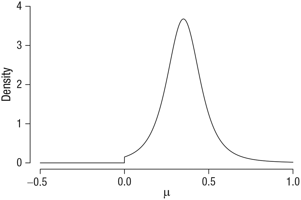
Example of an informed prior distribution for the overall effect size m: A t distribution with location 0.35, scale 0.102, and 3 df, truncated below at zero. This “Oosterwijk” prior (Gronau et al., 2020) will be used later in the example. Available at https://tinyurl.com/ycc965f2 under CC license https://creativecommons.org/licenses/by/2.0/.

^aOther effect size measures are, of course, possible and can be easily analyzed using the referenced software. Nevertheless, the parameter prior distributions need to be adjusted for other effect size measures.

Limitations of the random-effects model

Existing Bayesian meta-analysis procedures often focus on estimating the model parameters m and t of the random-effects model (T. C. Smith et al., 1995; Stangl & Berry, 2000). Specifically, they focus on interpreting the posterior distribution and possibly summaries of the posterior distribution such as the mean, median, or 95% CI. However, simply fitting a random-effects model assumes that both m and t are nonzero—implying that there is an effect and heterogeneity in the effect across studies—and then focuses on estimating the size of m and t. Nevertheless, it has been argued that before one estimates a parameter, one should test whether there is anything to be estimated (i.e., testing whether a parameter is equal to zero should precede parameter estimation; Fisher, 1928, p. 274; Haaf et al., 2019; Jeffreys, 1939, p. 345). Consequently, before estimating the parameters m and t, one should address, in a principled manner, two questions:

• Question 1 (Q1): Is the overall effect nonzero?

• Question 2 (Q2): Is there between-study variability in effect size?

Below we outline how to address these questions using Bayesian hypothesis testing in combination with Bayesian model averaging. ³ We have applied this framework to analyze power posing studies (Gronau, van Erp, et al., 2017), to investigate the effectiveness of descriptive social norms in facilitating ecological behavior (Scheibehenne et al., 2017), to test the compensatory control theory (Hoogeveen et al., 2018), to analyze facial feedback replication studies (Hinne et al., 2019), to analyze how research results are influenced by subjective decisions that scientists make as they design studies (Landy et al., 2020), and to reanalyze the Many Labs 4 data (Haaf et al., 2020). Furthermore, we have applied this methodology to analyze a set of replication studies concerning the ego depletion effect (Vohs et al., in press).

Four rival hypotheses

Our Bayesian model-averaged meta-analysis framework considers four candidate hypotheses (e.g., Gronau, van Erp, et al., 2017; Scheibehenne et al., 2017). ⁴ These correspond to the four possibilities for fixing to zero either m or t, both, or neither:

1. the fixed-effect null hypothesis ${\mathrm{\mathscr{H}}}_0^f$ : $\mathrm{\mu }=0$ , $\mathrm{\tau }=0$ ;

2. the fixed-effect alternative hypothesis ${\mathrm{\mathscr{H}}}_1^f$ : $\mathrm{\mu }\sim g(\cdot )$ , $\mathrm{\tau }=0$ ;

3. the random-effects null hypothesis ${\mathrm{\mathscr{H}}}_0^r$ : $\mathrm{\mu }=0$ , $\mathrm{\tau }\sim h(\cdot )$ ;

4. the random-effects alternative hypothesis ${\mathrm{\mathscr{H}}}_1^r$ : $\mathrm{\mu }\sim g(\cdot )$ , $\mathrm{\tau }\sim h(\cdot )$ .

Figure 3 displays the differences in prior specification for the four hypotheses (each hypothesis corresponds to a separate row). ⁵ Specifically, the first column displays the prior on the overall effect size m, and the second column displays the prior on the between-study standard deviation t. For the hypotheses in which the prior is not a point mass at zero, we have used the default prior recommendations from Box 1 (i.e., a zero-centered Cauchy prior with scale $1/\sqrt{2}$ on m and an Inverse-Gamma [1, 0.15] prior on t). The third column displays the implied joint prior on two hypothetical latent true study effects, ${\mathrm{\theta }}_i$ and ${\mathrm{\theta }}_j$ . ⁶ The fixed-effect null hypothesis ${\mathrm{\mathscr{H}}}_0^f$ fixes m and t to zero (Fig. 3, Row 1, Columns 1 and 2). Consequently, the true latent study effect is exactly zero for each study (Fig. 3, Row 1, Column 3). The fixed-effect alternative hypothesis ${\mathrm{\mathscr{H}}}_1^f$ fixes t to zero (Fig. 3, Row 2, Column 2) but allows m to differ from zero (i.e., m is assigned a continuous prior distribution; Fig. 3, Row 2, Column 1). Consequently, the latent true study effects can differ from zero. However, because ${\mathrm{\mathscr{H}}}_1^f$ does not specify any between-study variability (i.e., $\mathrm{\tau }=0$ ), all studies have the identical latent true effect size. Hence, the implied joint prior on two latent true study effects ${\mathrm{\theta }}_i$ and ${\mathrm{\theta }}_j$ assigns nonzero probability mass only to the diagonal line where ${\mathrm{\theta }}_i$ and ${\mathrm{\theta }}_j$ are identical (Fig. 3, Row 2, Column 3). The random-effects null hypothesis ${\mathrm{\mathscr{H}}}_0^r$ fixes the overall effect size m to zero (Fig. 2, Row 3, Column 1) but allows the between-study standard deviation t to differ from zero (i.e., t is assigned a continuous prior distribution; Fig. 3, Row 3, Column 2). Consequently, the latent true study effects may be different, but their distribution is centered on zero because the overall effect size m is fixed to zero (Fig. 3, Row 3, Column 3). Finally, the random-effects alternative hypothesis ${\mathrm{\mathscr{H}}}_1^r$ allows both m and t to differ from zero (Fig. 3, Row 4, Columns 1 and 2). Consequently, each latent true study effect is unique. The latent true study effects are correlated because their size depends on the specific values for m and t. Hence, a priori, one latent true study effect being large implies that another one will likely also be large. The distribution of two hypothetical latent true study effects is still centered on zero because the prior on the overall effect m is centered on zero. However, the prior under ${\mathrm{\mathscr{H}}}_1^r$ spreads out its mass across a larger range of effect size values than the prior under ${\mathrm{\mathscr{H}}}_0^r$ because m is assigned a continuous prior that allows values other than zero.

Fig. 3.

Parameter prior specifications for the four hypotheses of interest. Each row corresponds to one hypothesis (i.e., the fixed-effect null hypothesis [ ${\mathrm{\mathscr{H}}}_0^f]$ , the fixed-effect alternative hypothesis [ ${\mathrm{\mathscr{H}}}_1^f]$ , the random-effects null hypothesis $[{\mathrm{\mathscr{H}}}_0^r]$ , and the random-effects alternative hypothesis [ ${\mathrm{\mathscr{H}}}_1^r]$ ). The first column displays the prior distribution on the overall effect size m, and the second column displays the prior distribution on the between-study standard deviation t. For the hypotheses for which the prior is not a point mass at zero, we have used the default prior recommendations from Box 1 (i.e., a zero-centered Cauchy prior with scale $1/\sqrt{2}$ on m and an Inverse-Gamma[1, 0.15] prior on t). The third column displays the implied joint prior on two hypothetical latent true study effects, θ _i and θ _j . For the random-effects hypotheses, the contours reflect 5%, 25%, 50%, 75%, and 95% of probability within the area. Available at https://tinyurl.com/y98wqg5t under CC license https://creativecommons.org/licenses/by/2.0/.

Bayesian hypothesis testing

Each of the four rival hypotheses corresponds to one possible combination of the effect being present or absent and heterogeneity being present or absent. The goal is to assess the evidence for each of the four hypotheses by updating their plausibility according to the observed data. Given the shift in plausibility, one can then address Q1 and Q2 in a principled manner.

In the Bayesian framework, evidence for a model relative to another model is quantified using the Bayes factor (BF; Etz & Wagenmakers, 2017; Jeffreys, 1935, 1961; Kass & Raftery, 1995; Wrinch & Jeffreys, 1921). For example, one may be interested in the evidence for the fixed-effect model with an effect as opposed to the fixed-effect model with zero effect. The BF between these two models is

$$\underset{\begin{array}{c}\mathrm{BF}\\ \mathrm{for}\mathrm{effect}\end{array}}{\underbrace{{\mathrm{BF}}_{{\mathrm{\mathscr{H}}}_1^f,{\mathrm{\mathscr{H}}}_0^f}}}=\underset{\begin{array}{c}\mathrm{Relative}\mathrm{predictive}\\ \mathrm{accuracy}\end{array}}{\underbrace{\frac{p(\mathrm{data}|{\mathrm{\mathscr{H}}}_1^f)}{p(\mathrm{data}|{\mathrm{\mathscr{H}}}_0^f)}}},$$

(2)

in which $p(data|\mathrm{\mathscr{H}})$ denotes how well a hypothesis ℋ predicted the data at hand. Therefore, the BF may be interpreted as the relative predictive accuracy of two models (Rouder & Morey, 2019).

Here, we focus on an additional interpretation of the BF that comes from rearranging the terms of Bayes rule. According to the additional interpretation, the BF quantifies the change in beliefs about the hypotheses brought about by the data (i.e., the change from prior to posterior odds of two hypotheses):

$$\underset{\begin{array}{c}\mathrm{BF}\\ \mathrm{for}\mathrm{effect}\end{array}}{\underbrace{{\mathrm{BF}}_{{\mathrm{\mathscr{H}}}_1^f,{\mathrm{\mathscr{H}}}_0^f}}}=\underset{\begin{array}{c}\mathrm{Posterior}\mathrm{odds}\\ \mathrm{for}\mathrm{effect}\end{array}}{\underbrace{\frac{p({\mathrm{\mathscr{H}}}_1^f|\mathrm{data})}{p({\mathrm{\mathscr{H}}}_0^f|\mathrm{data})}}}/\underset{\begin{array}{c}\mathrm{Prior}\mathrm{odds}\\ \mathrm{for}\mathrm{effect}\end{array}}{\underbrace{\frac{p({\mathrm{\mathscr{H}}}_1^f)}{p({\mathrm{\mathscr{H}}}_0^f)}}}.$$

(3)

In this equation, $p({\mathrm{\mathscr{H}}}_1^f)$ denotes the prior probability of the fixed-effect alternative hypothesis ${\mathrm{\mathscr{H}}}_1^f$ , and $p({\mathrm{\mathscr{H}}}_1^f|data)$ denotes the posterior probability of ${\mathrm{\mathscr{H}}}_1^f$ (i.e., after having updated one’s knowledge according to observed data). Likewise, $p({\mathrm{\mathscr{H}}}_0^f)$ denotes the prior probability of the fixed-effect null hypothesis ${\mathrm{\mathscr{H}}}_0^f$ , and $p({\mathrm{\mathscr{H}}}_0^f|data)$ denotes the posterior probability of ${\mathrm{\mathscr{H}}}_0^f$ . ⁷

To illustrate how to quantify change in beliefs using the BF, we consider a hypothetical example. Figure 4 displays hypothetical prior and posterior probabilities for the four rival hypotheses. The top part of the plot shows prior probabilities of the hypotheses (i.e., plausibility before having seen any data), and by default, all of them are set to 0.25. The bottom panel of Figure 4 displays hypothetical posterior probabilities of the hypotheses (i.e., plausibility after having updated one’s knowledge according to observed data). In contrast to the prior probabilities, these are not equal anymore because the data have shifted one’s beliefs.

Fig. 4.

Prior probabilities of the hypotheses and computation of the model-averaged prior inclusion odds (top) and exemplary posterior probabilities and computation of the model-averaged posterior inclusion odds (bottom). Available at https://www.bayesianspectacles.org/library/ under CC license https://creativecommons.org/licenses/by/2.0/.

We are now ready to calculate the BF from Equation 3. For the hypothetical example in Figure 4, the prior odds are given by 0.25 / 0.25 = 1, and the posterior odds are given by 0.40 / 0.15 ≈ 2.67. Consequently, the BF is $B{F}_{{\mathrm{\mathscr{H}}}_1^f,{\mathrm{\mathscr{H}}}_0^f}\approx 2.67/1=2.67,$ which indicates that—assuming a fixed-effect model—the data have made the effect-present hypothesis 2.7 times more likely than it was before compared with the effect-absent hypothesis. In a similar fashion, one could compute $B{F}_{{\mathrm{\mathscr{H}}}_1^r,{\mathrm{\mathscr{H}}}_0^r}$ to quantify the evidence for the effect being nonzero assuming random effects. The prior odds are again given by $0.25/0.25=1$ , and the posterior odds are given by $0.35/0.10=3.5$ . Consequently, the BF is $B{F}_{{\mathrm{\mathscr{H}}}_1^r,{\mathrm{\mathscr{H}}}_0^r}=3.5/1$  = 3.5, which indicates that—assuming a random-effects model—the data have made the effect-present hypothesis 3.5 times more likely than it was before compared with the effect-absent hypothesis.

To address the question of whether there is heterogeneity in the effect across studies (Q2; i.e., test for fixed effect or random effects), one may compute $B{F}_{{\mathrm{\mathscr{H}}}_1^r,{\mathrm{\mathscr{H}}}_1^f}$ . This BF compares the random-effects hypothesis with the fixed-effect hypothesis under the assumption that effect size m is nonzero. For the hypothetical example in Figure 4, the prior odds are given by $0.25/0.25=1$ , and the posterior odds are given by $0.35/0.40=0.875$ . Consequently, $B{F}_{{\mathrm{\mathscr{H}}}_1^r,{\mathrm{\mathscr{H}}}_1^f}=(0.35/0.40)/1=0.875$ or, equivalently, $B{F}_{{\mathrm{\mathscr{H}}}_1^f,{\mathrm{\mathscr{H}}}_1^r}=1/B{F}_{{\mathrm{\mathscr{H}}}_1^r,{\mathrm{\mathscr{H}}}_1^f}\approx 1.14$ . This BF indicates that—assuming that an effect is present—the data have made the heterogeneity-absent hypothesis about 1.14 times more likely than it was before, compared with the heterogeneity-present hypothesis.

Bayesian model averaging

For the fictional scenario above, one could conclude that the BF in favor of the effect-present hypothesis is either $B{F}_{{\mathrm{\mathscr{H}}}_1^r,{\mathrm{\mathscr{H}}}_0^r}=3.5$ (if there is heterogeneity in the effect) or $B{F}_{{\mathrm{\mathscr{H}}}_1^f,{\mathrm{\mathscr{H}}}_0^f}$ ≈ 2.67 (if there is no heterogeneity). Furthermore, the data support both the random-effects alternative hypothesis and the fixed-effect alternative hypothesis about equally (i.e., assuming an effect, $B{F}_{{\mathrm{\mathscr{H}}}_1^f,{\mathrm{\mathscr{H}}}_1^r}$ ≈ 1.14). Hence, considerable uncertainty remains with respect to whether a fixed-effect or a random-effects model is more appropriate. Instead of ignoring this uncertainty for final inference, one can take this uncertainty into account by considering all four hypotheses simultaneously according to their plausibility in light of the observed data. This procedure is known as Bayesian model averaging (e.g., Hinne et al., 2019; Hoeting et al., 1999).

To quantify the evidence for the effect being present while taking into account uncertainty with respect to choosing a fixed-effect or random-effects model, one can compute a model-averaged inclusion BF. This BF contrasts all hypotheses that allow the effect to be nonzero (i.e., ${\mathrm{\mathscr{H}}}_1^f$ and ${\mathrm{\mathscr{H}}}_1^r$ ) to all hypotheses that constrain the effect to be exactly zero (i.e., ${\mathrm{\mathscr{H}}}_0^f$ and ${\mathrm{\mathscr{H}}}_0^r$ ) and thus fully takes into account model uncertainty with respect to choosing a fixed-effect or random-effects model. ⁸ Figure 4 illustrates how this model-averaged inclusion BF is computed. This BF, just as any BF, is given by the change from prior to posterior odds. However, this time, these are prior and posterior inclusion odds. The top panel of Figure 4 displays the prior probabilities of the hypotheses. By default, all of them are set to 0.25. The left scale shows how to compute the prior inclusion odds for the presence of an effect. Specifically, the hypotheses that allow m to differ from zero (i.e., ${\mathrm{\mathscr{H}}}_1^r$ and ${\mathrm{\mathscr{H}}}_1^f$ ) are contrasted with the hypotheses that fix m to zero (i.e., ${\mathrm{\mathscr{H}}}_0^r$ and ${\mathrm{\mathscr{H}}}_0^f$ ). Because the combined prior probability of the hypotheses that allow m to differ from zero is 0.50 and the combined prior probability of the hypotheses that fix m to zero is also 0.50, the prior inclusion odds are equal to 1. ⁹ The bottom panel of Figure 4 illustrates how to compute the posterior inclusion odds using hypothetical posterior probabilities. In contrast to the prior probabilities, these are not equal anymore after having updated one’s knowledge according to observed data. The left scale in Figure 4 compares the hypotheses that allow m to differ from zero with the hypotheses that fix m to zero. Given the posterior probabilities, this comparison favors the hypotheses that allow m to be nonzero (combined posterior probability of 0.75) over the hypotheses that fix m to zero (combined posterior probability of 0.25). Consequently, the posterior inclusion odds are given by 0.75 / 0.25 = 3. Finally, the model-averaged inclusion BF for an effect is obtained by dividing the posterior inclusion odds by the prior inclusion odds ¹⁰ :

$$\underset{\begin{array}{c}\mathrm{Inclusion}\mathrm{BF}\\ \mathrm{for}\mathrm{effect}\end{array}}{\underbrace{{\mathrm{BF}}_{10}}}=\underset{\begin{array}{c}\mathrm{Posterior}\mathrm{inclusion}\mathrm{odds}\\ \mathrm{for}\mathrm{effect}\end{array}}{\underbrace{\frac{p({\mathrm{\mathscr{H}}}_1^f|\mathrm{data})+p({\mathrm{\mathscr{H}}}_1^r|\mathrm{data})}{p({\mathrm{\mathscr{H}}}_0^f|\mathrm{data})+p({\mathrm{\mathscr{H}}}_0^r|\mathrm{data})}}}/\underset{\begin{array}{c}\mathrm{Prior}\mathrm{inclusion}\mathrm{odds}\\ \mathrm{for}\mathrm{effect}\end{array}}{\underbrace{\frac{p({\mathrm{\mathscr{H}}}_1^f)+p({\mathrm{\mathscr{H}}}_1^r)}{p({\mathrm{\mathscr{H}}}_0^f)+p({\mathrm{\mathscr{H}}}_0^r)}}}.$$

(4)

In this example, dividing the posterior inclusion odds by the prior inclusion odds yields $B{F}_{10}=3/1=3$ . This BF indicates that compared with the effect-absent hypothesis, the data have made the effect-present hypothesis 3 times more likely than it was before.

In a similar fashion, one can compute a model-averaged inclusion BF to compare all hypotheses that allow the between-study standard deviation τ to be nonzero (i.e., ${\mathrm{\mathscr{H}}}_0^r$ and ${\mathrm{\mathscr{H}}}_1^r$ ) to all hypotheses that fix τ to zero (i.e., ${\mathrm{\mathscr{H}}}_0^f$ and ${\mathrm{\mathscr{H}}}_1^f$ ):

$$\underset{\begin{array}{c}\mathrm{Inclusion}\mathrm{BF}\\ \mathrm{for}\mathrm{heterogeneity}\end{array}}{\underbrace{{\mathrm{BF}}_{rf}}}=\underset{\begin{array}{c}\mathrm{Posterior}\mathrm{inclusion}\mathrm{odds}\\ \mathrm{for}\mathrm{heterogeneity}\end{array}}{\underbrace{\frac{p({\mathrm{\mathscr{H}}}_0^r|\mathrm{data})+p({\mathrm{\mathscr{H}}}_1^r|\mathrm{data})}{p({\mathrm{\mathscr{H}}}_0^f|\mathrm{data})+p({\mathrm{\mathscr{H}}}_1^f|\mathrm{data})}}}/\underset{\begin{array}{c}\mathrm{Prior}\mathrm{inclusion}\mathrm{odds}\\ \mathrm{for}\mathrm{heterogeneity}\end{array}}{\underbrace{\frac{p({\mathrm{\mathscr{H}}}_0^r)+p({\mathrm{\mathscr{H}}}_1^r)}{p({\mathrm{\mathscr{H}}}_0^f)+p({\mathrm{\mathscr{H}}}_1^f)}}}.$$

(5)

The computation of this BF is also illustrated in Figure 4 (i.e., scales on the right). The prior inclusion odds for heterogeneity are equal to 1, and the posterior inclusion odds are equal to 0.45/0.55 ≈ 0.82. Consequently, $B{F}_{rf}=(0.45/0.55)/1\approx 0.82$ , or expressed in favor of no heterogeneity, $B{F}_{fr}$ ≈ 1.22. This BF indicates that compared with the heterogeneity-present hypothesis, the data have made the heterogeneity-absent hypothesis about 1.22 times more likely than it was before.

One may also use model averaging in estimation to obtain a model-averaged posterior distribution for the parameters m and t. These model-averaged posterior distributions combine the posterior for each hypothesis by weighting them with the posterior probability of each hypothesis. There are two useful ways of obtaining model-averaged posteriors. First, one may combine the posterior for, say, m for all four hypotheses according to their posterior probabilities. Because two of the hypotheses fix m a priori to zero (i.e., ${\mathrm{\mathscr{H}}}_0^f$ and ${\mathrm{\mathscr{H}}}_0^r$ ), the model-averaged posterior will be a mixture between a point-mass at zero and a continuous component. Second, one could choose to focus only on the hypotheses that do not fix the parameter to zero. This yields a model-averaged posterior without a spike at zero. Importantly, in this case, one needs to be clear about the fact that this represents the model-averaged posterior under the assumption that the effect is nonzero. In the software that we use below (i.e., metaBMA and JASP), only the latter approach has currently been implemented (i.e., displaying the model-averaged posterior conditional on assuming that the effect is present).

Example: Testing the Self-Concept Maintenance Theory

According to the self-concept maintenance theory (Mazar et al., 2008), people will cheat to maximize self-profit, but only to the extent that they can still maintain a positive self-view. In their Experiment 1, Mazar et al. (2008) gave participants an incentive and opportunity to cheat. Before working on a problem-solving task, participants either recalled, as a moral reminder, the Ten Commandments or, as a neutral condition, 10 books they had read in high school. In line with the self-concept maintenance hypothesis, participants in the moral reminder condition reported having solved fewer problems than those in the neutral condition, which also reflected their actual performance better. Recently, a Registered Replication Report (Verschuere et al., 2018) attempted to replicate this finding. Here we focus on the primary meta-analysis that included data from 19 labs. Figure 5 displays the observed Cohen’s d effect size and corresponding 95% CI for each lab. ¹¹ Negative effect sizes are in line with the self-concept maintenance hypothesis (i.e., the self-concept maintenance theory predicts that participants in the Ten Commandments condition cheat less than participants in the neutral condition, not more), whereas positive effect sizes are opposite to what the theory predicts.

Fig. 5.

Observed effect sizes (Cohen’s d) with corresponding 95% confidence intervals for the Registered Replication Report by Verschuere et al. (2018). Only the 19 labs that were included in the primary analysis are displayed. Available at https://tinyurl.com/ydad5k7p under CC license https://creativecommons.org/licenses/by/2.0/.

For the primary analysis, Verschuere et al. (2018) reported a meta-analytic Cohen’s d of 0.04 (95% CI = [−0.04, 0.12]). ¹² Consequently, the effect was nonsignificant and in the opposite direction of the effect size in the original study. Furthermore, Verschuere et al. concluded that there was no heterogeneity across labs: ${\mathrm{\tau }}^2=0$ , $Q(18)=13.16$ , $p=.78$ . Here we conduct a reanalysis using the Bayesian model-averaged meta-analysis approach.

Parameter prior settings

We use three different parameter prior specifications. These specifications differ only in the prior for m because the prior for t is always an Inverse-Gamma(1, 0.15) distribution. The first specification assigns m a default zero-centered Cauchy prior distribution with scale $1/\sqrt{2}$ . This specification will be referred to as default (two-sided). The second specification is very similar but truncates the default Cauchy prior distribution at zero to incorporate the directedness of the self-concept maintenance hypothesis (i.e., participants in the Ten Commandments condition are expected to cheat less than participants in the neutral condition, not more). This specification will be referred to as default (one-sided). Finally, the third specification uses as an informed prior for m a t distribution that is centered on −0.35, with scale 0.102 and 3 df. This prior is also truncated at zero to preclude effect sizes in the direction opposite to what the hypothesis predicts. This “Oosterwijk” prior has been elicited for a reanalysis of a social psychology study (Gronau et al., 2020), but we believe it is a reasonable prior for psychological studies more generally. ¹³ This specification will be referred to as informed (one-sided).

Results

Hypotheses posterior probabilities

Table 1 displays the prior and posterior probabilities of the hypotheses for each of the three different prior specifications. The ordering of the posterior probabilities is identical for all three prior specifications: The fixed-effect null hypothesis ( ${\mathrm{\mathscr{H}}}_0^f)$ receives most posterior probability, followed by the random-effects null hypothesis $({\mathrm{\mathscr{H}}}_0^r)$ , the fixed-effect alternative hypothesis $({\mathrm{\mathscr{H}}}_1^f)$ , and the random-effects alternative hypothesis $({\mathrm{\mathscr{H}}}_1^r)$ .

Table 1.

Prior and Posterior Probabilities of the Four Hypotheses of Interest

Hypothesis	p(ℋ)	$p(\mathrm{\mathscr{H}}|\mathrm{data})$
		Default (two-sided)	Default (one-sided)	Informed (one-sided)
${\mathrm{\mathscr{H}}}_0^f$	0.25	0.754	0.823	0.837
${\mathrm{\mathscr{H}}}_1^f$	0.25	0.087	0.017	0.004
${\mathrm{\mathscr{H}}}_0^r$	0.25	0.143	0.156	0.159
${\mathrm{\mathscr{H}}}_1^r$	0.25	0.016	0.004	0.001

Note: Data from Verschuere et al. (2018). ${\mathrm{\mathscr{H}}}_0^f$ = fixed-effect null hypothesis; ${\mathrm{\mathscr{H}}}_1^f=$ fixed-effect alternative hypothesis; ${\mathrm{\mathscr{H}}}_0^r$ = random-effects null hypothesis; ${\mathrm{\mathscr{H}}}_1^r$ = random-effects alternative hypothesis.

Model-averaged BF for an overall effect

To address the question of whether the meta-analytic effect is nonzero (i.e., Q1), we compute the model-averaged BF, BF₁₀, for each prior setting. This can be achieved solely using the probabilities presented in Table 1. For the default (two-sided) prior setting, the posterior inclusion odds for an effect are given by $(0.087+0.016)/(0.754+0.143)\approx 0.115$ . Because the prior inclusion odds are equal to 1, this number equals the model-averaged BF, BF₁₀ ≈ 0.115. Consequently, $B{F}_{01}=1/B{F}_{10}\approx 8.696$ , which indicates moderate evidence for the absence of an effect. For the default (one-sided) prior setting, the posterior inclusion odds for an effect are given by $(0.017+0.004)/(0.823+0.156)\approx 0.021$ ; this number equals the model-averaged BF, BF₁₀ ≈ 0.021. Consequently, $B{F}_{01}=1/B{F}_{10}\approx 47.619$ , which indicates very strong evidence for the absence of an effect. For the informed (one-sided) prior setting, the posterior inclusion odds are calculated in the same fashion. The model-averaged BF is therefore $B{F}_{10}\approx (0.004+0.001)/(0.837+0.159)\approx$ . Consequently, $B{F}_{01}=1/B{F}_{10}\approx 200$ , which indicates extreme evidence for the absence of an effect. In sum, for all prior settings, the model-averaged BF indicates evidence in favor of the null hypothesis of no effect. However, the degree of evidence differs across prior settings. The reason why the default (one-sided) and the informed (one-sided) prior setting yield more evidence for the absence of an effect is that, as reported by Verschuere et al. (2018), the meta-analytic effect goes in the direction opposite of what the theory predicts, and these priors for m do not assign any mass to population effect size values that go in the opposite direction.

Model-averaged BF for heterogeneity

To address the question of whether there is heterogeneity in effect size across studies (i.e., Q2), we compute the model-averaged BF, BF_rf, for each prior setting. This can again be achieved solely using the probabilities presented in Table 1. For the default (two-sided) prior setting, the posterior inclusion odds for heterogeneity are given by $(0.143+0.016)/(0.754+0.087)\approx 0.189$ . Because the prior inclusion odds are equal to 1, this number equals the model-averaged BF, BF_rf ≈ 0.189. Consequently, $B{F}_{fr}=1/B{F}_{rf}\approx 5.291$ , which indicates moderate evidence for the absence of heterogeneity. For the default (one-sided) prior setting, the posterior inclusion odds for heterogeneity are given by $(0.156+0.004)/(0.823+0.017)\approx 0.190$ ; this number equals the model-averaged BF, BF_rf ≈ 0.190. Consequently, $B{F}_{fr}=1/B{F}_{rf}\approx 5.263$ , which indicates moderate evidence for the absence of heterogeneity. For the informed (one-sided) prior setting, the model-averaged BF is given by $B{F}_{rf}\approx (0.159+0.001)/(0.837+0.004)\approx 0.190$ . Consequently, $B{F}_{fr}=1/B{F}_{rf}\approx 5.263$ , which indicates moderate evidence for the absence of heterogeneity. In sum, for all prior settings, the model-averaged BF indicates evidence in favor of the null hypothesis of no heterogeneity. The degree of evidence is very similar across prior settings, which indicates moderate evidence for the absence of heterogeneity.

Sequential analysis

For this particular example, studies were conducted at about the same time, and we do not know the order in which they finished. However, in other cases, the temporal order may be known and of interest. This is especially the case for meta-analyses combining studies from several decades because trends in the field may affect study design and results. Here we demonstrate how to conduct a sequential analysis that displays the evidence as studies accumulate. Because the presented approach is Bayesian, current knowledge can be updated by new evidence without having to worry about optional stopping (Rouder, 2014). To demonstrate the sequential analysis, we make the arbitrary assumption that the temporal order of the studies coincides with the alphabetical order of the last names of the labs’ leading researchers. Furthermore, for demonstration purposes, we focus on one prior setting, default (two-sided). Figure 6 displays how the posterior probability for each of the four hypotheses changes as studies accumulate. Note that at the zero point of the x-axis, all hypotheses have “posterior” probability 0.25: Without any data, the posterior probability equals the prior probability. Figure 6 highlights that the posterior probability for the fixed-effect null hypothesis, ${\mathrm{\mathscr{H}}}_0^f,$ increases as more studies become available. Compared with the prior probability, all other hypotheses decrease in plausibility over time. Note that both hypotheses that fix effect size m to zero ( ${\mathrm{\mathscr{H}}}_0^f$ and ${\mathrm{\mathscr{H}}}_0^r$ ) have a higher posterior probability than the two hypotheses that allow m to differ from zero ( ${\mathrm{\mathscr{H}}}_1^f$ and ${\mathrm{\mathscr{H}}}_1^r$ ). The lines end with the inclusion of Study 19, and this point describes the current state of evidence. However, as more studies become available, one could extend this analysis further and interpret the updated state of evidence (Berger & Wolpert, 1988; Rouder, 2014; Wagenmakers, Gronau, & Vandekerckhove, 2018).

Fig. 6.

Sequential analysis. The posterior probability for each of the four hypotheses is displayed as a function of the number of studies included in the analysis. Figure from JASP (jasp-stats.org).

Parameter posterior distribution

As shown above, all prior settings resulted in evidence against the self-concept maintenance theory. It could be argued that this makes estimation of the population effect size unnecessary—the data offer no reason to consider an estimate other than $\mathrm{\mu }=0$ . Nevertheless, in practice, it may still be of interest to show how small or large the effect size is estimated under the assumption that the effect is nonzero. In general, we believe that for parameter estimation, it is advisable to not use a truncated prior for the parameter of interest (van Doorn et al., 2019). The reason is that, as in the present example, the effect may be in the direction opposite to what the hypothesis predicts. Whenever a prior is truncated to allow only effect sizes that align with the hypothesis, it is impossible to obtain a posterior that assigns probability mass to effect sizes in the opposite direction. As a consequence, a posterior distribution based on truncated priors may be misleading (in the present example, the truncated posterior would be left-skewed with almost all probability mass close to zero). Figure 7 displays the posterior distribution for m using the default (two-sided) prior setting. Posteriors are shown for both hypotheses that allow m to differ from zero ( ${\mathrm{\mathscr{H}}}_1^f$ and ${\mathrm{\mathscr{H}}}_1^r$ ) and, additionally, the model-averaged posterior that is obtained by combining these two posteriors according to the plausibility of the hypotheses according to the data. Figure 7 shows that, assuming m is not exactly equal to zero, it is likely to be small and have most posterior mass in the direction opposite to what the theory predicts. Furthermore, the posterior distributions under both hypotheses are very similar, which results in a model-averaged posterior that is also very similar.

Fig. 7.

Posterior distribution for the effect size parameter m. The posterior is displayed for both hypotheses that do not fix m to zero. In addition, the model-averaged posterior distribution is displayed. The prior distribution is shown as a dotted line. Figure from JASP (jasp-stats.org).

Discussion

In this primer, we have discussed Bayesian model-averaged meta-analysis as a method for quantitatively synthesizing the results of a set of studies. This procedure affords researchers the well-known pragmatic benefits of a Bayesian method (Wagenmakers, Marsman, et al., 2018; Wagenmakers, Morey, & Lee, 2016). In addition, it allows researchers to take into account model uncertainty with respect to choosing a fixed-effect or random-effects model when addressing the two key questions of whether the overall effect is nonzero (Q1) and whether there is between-study variability in effect size (Q2).

Effects of prior settings

There are two a priori settings to consider for a Bayesian model-averaged meta-analysis: the prior probabilities for the four models (i.e., prior model probabilities) and the prior distributions for the overall effect m and the study heterogeneity t (i.e., prior parameter distributions). We now discuss each setting in turn.

Concerning the prior model probabilities, in the Appendix we show how the results change as a function of how the prior probability is distributed across the four models. When comparing two models, the choice of prior model probabilities does not affect the BF; however, this is no longer the case when more than two models are in play. In such scenarios, the model-averaged BFs are generally sensitive to the choice of prior model probabilities. For unequal prior probabilities, the posterior probabilities may change quite drastically. In our application to the data from Verschuere et al. (2018), however, the pattern of BF is relatively robust to reasonable changes in the prior model probabilities (see Appendix). Nevertheless, we recommend using uniform prior probability settings across the models if there are no clear theoretical reasons for different settings.

Concerning the prior distributions for the model parameters, concrete recommendations are provided in Box 1. We showed that in our application to the data from Verschuere et al. (2018), for some reasonably informed choices, the pattern of evidence from the BFs is comparable. The more informed a prior distribution is (e.g., choosing a one-sided prior distribution for the overall effect size), the faster evidence accumulates for or against this hypothesis. When in doubt about these settings, we recommend conducting a robustness analysis in which researchers choose several reasonable prior settings and check how these choices affect the results. Note that in this primer, we focused on standardized mean difference effect sizes (i.e., Cohen’s d or Hedges’s g) and provided recommendations for how to choose the prior distributions for this case. If the observed effect sizes are not standardized mean differences, one needs to adjust these prior distributions. Providing recommendations for other cases such as Fisher’s z and log odd ratios is left to future research.

Justification of the models

Up to this point, we have tacitly assumed that each of the four models under consideration is a reasonable abstraction of a possible real-world phenomenon that a researcher is interested in. We do not believe that any of the models are “true” in the sense that they correspond to reality exactly. As stated by A. F. M. Smith (1981),

as soon as we make any selection from the huge complex of assumptions (i.e. models) available to us, we are entering into a kind of metaphor. All models are metaphors. We must always recognize that underlying everything we do is an “as if” philosophy. We should always be saying (as loudly as possible) “I am going to condition on certain assumptions, and anything I say has to be interpreted as if (at this moment) I believe in those assumptions.” (p. 121)

Nevertheless, the usefulness of some of the models in our set may be disputed. This holds particularly for the fixed-effect models, which assume that the true effect size is identical across all studies, and the random-effects null hypothesis, which assumes that each experiment has a nonzero effect but that the group mean equals zero exactly. We will discuss these models in turn.

Fixed-effect models

Some methodologists have argued that a parameter is never truly equal to zero (e.g., Bakan, 1966; Cohen, 1994; Laplace, 1774/1986; Meehl, 1967, 1978; Nunnally, 1960; Schmidt & Hunter, 1997; Tukey, 1991). From this perspective, the fixed-effect models are deemed utterly implausible from the outset because the between-studies variability t is assumed to equal zero exactly (but see Hedges & Vevea, 1998). ¹⁴ In line with the quotation from Adrian Smith (1981) above, our view is that all models are abstractions and should be interpreted as metaphors. Fixing t = 0 is an implementation of the theoretical position that between-study variability is negligible. Of course, with infinitely many studies, t may not be exactly zero. With a finite number of studies, however, the models that fix t to zero may outpredict the competition, particularly if the number of available studies is small. Random-effects models are less parsimonious and require more studies for their parameters to be estimated accurately. If between-study variability t is indeed nonzero, the plausibility of the fixed-effect models will wane as studies accumulate, and the plausibility of the random-effects models will wax. At any point, the relative influence of the fixed-effect as opposed to the random-effects models is a function of predictive performance: If the fixed-effect models indeed predict the observed data poorly, they will simply not receive much posterior probability, and model-averaged inference will be driven primarily by the random-effects models. Finally, the results produced by assuming a point-null hypothesis t = 0 will be similar to those produced by assuming a peri-null hypothesis that assigns t a distribution that is highly concentrated near zero. Researchers who are uncomfortable with point-null hypotheses may view them as mathematically convenient approximations to more realistic peri-null hypotheses that assume t to be negligibly small (but not equal to zero exactly). ¹⁵

Random-effects null hypothesis

Researchers who believe a parameter is never truly equal to zero may similarly object to the random-effects null hypothesis that fixes the group mean m to zero. In fact, for the case of the random-effects null hypothesis, there is an added concern: How could it be possible that each study effect itself is nonzero but the group mean of the study effects happens to average out to zero exactly? Even if the group mean were virtually zero at some stage, adding another study would almost certainly move it away from zero again. ¹⁶ We agree that these are valid objections. Nevertheless, we remain convinced that including this model in the model-averaging procedure is sound rather than silly. ¹⁷ As before, one may consider the random-effects null hypothesis as a mathematically convenient approximation of the peri-null hypothesis that states the effect is not exactly zero but falls in an interval close to zero. In other words, the model effectively assumes that any changes in the group mean are dwarfed by study-specific effects (e.g., due to unknown moderators). If this model were excluded, any systematic variation in effects across studies will greatly heighten the plausibility of the random-effects ${\mathrm{\mathscr{H}}}_1$ , which also states that there is an effect on the group mean. In other words, without the random-effects null hypothesis in the model set, a single experiment with a clear effect suffices to conclude that there exists an effect across all experiments as well. We believe that both skeptical and pragmatic researchers will find this conclusion premature. Thus, including the random-effects null hypothesis provides a check on the random-effects alternative hypothesis, dampens the impact of outlying experiments, and generally makes the inference more robust to model misspecification. Finally, if the random-effects null hypothesis truly provides a terrible account of the observed data, its posterior probability will be close to zero, and it will play a negligible role in the model-averaging procedure.

Caveats

There exist a number of caveats for both the proposed Bayesian meta-analysis approach specifically and meta-analysis in general. The main danger is that researchers treat the outcome of a meta-analysis as definitive without taking into account the assumptions and limitations of the approach. In general, there are many uncertainties when applying meta-analysis; the proposed approach attempts to address one of these uncertainties (i.e., should a fixed-effect or random-effects model be used) using Bayesian model averaging. One uncertainty that is not addressed by the approach is whether the assumption of a normal distribution of true study effects is plausible. It may be argued that this assumption is problematic because of a number of reasons. For example, there may be dependencies between different effect sizes due to including multiple effect sizes from the same articles or multiple studies from the same lab. Moreover, there may be sequential dependencies given that researchers may inform their study designs by reading the literature (this may be less of a concern for many-labs meta-analyses). Furthermore, researchers should be aware that there may be measurement-error and range-restriction issues. A number of methods have been proposed to address these caveats (e.g., Cheung & Chan, 2008; Schmidt & Hunter, 2015; Tipton, 2015). Another caveat is that the presence of publication bias may distort the meta-analytic result. Publication bias can be ruled out in case the complete set of studies has been preregistered (e.g., in the form of a Registered Replication Report, Chambers, 2017; van Elk et al., 2015). Whenever publication bias cannot be ruled out, a number of methods have been proposed for estimating the extent of this publication bias and for correcting the meta-analytic effect size estimate (e.g., Gronau, Duizer, et al., 2017; Simonsohn et al., 2014a, 2014b; van Assen et al., 2015). ¹⁸ Furthermore, our lab has recently proposed an extension of the Bayesian model-averaged meta-analysis procedure that takes into account the possibility of publication bias (Bartoš et al., 2020; Maier et al., 2020). In any case, it is important to emphasize that researchers should not blindly trust meta-analysis results but should take into account substantive expertise and knowledge about the limitations of the procedure.

Beyond overall effects

In addition to the key questions Q1 and Q2, researchers may often be interested in incorporating discrete and continuous moderators at the study level. Although we did not discuss this possibility here, the metaBMA package does provide functionality for including moderators. Including moderators in the analysis is one way of accounting for the fact that different subsets of studies might have different latent effect sizes. Another possible way of incorporating and testing this assumption would be to change the distribution of the latent study effects. Instead of assuming a single continuous normal distribution of effect sizes, one could assume a latent mixture of normal distributions and then test how many components are necessary to describe the distribution of latent study effects best (e.g., Moreau & Corballis, 2019).

An additional approach to a Bayesian meta-analysis is to focus on the entire distribution of study effects instead of the overall effect. For instance, Rouder et al. (2019) proposed to test whether all studies in the meta-analytic sample show an effect in the same, expected direction or whether some studies show an opposite effect. An appropriate model for this analysis is one in which both the distribution of the overall effect and the distribution of individual study effects are truncated; the latter truncation is imposed to allow individual study effects in one direction only (upper level of Fig. 1). This model can then be compared with the unconstrained alternative (i.e., the random-effects alternative). Similar tests have been proposed in the clinical literature, in which meta-analysis also serves the purpose to test whether one treatment is superior for one patient population and another treatment is superior for another patient population (Gail & Simon, 1985). Such a “Does every study show an effect?” analysis is implemented in the metaBMA package.

As a final word of caution, we would like to stress again that, in line with the adage “garbage in, garbage out,” no statistical analysis can provide high-quality inference based on low-quality data that might be the result of problematic study design, shortcomings of the implementation or sample, publication bias, significance chasing, and so on; Bayesian model-averaged meta-analysis is no exception. For instance, one may use the procedure to analyze studies that have not been preregistered; however, the conclusions might need to be interpreted with skepticism in case the quality of the included studies is questionable or if the included studies represent a biased sample of all conducted studies in a field. In contrast, when the set of studies is of high quality, preregistered, and possibly even the result of a Registered (Replication) Report, we believe that Bayesian model-averaged meta-analysis can be a valuable tool that allows researchers to address key questions of interest in a principled manner.