Sage Journals: Discover world-class research

Abstract

Psychological theories often invoke interactions but remain vague regarding the details. As a consequence, researchers may not know how to properly test them and may potentially run analyses that reliably return the wrong answer to their research question. We discuss three major issues regarding the prediction and interpretation of interactions. First, interactions can be removable in the sense that they appear or disappear depending on scaling decisions, with consequences for a variety of situations (e.g., binary or categorical outcomes, bounded scales with floor and ceiling effects). Second, interactions may be conceptualized as changes in slope or changes in correlations, and because these two phenomena do not necessarily coincide, researchers might draw wrong conclusions. Third, interactions may or may not be causally identified, and this determines which interpretations are valid. Researchers who remain unaware of these distinctions might accidentally analyze their data in a manner that returns the technically correct answer to the wrong question. We illustrate all issues with examples from psychology and issue recommendations for how to best address them in a productive manner.

Keywords

assumptions causality interaction measurement scale open materials

“Forty-two!” yelled Loonquawl. “Is that all you’ve got to show for seven and a half million years’ work?”

“I checked it very thoroughly,” said the computer, “and that quite definitely is the answer. I think the problem, to be quite honest with you, is that you’ve never actually known what the question is.”

“But it was the Great Question! The Ultimate Question of Life, the Universe and Everything,” howled Loonquawl.

—Douglas Adams, The Hitchhiker’s Guide to the Galaxy

Interactions are ubiquitous in psychological science. Person-situation interactions, stress-vulnerability models, gene-environment interactions—a large number of theoretical perspectives postulate that the effect of one variable depends on another variable. Interactions often seem highly plausible from a substantive perspective, and in many empirical investigations, they are considered the central target of inquiry. Thus, it is no surprise that statistical procedures to test for interactions are a standard part of psychologists’ toolkits. In experimental subfields, analysis of variance (ANOVA) is the favored approach: Group means are compared, and per default, statistical packages will include the interaction term and report its magnitude and statistical significance. In nonexperimental subfields, researchers frequently implement an equivalent multiple regression approach: The product between two or more variables is included as a predictor, and the resulting coefficient quantifies the interaction.

Establishing an interaction through these means might seem like a straightforward task; however, there is a range of potential complications. For one, reliably detecting interactions can be a challenge. There is some empirical evidence suggesting that interaction claims are less replicable (Beck & Jackson, 2020; Open Science Collaboration et al., 2015), and there are a priori reasons to expect so. To find interactions in which an effect is attenuated in one group but not reversed compared with the other group, surprisingly large sample sizes are needed (e.g., Gelman, 2018; Giner-Sorolla, 2018; Lakens, 2020). This means that existing interaction effects are harder to confirm in empirical studies—but also that reportedly significant interactions are more likely to be false positives or even point in the wrong direction. Furthermore, studies with experimental interventions might afford only one plausible main effect but many different interactions to be considered (e.g., intervention times any demographic variable assessed), leading to a large number of researcher degrees of freedom that may further increase the risk of false positives.

However, other issues with interactions can result in reliably mistaken conclusions. Rerunning the same study will not fix or reveal those issues—instead, one may get the wrong answer every time. Some of these issues can be identified by close investigation of the data alone. For example, Hainmueller et al. (2019) discussed two problems and how to address them: The standard approach to interaction assumes a linear interaction effect that can be a misspecification, and estimates can be misleading if there are little data underlying certain regions of values (e.g., if at some values of one of the interacting variables, there is little variability in the other interacting variable). But there is another set of issues that cannot be resolved by careful consideration of the data alone.

It is three such replicable issues with interactions on which we want to focus in the present article: the scale dependence of interactions, the distinction between moderation of slopes compared with moderation of correlation, and the causal identification of interactions. We work through each of these issues with a motivating example based on data that have been simulated (which ensure that we know the true model) followed by relevant examples from the literature.

All of these issues have been discussed before, sometimes in great detail and clarity, often within specific substantive contexts, and we highlight some of these works throughout the article. Yet a look at contemporary publications in psychological journals suggests that researchers with a substantive focus often do little to address them. They may have multiple reasons: (a) Researchers may not be aware of them, or (b) they may consider them esoteric details without consequences for their own substantive conclusions, or (c) they simply may not know how to address them best. Thus, in the present article, we aim to (a) clearly explain these problems using simulated data, (b) illustrate how they can indeed affect substantive conclusions in published research, and (c) provide constructive recommendations on how to address them. In passing, we demonstrate that each of the three issues with interactions points to a broader problem that also affects claims about main effects.

Now You See It, Now You Don’t: Interactions Are Scale Dependent

Motivating example

A large company is testing a mentoring program with the hope of increasing employee retention. For this purpose, 10% of employees have been randomly assigned to participate in the program, and the company plans to evaluate its effects on quitting 1 year later. But then a global pandemic forces a change of plan, and because of distancing measures, only half of the employees can work on site, with the other half working remotely. The decision who still works on site has been randomized. All the while, the mentoring program is continued through video conferencing.

Once the time has come for the evaluation of the mentoring program, there are now two questions that can be evaluated: Did the mentoring program reduce quitting? And did it do so equally for on-site and remote workers—in other words, was there an interaction between the mentoring program and work location?

All models reported in this article have been estimated in brms (Bürkner, 2017, 2018) using default, weakly informative priors. Note that all the problems discussed in this article occur regardless of whether a frequentist or a Bayesian approach is chosen and whether an ANOVA or a regression is run; however, brms as a highly flexible statistical package allows us to adapt the models and procedures to easily mitigate the problems discussed here. Table 1 shows results from a logistic regression on simulated data in which the binary outcome quitting (0 = no, 1 = yes) was regressed onto three predictors: mentoring program participation (0 = no, 1 = yes), working on site (0 = no [remote work], 1 = yes), and the product term of the two (Mentoring × Working on Site interaction).

Table 1.

Results From a Logistic Regression Analysis Predicting Quitting From Participation in the Mentoring Program, Working on Site, and Their Interaction

Variable	Coefficient	95% CI
Intercept	−3.06	[−3.20, −2.92]
Mentoring	−1.46	[−2.38, −0.70]
Working on site	2.90	[2.74, 3.05]
Mentoring × Working on Site	0.87	[0.09, 1.81]

Note: N = 10,000. Data have been simulated. CI = credible interval.

As hoped for, the mentoring program had a negative effect on subsequent quitting. However, working on site increased subsequent quitting quite dramatically, possibly because employees had health concerns or child care duties that could not have been fulfilled otherwise. Intriguingly, the coefficients from the logistic regression indicate an interaction: Among participants who worked on site, mentoring led to a smaller reduction in quitting—in other words, it seems like the program was less effective on site (and more effective remotely).

A logistic regression models the effect of the predictors on an underlying continuous unbounded scale (here, a latent propensity toward quitting, which might be understood as job dissatisfaction), which is linked to the observed binary outcome (quitting yes/no) with a logistic function (see Fig. 1).

Fig. 1.

Effect of the mentoring program on quitting on logit scale (x-axis) and on probability scale (y-axis) for employees who worked remotely (blue) or on site (red).

The horizontal bars on the x-axis in Figure 1 visualizes the effect of the intervention for on-site employees (red bar) and remote employees (blue bar) on the logit scale. The intervention led to a larger reduction for remote employees (i.e., the horizontal blue bar is longer than the horizontal red bar). Although the model coefficients need to be interpreted on the assumed underlying logit scale, our model also allows us to make statements about the effect of the program on a different scale, the probability of quitting. This can be done by comparing the vertical bars in Figure 1 or by simply plugging the model coefficients into the logistic function (see Table 2).

Table 2.

Latent Quitting Propensities as Predicted by the Logistic Regression Model and the Corresponding Predicted Probabilities of Quitting

	Latent quitting propensity q	$P (q) = \frac{e^{q}}{1 + e^{q}}$
Not on site, no mentoring	−3.06	4.5%
Not on site, mentoring	−3.06 − 1.46 = −4.52	1.1%
On site, no mentoring	−3.06 + 2.90 = −0.16	46.0%
On site, mentoring	−3.06 + 2.90 − 1.46 + 0.87 = −0.75	32.1%

Now, the picture changes. Mentoring changed the probability of quitting for remote employees from 4.5% to 1.1%, a decrease of 3.4 percentage points. But for on-site employees, mentoring reduced the probability of quitting from 46.0% to 32.1%—by as much as 13.9 percentage points. Because we estimated the models in brms, we can easily estimate credible intervals (CIs) for any particular metric of interest (for more details, see osf.io/apxtv). The estimated differences between the mentoring effects in the two groups is an astounding 10.5 percentage points, 95% CI = [−15.2, −5.8]. Hence, it very much looks like the intervention is much more effective on site.

We have already arrived at conclusions that are diametrically opposed (mentoring was more effective remotely vs. mentoring was more effective on site), but let us consider yet another outcome metric. A decrease from 4.5% to 1.1% corresponds to a relative risk of 1.1 / 4.5 = 0.24, 95% CI = [0.09, 0.52], which means that the risk of quitting was reduced by 1 − 0.24 = 0.76 = 76% for remote employees. In the group working on site, a decrease from 46.0% to 32.1% corresponds to a relative risk of 0.70, 95% CI = [0.60, 0.80], which means that the risk of quitting was reduced by 1 − 0.70 = 0.30 = 30%. Thus, the relative risk reduction was much larger in the group working remotely, and we might once again conclude that the intervention is more effective among remote employees.

Which interpretation is the correct one?

We have now arrived at conclusions that seemingly contradict each other: a positive interaction, a negative interaction, and once again a positive interaction. However, these findings are perfectly compatible; they simply restate the same pattern on different scales. On the assumed latent continuous quitting propensity, which might be understood as dissatisfaction with the job, the mentoring effect is larger for remote employees. However, the reduction in the probability of quitting is much larger for on-site employees. And the relative reduction in the probability of quitting is once again larger for remote employees.

Readers from psychology might favor evaluating the interaction by interpreting the interaction term from the logistic regression model; hence, their conclusions would apply to the latent continuous quitting propensity. For example, Simonsohn (2017) distinguished between “conceptual interactions” that arise from “variables actually influencing each other,” captured by model coefficients (i.e., the logit coefficients), and “mechanical interactions” that arise from the nonlinearity of the model (and are implied to be less interesting because they will supposedly arise in any case). The substantive interpretation of the coefficients from the nonlinear model assumes a continuous underlying latent variable that is linked to the observed outcome (quitting) following a certain functional shape (i.e., a logistic function). Psychologists may or may not be willing to endorse these assumptions, but they are hardly ever made explicit—interpreting interaction coefficients from nonlinear models directly seems a default solution rather than a principled decision.

Researchers from other fields have arrived at diametrically opposed preferences, generally favoring probabilities as the relevant outcome scale. For example, an editorial comment in American Sociological Review stated that “the case is closed: don’t use the coefficient of the interaction term to draw conclusions about statistical interaction in categorical models such as logit, probit, Poisson, and so on” (Mustillo et al., 2018, p. 1282). Likewise, in the seminal article on interaction terms in nonlinear models in economics (Ai & Norton, 2003), the possibility that the coefficient of the interaction term might correspond to anything of particular interest was not even considered.¹ However, we should not let disciplinary norms dictate our scaling assumptions but, instead, motivate them for the question at hand (Hand, 1994). For example, Huang (2019) recently suggested that linear probability models may be preferable (and easier to understand) in the context of experimental studies.

In the example presented above, the “right” scale depends on the decision that has to be made. If the company wants to keep as much of their workforce as possible while saving mentoring costs during the pandemic, it might be most effective to restrict mentoring to on-site workers because that would prevent more resignations. In other words, the probability scale would be of central interest. But after the pandemic, things may look differently. The company decides to remain partly remote, and they have good reason to believe that the high quitting propensity among on-site workers was restricted to pandemic conditions. Thus, assuming that the effect estimates on latent job dissatisfaction generalize to a postpandemic world, it might be most effective to focus mentoring efforts on remote workers because their job dissatisfaction (i.e., the latent quitting propensity) is reduced more strongly. In other words, the logit scale would be of central interest.

The scale dependence of interactions, main effects, and everything

In cognitive psychology, the scale dependence of interactions was pointed out more than 40 years ago by Loftus (1978).² He noted that researchers need to assume some specific model for how response probabilities result from corresponding theoretical components and that this model can change conclusions regarding interactions. Some interactions can be “removed” by assuming a different nonlinear mapping, and Loftus concluded that such interactions may be uninterpretable. Three decades later, Wagenmakers et al. (2012) followed up on the phenomenon. Studying citation histories, questionnaires, statistical textbooks, and published articles, they illustrated how experimental psychologists had largely remained unaware of the problem. Judging from the published literature, psychologists from many nonexperimental fields have remained at least as unaware, although there are, of course, exceptions. For example, Johnson (2007) provided a clear discussion of the problem in the context of research on gene-environment interactions, and Murray et al. (2016) developed scaling recommendations for this field.

Thus, we note that the scale dependence of interactions is a broad phenomenon that affects all substantive fields and applies to a wide variety of situations. In fact, scale dependence affects all claims about effects in general. For example, a main effect may appear large when looking at the coefficient in a logit model but miniscule when expressed as percentage points. This leads to larger concerns regarding how to properly quantify effects. Interactions are only special insofar that not only their magnitude but also their sign can change with scaling decisions (for different scenarios, see Wagenmakers et al., 2012). Scaling decisions might be trivial when there is a single natural mapping between the observed measure and the underlying process or construct of interest. However, this is rarely the case. The following examples illustrate the relevance of this phenomenon, see also Box 1.

Box 1.

Floor and Ceiling Effects

There is one particular issue of scale dependence that stands out because (a) it is common, in particular in subfields relying on rating scales, and because (b) it requires less nuanced consideration than other cases because a flawed measurement model is at the root of the interpretation issue.⁵

Researchers who use rating scales will often notice that values are not nicely distributed across the scale range but bunch up at the lower or upper scale end. Such scales can easily induce spurious interactions. Consider the simulated data in Figure 2a, which shows the relationship between a predictor and an outcome in two groups marked by color. As we can see by the equal slopes of the two regression lines, there is no interaction between predictor and the color-coded group membership.

However, assume that the measurement device that we were using suffered from a ceiling effect as shown in Figure 2b. Suddenly, the slopes between the regression lines differ, and a regular regression analysis would indicate an interaction between the predictor and group membership, with the slope in the group closer to the ceiling being flatter. This interaction is dependent on the assumption that there is a linear mapping between the measured outcome and the unobserved metric of interest across the whole range of observed values. In other words, the regression model assumes that all individuals at the ceiling do indeed have the same value on the outcome rather than exhibiting some variability that got censored by the scale. If we want to be open to the possibility that such variability exists, we can instead run a regression model with censoring. All observed outcomes at the upper limit of the scale are labeled as right-censored (i.e., we assume that we only know that they have the observed value or higher)—and suddenly, the spurious interaction disappears.⁶

Figure 2c shows a scenario that is even more common in psychology. The outcome variable from Figure 2a has been mapped to an ordinal scale, such as a Likert scale. Again, values can occur only within the scale’s bounds. If we model the outcome as with a regular linear regression model, we would infer an interaction. If we instead estimate an ordinal regression, for instance a cumulative model with equidistant thresholds (Bürkner & Vuorre, 2019), the interaction disappears.

The stronger the main effect of the moderator on the outcome is, the more exacerbated the problems caused by ceiling or floor effects are because this will push individuals with certain moderator values closer to the boundaries of the scale. In such scenarios, we suggest that the best course of action is more clear-cut than in the more subtle ones described above. Many measures in psychology aim to yield approximately normal distributions. But normal distributions cannot always be ensured across research settings and moderator categories, so if measures are bounded but the latent quantity is not, we need to account for this flaw of our measure in our model. Not doing so can result in interactions that should not be interpreted in a substantive manner because they can be explained by more realistic measurement assumptions—variability beyond the range of the scale, a lack of symmetry in the mapping between the metric of interest and the observed response, and rating scales being ordinal rather than metric.

Fig. 2.

Effect of a predictor variable on an outcome in two different groups. (a) No interaction. (b) Ceiling effect induces a spurious interaction. (c) An ordinal variable induces a spurious interaction.

Models building on such more realistic assumptions are not routinely used within psychology, and they are not implemented in many common software packages. In our experience, many researchers think that such models do not make much of a difference for results anyway and thus only complicate analyses. The former intuition may draw on experiences regarding the estimation of main effects, and we concede that conclusions about the existence of such effects (but not about their magnitude) may be surprisingly robust to certain measurement issues. This is not the case for interactions. In addition, whereas simple graphs of the distribution can give researchers warning in tests of main effects, it is more difficult to visually diagnose issues with floor and ceiling effects when interactions come into play. The latter concern may be justified: More complex models are more complicated to run and to interpret. However, as mentioned above, the R package brms affords a lot of flexibility. Appropriate models for censored and skewed data can be implemented in a straightforward manner, and Bürkner and Vuorre (2019) wrote an excellent tutorial for ordinal regression models.

Substantive examples

Flattening the curve

Our World in Data (Roser et al., 2020) presents the incidence of people testing positive for SARS-CoV-2 per capita, across countries, in an interactive chart. Viewers can toggle whether they want to see the comparison on a linear or a log-linear scale. The log-linear scale makes it easiest to judge which countries are doing better at flattening the curve, that is, reducing new infections below the numbers expected given the current number of infected people. We might want to make this comparison if we want to find out whether public health interventions in one country are more effective than in another. However, the linear scale makes it easier to judge which countries are currently worst affected and makes it easier to see, for instance, which countries will exhaust the number of available intensive care units sooner.

Summer break gaps

It has been reported that test score gaps between advantaged and disadvantaged students grow fastest during summer vacation, which has been interpreted as evidence that the major sources of inequality lie outside of the school context. Note that the pattern describes an interaction between time and socioeconomic status on students’ academic abilities. There is no single defensible mapping between students’ abilities and their responses on the test items—thus, scale dependence may be an issue. Von Hippel and Hamrock (2019) demonstrated empirically that conclusions about the growth of gaps are sensitive to whether one analyzes (an estimate of) the number of correct answers or an ability estimate from an item response theory model.

The paradox of declining female happiness

Happiness research routinely employs single-item measures that seem at best ordinal in nature. Hence, the question arises how actual happiness—which we can plausibly assume to be continuous—relates to the observed categorical answers. Bond and Lang (2019) explored how different assumptions about the underlying distribution (e.g., skewness) of happiness affect substantive conclusions. One of their examples highlights how the supposed relative decline in American women’s happiness since the 1970s can be “removed” by assuming that the happiness distribution is left-skewed.

Recommendations

There is no way to circumvent the fact that conclusions regarding interactions often rest on scaling assumptions. But as with all assumptions, there are ways to address them that are more productive than simply glossing over them.

First, not all interactions can be removed or reversed. If an interaction is nonremovable, the qualitative conclusion that there is a certain interaction pattern is robust under various scaling assumptions (i.e., strictly³ monotonic transformations of the link function). Crossover interactions can be considered nonremovable; Wagenmakers et al. (2012) provided a more detailed investigation into the conditions under which interactions are removable or not.

Second, as with all assumptions, scaling assumptions should be spelled out and reflected on. For example, many psychologists might not be aware of the precise assumptions that they implicitly endorse by analyzing an ordinal outcome scale as if it were continuous (Bürkner & Vuorre, 2019; Liddell & Kruschke, 2018) or by analyzing sum scores as opposed to estimates from more complex models, or they may be unaware of the features of the link function their model uses. A thorough consideration of the assumption one is willing to make may lead to a suitable statistical model, and testing whether the interpretation changes under different assumptions becomes a natural robustness test.

Third, if multiple scaling assumptions could be justified or are familiar to readers, there is little reason not to show the data multiple ways, perhaps even in an interactive plot. Results regarding both main effects and interactions should be reported for all of them. Instead of being presented with one particular interpretation as truth, readers can assess results on different scales, focusing on the ones that may be particularly useful for their own purposes (e.g., prediction, application, learning more about the underlying processes). For example, the coefficients from logistic (or probit) regression models should be supplemented by probabilities of the outcome. As demonstrated above, this is easily done for the simple 2 × 2 case without additional covariates. Ai and Norton (2003) and McCabe et al. (2020) provided guidance for more complex scenarios, and the EffectLiteR package (Mayer et al., 2016) allows for the convenient calculation of conditional and average effects in a flexible structural equation model framework. Conclusions regarding interactions may converge across model specifications—for example, if the probabilities of the outcome are close to 50% (virtually straight section of the curve in Fig. 1) rather than close to 0% or 100%, logit and probabilities will be in close agreement—or they may diverge.

Same Slope Does Not Imply Same Correlation

Motivating example

A group of researchers predicts that satisfaction with one’s job matters more for overall well-being among singles. To test their hypothesis, they collect within-subjects daily diary data on both job satisfaction and overall well-being from both singles and individuals in relationships. Once they are ready to analyze the data, they discover that they had two different tests in mind. One researcher wants to compute intraindividual correlations between job satisfaction and overall well-being and compare their averages between singles and nonsingles. Another researcher wants to estimate an interaction between singlehood and job satisfaction in a multilevel regression on overall well-being. They run both analyses, and to their surprise, they find that there is a substantial difference in the correlations between singles and nonsingles but that the interaction effect is close to zero.

What is going on here? In the simple bivariate case—one outcome (overall well-being), one predictor (job satisfaction)—the correlation coefficient equals the standardized regression coefficient, which equals the unstandardized regression coefficient multiplied with the ratio of the standard deviation of the predictor to the standard deviation of the outcome. The variability in the outcome may be further decomposed into variability that can be attributed to the predictor X and variability that remains unexplained (i.e., residual variability):

\begin{array}{l} r = β = \\ b \frac{σ_{x}}{σ_{y}} = b \frac{σ_{x}}{\sqrt{σ ²_{y}}} = b \frac{σ_{x}}{\sqrt{σ {²_{y}}_{e x p l a i n e d b y X} + σ {²_{y}}_{n o t e x p l a i n e d b y X}}} \\ = b \frac{σ_{x}}{\sqrt{b ² σ ²_{x} + σ ²_{r e s i d u a l (y)}}} . \end{array}

(1)

So if a correlation varies between groups, it can have multiple reasons. The underlying unstandardized effect (i.e., the slope b) may vary, or the standard deviation of the predictor $σ_{x}$ may vary, or the standard deviation of the outcome $σ_{y}$ may vary. The standard procedure to test for an interaction effect considers only changes in the slope. Thus, a comparison of correlations and a comparison of slopes (i.e., a standard test for an interaction) will result in different patterns whenever the ratio of standard deviations (predictor to outcome) varies between the groups that are compared (e.g., Smithson, 2012). Sometimes, we may find a difference in correlations but no difference in slopes, as in the example above. However, it is also possible to find a difference in slopes but no difference in correlations, as illustrated in Box 2.

Box 2.

Likewise, Same Correlation Does Not Imply Same Slope

A company wants to find out whether working from home boosts productivity. To this end, they randomly assign employees to work between 0 and 5 days a week from home and measure productivity using their in-house tracking of productive hours per week. Because employees with children tend to be less productive, the company leadership are especially interested in whether parents benefit from remote work more than nonparents. The parents have lobbied for remote work as a solution, but the leadership is skeptical. The trial is run, and the results show that working from home benefits productivity, although the correlation is small. To test whether parents’ productivity benefitted more substantially, the correlations between productivity and days worked from home are computed for parents and nonparents. There is no difference between the correlations. The leadership says they will take the results under consideration. However, one mother, worried that they will keep the status quo, requests the trial data. Armed with Figure 4, she marches into the head office.

As she patiently explains, the black line is steeper for parents. This means that, on average, their productivity was boosted more by working from home, almost enough to close the parent productivity gap. But should there not be a difference in the correlations as well then, the leadership asks? Yes, if all else were equal. But as the raw data show, parents’ productivity fluctuates much more than that of nonparents (i.e., productivity is heteroskedastic across parenthood). Although she cannot pinpoint the exact reason, lost sleep and the perennial infections brought in from day care seem like good candidates. She has days where she gets almost no hours of productive work done but—after the occasional good night’s sleep—also some days of 8-hr focus. Childless colleagues exhibit much stabler productivity and rarely drop below 4 hr a day. Working from home allowed her to manage her time better and reduced scheduling conflicts, but the fundamental factors of sleep and health remain the same. The leadership cares about optimizing average productivity. That the productivity of parents fluctuates so much in ways that are unrelated to their company policy is not under their control. Hence, comparing correlations was clearly not the right test for their question—instead, they should have looked at the slope, the effect of days worked from home on productive hours. Although this example may seem contrived, weaker versions of these patterns occur frequently and can cause overestimation and underestimation of the effects of interest.

Fig. 4.

The association between days worked from home and productivity (measured in hours) for parents and nonparents. The blue vertical lines show the standard deviations of productivity and of the residual variation. The blue horizontal line shows the standard deviation of days worked from home.

The results observed above are hence no statistical surprise, but we still do not know which analysis (and which conclusion) should be preferred. The group of researchers thinks about the issue more deeply, and they realize that their verbal prediction—“job satisfaction matters more for overall well-being among singles”—was too vague. In fact, two of them had thought of quite different scenarios. One of them thought of a scenario in which when singles have a bad day on the job, their overall well-being drops by more points, but good days give them a bigger boost (Fig. 3a). This scenario corresponds to group differences in b, and it could be directly tested with the regression model including the interaction term. All else being equal, a difference in slopes will also result in a difference in correlations. But if all else is not equal (i.e., if variances differ between groups), a difference in slopes may not result in a corresponding difference in correlations.

Fig. 3.

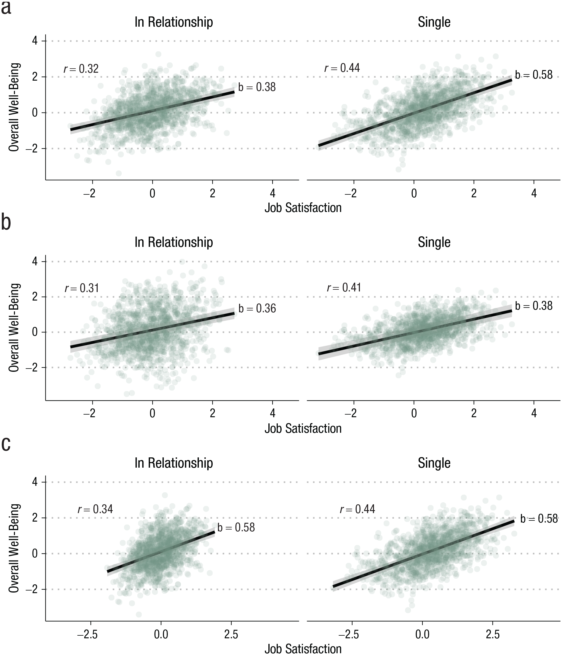
Relationship between job satisfaction and overall well-being for individuals in relationships and singles. (a) Scenario A: larger effect of job satisfaction among singles. (b) Scenario B: same effect, but there is less unexplained variability in well-being among singles. (c) Scenario C: same effect, but there is less variability in job satisfaction among singles. N = 50 people sampled on 50 days each. Data have been simulated

Another researcher thought about things in a different way. A one-point change in job satisfaction may have the same effect among both singles and individuals in a relationship. But being in a relationship is an additional source of variation in well-being that is independent of job satisfaction, and thus, partnered individuals will have more variance in their overall well-being that cannot be explained by job satisfaction. In this scenario, we have group differences in the residual variance $σ ²_{r e s i d u a l (y)}$ , which result in group differences in the standard deviation of the outcome $σ_{y}$ , and all else (slope, variance of the predictor) being equal, it would result in a higher correlation for singles than for partnered individuals but no differences in the moderation analysis (Fig. 3b).

As we mentioned above, another thing that could differ between groups is the variance in the predictor. For example, let us imagine that in our study, individuals who are in a relationship tend to have “settled down” with jobs that are overall more steady. Some of the singles, in contrast, have exciting jobs that come with more ups and downs. This corresponds to group differences in the variance of the predictor. If the slopes are the same in both groups, this will also lead to group differences in the variance of the outcome, but the differences in the variance of the predictor will be larger, and thus, the correlation will increase (Fig. 3c).

Choosing the appropriate model

Phrases that we routinely use to formulate verbal predictions, for example, “matters more,” “stronger influence,” or “more important for,” could refer both to steeper slopes or larger correlations. In psychology, in which many constructs are measured in abstract quantities like points on a Likert scale, standardized effect sizes (e.g., Pearson’s product-moment correlations or standardized regression coefficients) are so widespread that the distinction between slopes and correlations may often be lost. This focus on standardization has been criticized for more than 50 years (e.g., Tukey, 1969); for example, the epidemiologists Greenland et al. (1991) argued that the supposed comparability of standardized coefficients is purely illusory. As we have shown above, when it comes to interactions, the distinction between slopes and correlations matters a great deal because it affects whether we are actually testing our substantive hypotheses (e.g., Arnold, 1982, 1984).

As a first step, we need to be more specific about what our theory actually says (Hand, 1994). Verbal theory specification leaves room for ambiguities; formalizing our theories with the help of equations or computational models can remove these ambiguities (Smaldino, 2017) and force us to think more carefully about slopes and variances, along with many other assumptions and predictions. Going even further, the resulting statistical hypotheses could be reported in a machine-readable format that results in a maximum of clarity and transparency (Lakens & DeBruine, 2020). But even just a simple data simulation, such as the examples above, can help clarify the relationship between substantive hypothesis and patterns in the data. Once we have a better understanding of what we want to test, we can start thinking about the appropriate statistical model.

If a difference between slopes is of interest, we are firmly in the territory of interactions and may, for example, simply include the product term between the variables of interest. But what should we do if our hypothesis concerns the variance components? It may be tempting to simply compare correlations, but as we have shown above, correlations are sensitive to differences in slope, differences in the variance of the predictor, and differences in the variance of the outcome. Thus, depending on our hypothesis of interest, the correlation coefficient may be too “coarse” and miss important patterns in the data, and we should instead explicitly model the variance of interest.

Once again, the flexibility of brms pays off—it allows us to implement distributional models in a straightforward manner (Bürkner, 2020; Umlauf & Kneib, 2018). To understand how these models work, let us quickly think about what a simple “regular” regression model does. In a standard regression model, we are predicting an outcome that is normally distributed. This normal distribution is described by two parameters: its mean and its standard deviation (which captures the residual unexplained by our model). When we include predictors, these variables explain the first parameter, the mean of the normal distribution; the standard deviation is assumed to be constant across all observations. A distributional model additionally allows us to include predictors to explain the second parameter, the residual standard deviation.

We can use this approach to simply test, for example, whether a continuous variable has an effect on the standard deviation of another variable. If we additionally include predictors for the mean, we can then test whether the residual standard deviation—the variability not explained by the predictors included for the mean—varies depending on the level of some third variable. Concerning our example above, we could simultaneously test for an interaction in the narrower sense (difference in slopes) and for group differences in the residual standard deviation (differences in unexplained outcome variability) by running the following model in brms:

bf(overall_well_being ~ job_satisfaction * single, sigma ~ single)

The first line represents the standard interaction analysis that can be interpreted in the usual manner. The second line allows the residual standard deviation to vary depending on whether individuals are single. Here, a negative coefficient would indicate that the residual standard deviation is smaller among singles, which captures the idea that there is less unexplained variability among singles because they lack a romantic relationship that constitutes a major source of variability in well-being. On OSF, we provide more detailed code examples (osf.io/apxtv).

Substantive examples

Individual importance weighting

Rohrer and Schmukle (2018) investigated importance weighting—the idea that individuals judge the overall quality of their lives by aggregating their satisfaction with various life domains. In this model, more important domains receive higher weight, and in the literature, this is normally captured by including interactions between domain satisfaction and domain importance ratings (e.g., by including the product term, Importance Rating of Health × Satisfaction With Health). However, after publication, we discussed whether importance weighting could also be interpreted as improved prediction—for example, when regressing overall life satisfaction on health satisfaction, there should be less unexplained variance among individuals who consider health very important for their health. The substantive literature on the topic does not take a clear stance on what exactly is meant by weighting because it mostly relies on vague verbalizations, which probably go unchallenged because the underlying notion (“things that are important matter more”) is so intuitive.

Partner preferences after entering a relationship

Gerlach et al. (2019) investigated the stability of partner preferences in a sample of singles. At Time 2, a substantial proportion of participants had entered a new relationship. Gerlach et al. were interested in whether partner preferences changed more among participants who found a partner. In a standard moderation analysis, the slope of partner preferences at Time 1 on preferences at Time 2 was highly similar among singles and participants who found a partner. For example, on average, people who expressed a strong preference for attractiveness at Time 1 did so again at Time 2, regardless of whether they had found a partner in the meantime. However, among singles, the individual data points were closer to the regression line—at Time 2, they deviated less from their preference at Time 1—which resulted in a higher correlation across time. Individuals who had found a partner had adapted their preferences to better match the traits of their actual partners (e.g., if their partner fell short of their preference for attractiveness at Time 1, they reported a weaker preference for attractiveness at Time 2). This adaptation to the partner reduced the correlation with preferences at Time 1 but not the slope.

Meta-analysis of standardized effect sizes

Meta-analysts commonly investigate standardized effect sizes, such as correlation coefficients, across studies. These may conflate differences related to the research question (differences in slope, in the magnitude of effects) with unrelated differences (differences in variances, e.g., because of measurement error in the outcome variable, range restriction in the predictor). This leaves researchers at risk of spurious inferences about effect size heterogeneity, publication bias, and between-studies moderators (Wiernik & Dahlke, 2020). So should we instead aggregate unstandardized effects? Unfortunately, the lack of standardization in psychology means that effects are difficult to bring to a single metric by means other than standardization using the observed standard deviation and mean (but consider e.g., the percentage of the maximum possible; Cohen et al., 1999). Luckily, there are productive ways forward. Researchers can explicitly account for measurement error and selection effects (Wiernik & Dahlke, 2020). Furthermore, with well-validated instruments, such as IQ tests, standardization with norm data (rather than with data from the sample, which may vary in idiosyncratic ways) could avoid the problems discussed here. As a side effect, this would also allow researchers to quickly notice when a sample covers only a restricted range of values (e.g., because only psychology students were included).

Causal Identification of Interactions

Correlation does not imply causation—that much is clear. Researchers who rely on nonexperimental data need to make strong assumptions if they want to make causal claims (for an introduction, see e.g., Rohrer, 2018). But it may not be immediately clear what this implies for interactions. For example, what happens if we run an experiment but want to see how the manipulation interacts with some other variable that has not been manipulated? This is the scenario we are going to consider in the following. If none of the supposedly interacting variables have been manipulated (i.e., the data are observational), the concerns we discuss apply to both of them, and causal identification becomes even harder.

Motivating example

A group of researchers is interested in how a stress-reduction program affects participants’ subsequent subjective well-being. For this purpose, participants are randomly assigned to either participate in the treatment or in a control condition. Furthermore, the researchers are interested in how the intervention interacts with participants’ personality, which they assessed before the intervention took place.

In their first analysis, they regress subjective well-being at the end of the study on (a) a binary indicator of whether participants were in the treatment condition; (b) participants’ neuroticism, measured before the intervention took place; and (c) the product of the two variables. Table 3, Analysis 1 shows the results from this analysis.

Table 3.

Results From a Regression Analysis Predicting Subjective Well-Being From Treatment, Neuroticism, and Their Interaction, Plus Gender (Analysis 2), Plus the Interaction Between Treatment and Gender (Analysis 3)

Variable	Analysis 1		Analysis 2		Analysis 3
Variable	b	95% CI	b	95% CI	b	95% CI
Treatment yes/no	2.85	[2.68, 3.01]	2.88	[2.73, 3.03]	2.11	[1.92, 2.29]
Neuroticism	0.06	[−0.04, 0.15]	−0.09	[−0.18, −0.01]	0.05	[−0.04, 0.13]
Treatment × Neuroticism	0.38	[0.25, 0.51]	0.33	[0.21, 0.45]	−0.02	[−0.16, 0.11]
Female gender	—	—	0.92	[0.77, 1.07]	0.06	[−0.14, 0.24]
Treatment × Female Gender	—	—	—	—	1.84	[1.57, 2.13]

Note: N = 1,000. Data have been simulated. CI = credible interval.

These numbers suggest that the treatment interacts with the neuroticism of the treated individual, with bigger treatment effects among the more neurotic. However, the researchers are aware that women have reliably higher neuroticism than men, and one of them suggests that female gender should thus be statistically controlled for. The results from their second analysis can be found in Table 3, Analysis 2. The statistical evidence for the interaction remains mostly unaffected. Thus, they provisionally conclude that even controlling for female gender, the treatment still has bigger effects among the more neurotic.

But then a colleague makes them aware of a blog post that highlights that interactions require “interaction controls” (Simonsohn, 2019; see also Yzerbyt et al., 2004), and so they dutifully run a third analysis. Lo and behold, their third analysis reveals an interaction between female gender and treatment, but the interaction with neuroticism that was initially of interest has disappeared (Table 3, Analysis 3).⁴

The question of causality

The previous example demonstrates that the statistically significant coefficient of the interaction term does not imply a causal interaction. A causal interaction refers to a scenario in which (hypothetically) intervening on the third variable would change the effect of the treatment (for formalized definitions, see VanderWeele, 2009). This may often be the intended meaning when psychologists hypothesize interactions. In the example above, the researchers may have speculated that there is something about the treatment that makes it more effective for neurotic individuals not because of their gender but because of their neuroticism—it may target particular cognitive processes such as anxiety and worries that affect them more frequently.

Experiments are the ideal design to identify and test causal interactions. If both the treatment and the third variable have been manipulated by the researcher, a causal interpretation is warranted. Factorial experiments, which are frequently evaluated with the help of ANOVAs, neatly illustrate the symmetric nature of causal interactions. If two variables A and B interact causally, it is appropriate to state that the effect of A depends on the level of B, just as it is appropriate to state that the effect of B depends on the level of A.

Of course, experimental investigations are not always feasible or even just possible, and so researchers might sometimes want to consider an interaction in which one or both of the variables were not randomized. In such a scenario, inferring a causal interaction is equal to inferring causation from correlation—an endeavor that heavily depends on domain expertise and additional assumptions (for an introduction, see e.g., Rohrer, 2018). One step into this direction, as illustrated in the example above, consists of the control of third variables that confound the association between the nonrandomized variable and the outcome. However, establishing a causal interaction through third-variable control requires strong assumptions about the causal graph, such as the absence of unobserved confounding. Furthermore, interactive control is necessary, and in practice, the inclusion of multiple interactions at once can lead to unstable estimates. Variable selection procedures can reduce variance and thus aid estimation (Blackwell & Olson, 2020), but as always, this needs to be balanced against potential bias (for more on this general trade-off, see Yarkoni & Westfall, 2017).

What if a causal interaction cannot be established? It may still be of interest that the magnitude of the causal effect of one variable correlates with a third variable. Different terminology has been employed to describe such a situation. VanderWeele (2009) used the term effect modification (in contrast to interaction), Hernán and Robins (2010) talked about surrogate effect modifiers (in contrast to causal effect modifiers), and some psychologists talk about statistical interaction (in contrast to moderation or causal interaction). For example, in a clinical trial, it might be of interest to see how effective the treatment is within different subpopulations. Researchers might find out that the treatment works best among individuals with certain comorbidities, and that information might be helpful for treatment planning regardless of whether it is the other condition or one of its causes that causally affects the treatment effect. Although causal interactions are symmetric, the mere correlation between a third variable and the effect of another variable can be asymmetric. In our example above, neuroticism correlates with the effect of the treatment, but the treatment does not correlate with the effect of neuroticism—in fact, the data have been simulated so that neuroticism has no causal effect on subjective well-being at all.

Substantive examples

Personality moderates the effects of mindfulness on well-being

Much in line with our simulated example, de Vibe et al. (2015) investigated whether personality (neuroticism and conscientiousness) moderates the effects of mindfulness training among students. They found that the intervention reduced mental distress particularly well among students with higher scores on neuroticism. Although their analysis contained control variables (gender and baseline values of the outcome), they did not include the interaction between those control variables and treatment and thus failed to account for alternative explanations (e.g., treatment effect may vary depending on gender, treatment effect may vary depending on initial level of mental distress). Thus, the data do not allow us to conclude a causal interaction. Nonetheless, the article prominently discussed interpretations of a causal interaction between neuroticism and treatment, such as differences in emotional reactivity.

Personality moderates the effects of cultural tightness on cultural adaptation

Geeraert et al. (2019) investigated how students participating in intercultural programs adapted culturally to their host countries. They found that adaptation was lower for host countries with tighter cultures (i.e., cultures in which norms are more rigidly imposed). But this effect was moderated by personality; for example, students scoring high on honesty-humility showed high cultural adaptation even in tight cultures. Their longitudinal analyses do not account for potential confounders between personality and cultural adaptation, and thus, no causal interaction can be concluded. Nonetheless, the discussion section invoked the fit between personality and social norms as an explanation, which clearly assumes a causal role of personality (i.e., if we could intervene on personality, we would expect that this has subsequent effects on adaptation to tight cultures). Note that the authors also suggested that poor fit between students and host countries may be very costly and that selection with an eye for personality fit might hence be sensible. This suggestion is justified regardless of whether a causal interaction occurs. If personality correlates with students’ ability to adapt to certain cultures, it can be used to make placement decisions.

Country-level gender equality moderates the effects of the Gender × Age interaction on self-esteem

Bleidorn et al. (2016) investigated cross-sectional age trajectories of self-esteem in a sample spanning 48 nations. Overall, they found that on average, men reported higher levels of self-esteem (i.e., a gender gap), and so did older individuals, with no significant interaction between age and gender on average. However, these associations significantly varied across countries. Thus, in exploratory analyses, the authors investigated whether country-level characteristics moderated gender-specific age trajectories (i.e., they investigated the triple-interaction term, Gender × Age × Country Characteristic). They found that in countries with higher gender equality, the gender gap in self-esteem shrank with age. Although it may be tempting to give a substantive causal interpretation to this pattern—women who, through increased gender equality, have better access to high-status jobs and the political sphere end up with higher self-esteem—the authors pointed out that gender equality is highly correlated with other country characteristics, such as GDP per capita and the Human Development Index. Thus, no causal interaction should be concluded; the actual cause of gender differences in age trajectories of self-esteem may lie in other factors.

Recommendations

A variable may correlate with the effect of another variable without a causal interaction between the two, and it is even possible that there is a causal interaction between two variables but one of them does not correlate with the effect of the other one (the equivalent of causation without correlation, although this requires that different effects cancel each other out; see VanderWeele, 2009). Thus, for researchers to arrive at the right conclusion, it is important that they can distinguish between the two scenarios—and determine which one is relevant in a given situation.

If the purpose is to test a specific hypothesis derived from a theory, a helpful question to consider is “Would I expect that an intervention on the third variable changes the effect of the other variable?” In the case of our example, “Would an intervention that reduces neuroticism, such as psychotherapy, reduce the treatment effect of our stress reduction intervention?” If the answer is yes, a causal interaction is of interest, and if the third variable cannot be manipulated, all the concerns of causal inference based on observational data apply (see e.g., Rohrer, 2018).

Of course, not all interaction questions arise a priori, and sometimes a researcher might be confronted with the coefficient of a product term and struggle to find the right interpretation. Here, helpful questions to consider could be, “Assuming that the main effect of the third variable was of central interest, would the present study design allow me to interpret it as a causal effect under reasonable assumptions?” If the answer is yes, one may conclude a causal interaction, conditional on said assumptions. These assumptions (e.g., no unobserved confounders) should be spelled out explicitly, and authors should be prepared to defend them. If the answer is no, subsequent interpretations should take into account that one cannot conclude that a manipulation of the third variable would change the effect of interest. Thus, the study may be uninformative with respect to the mechanism underlying differences in treatment effects.

Conclusion: Better Answers, Better Questions

In this article, we discussed three issues. First, conclusions about interactions depend on scaling decisions, and flawed measures can lead to spurious interactions. Second, moderation of slopes is not the same as moderation of correlations. Third, a statistically significant interaction term is not the same as causal interaction. If researchers are not aware of these distinctions, they might accidentally analyze the data in a manner that returns the technically correct answer to the wrong question (Hand, 1994). This disconnect between research questions and statistical analyses can result in misled conclusions.

These issues may seem daunting, and after considering how these issues interact (see Box 3), one may be tempted to conclude that the best course of action is to stop investigating interactions altogether. Some weaker variation of this notion may be defensible. Many psychologists seem enthusiastic about increasingly complex claims about interactions (“boundary conditions”), mediation (“processes,” “mechanisms”), and any combination of the two (Rohrer et al., 2021). This enthusiasm should be tempered: Complex claims require very large samples and strong designs, they come with methodological complications like the ones outlined above, and they require reliable knowledge about more basic aspects (e.g., measurement properties, response biases, main effects). Our enthusiasm for complex claims may actively hinder the quest for such reliable knowledge: Researchers are disincentivized from conducting “less exciting,” “less novel” basic research, and thus it is quite possible that we end up building on sand (for a similar argument, see Scheel et al., 2020).

Box 3.

Interaction Issues Interact

The three issues we consider here cannot be considered in isolation. When the issues interact and models become more complex, formal models, data simulation, and visualization are even more helpful. To give an example of how these issues interact, if we want to correctly estimate effects on residual variance, we cannot ignore that our measure has a ceiling and a floor. If we did, we would underestimate the residual variance whenever a value is at the scale’s lower or upper limit because values can deviate in only one direction. This could result in an illusory effect on residual variance if, for instance, the investigated moderator has a strong main effect, driving values to the limit. New statistical software, such as brms, makes it easy to formulate the appropriate distributional models (Bürkner, 2020) with small changes (e.g., it takes only a small tweak to switch from predicting the residual standard deviation in a Gaussian regression to predicting the discrimination parameter in an ordinal regression, which inversely relates to the standard deviation of the latent variable).

To give another example, if we would adjust our interaction effect for a potential confounder to better fit our causal model, we should also adjust for the confounder when estimating effects of the moderator on residual variance. Again, it is easy to estimate multiple effects on the residual standard deviation in brms but difficult to do the same in the more established framework of correlational analysis.

In the introduction, we wrote that questions of nonlinearity of interactions can be resolved by careful examination of the data, whereas the issues we discuss here often require us to interrogate our assumptions. However, if we observe only subsets of the data, for example, if we have an old and a young cohort in our study that were recruited in different ways, we could run into the question of causal identification. If we observe that age effects on our outcome of interest are flattened in the older group, is it because recruitment methods act as a moderator? Or is the effect of age simply nonlinear, but the two parts of the curve we can see look straight?

Finally, questions of scale dependence and linearity of effects also come up when predicting distributional parameters other than the mean, such as the residual standard deviation. Again, brms allows for distributional assumptions and link functions to be changed and for nonlinear effects on all distributional parameters to be estimated using, for instance, thin-plate splines (Bürkner, 2020).

At the same time, as we have shown throughout this article, the issues we discussed are not unique to interactions. Scale dependence has particular implications for interactions (which may disappear or even reverse), but researchers investigating main effects still need to consider which outcome scale they are interested in. Moderation of correlation does not imply moderation of slopes and vice versa, but more generally, correlations are not the same as regression coefficients, and psychologists may sometimes reflexively choose standardized metrics when they are not suitable. Interactions may be causal or not, but the same applies to all effect estimates from observational studies and sometimes even to effect estimates from experiments (e.g., Montgomery et al., 2018). Thus, researchers cannot avoid these conceptual challenges by avoiding claims about interactions.

Furthermore, we concur with Lakens and Caldwell (2019) that there are benefits of examining interactions. For example, they can involve predictions that are more specific than those involving only main effects, allowing for particularly informative tests of competing theories, and they may help address issues of generalizability across different populations. Thus, instead of putting interaction research on hiatus, we should strive for improved interaction research.

Approaching the issue from the empirical side, researchers should pay closer attention to the details of their data and their model. Classical regression diagnostics (Belsley et al., 1980), such as plotting fitted values against residuals, are often taught, occasionally practiced, and rarely reported. Such diagnostics can uncover where the model falls short, such as assuming homoskedasticity or ignoring ceiling and floor effects. In a Bayesian workflow, these diagnostics can be seen as special cases of posterior predictive checks (generating data from the model and comparing it with the real data, see Fig. 5; Gabry & Mahr, 2018; Gelman et al., 2020). Research articles frequently report estimates from linear models only and select simple slopes graphs, but this leaves readers in the dark about the details of the data. Following the recommendations by McCabe et al. (2018), raw data and estimates should instead be depicted in so-called small multiples with individual plots for several simple slopes. Online supplements also make it possible to habitually share diagnostic plots, especially for complex models in which simply graphing the raw data is insufficient to evaluate the model.

Fig. 5.

Posterior predictive checks for a simple interaction model based on three different data-generating processes. The distribution of the outcome is shown, along with model-predicted distributions for 10 samples. (a) The model distribution shows a good fit to the real data. (b) A floor effect is apparent in the real data but not part of the model. (c) Heteroskedasticity makes for an awkward fit between real data and model predictions.

As a pedagogical tool, we generated Figure 6, a triple triptych in homage to Anscombe’s quartet (Anscombe, 1973). Every row represents a different interaction scenario resulting in identical simple slopes plots (black lines) and linear regression results. The first row shows the “ideal” scenario, which many researchers will naively assume: Only the slopes differ by moderator level. The middle row shows how a floor effect in the measurement scale can cause the illusion of an interaction even though only main effects were simulated at the latent level. The third row shows a scenario in which slopes and correlations exhibit reverse patterns: While the slope increases with higher moderator values, the correlation decreases (i.e., in the low moderator panel, the values scatter the least from the regression line). Note that a researcher who runs only a linear model and reports the resulting coefficients and simple slopes would not be able to distinguish between these scenarios although they lead to different substantive conclusions.

Fig. 6.

A triptych in homage to Anscombe. Columns show levels of the moderator variable (M). X and M are the same across rows, whereas Y has been generated according to different scenarios but maintains the same mean and variance. The slopes estimated according to a simple linear interaction model (black lines) are the same across rows, but graphing the raw data shows that the data-generating processes were quite different. Shaded regions around the regression lines show 95% credible intervals.

Careful consideration of the details of the data is important, but as we noted in the beginning, it is not sufficient to solve the issues highlighted in this article. No amount of graphing can answer questions about scaling assumptions or causality or tell us what exactly our research question is and how it could be tested. This leads us to a broader underlying issue.

In an idealized scenario, one may start with a substantive research question and then choose the appropriate statistical analysis. One may mistakenly pick the wrong analysis, but course corrections are possible because the goal of the analysis is clear. If the research question was formulated as a generative model, finding flaws in the analysis strategy is even possible before data collection. In our experience, the actual research process often works quite differently. The research question is rather vague to begin with (“How do X and Y affect Z?”), and statistical analyses are chosen for a variety of reasons (e.g., domain norms, familiarity, publishability, implementation in popular statistical packages) but not for their capability of providing appropriate answers.

So the necessary course corrections may be much broader because the underlying problem concerns our research questions and theories (Hand, 1994; Muthukrishna & Henrich, 2019). Psychological theories are often vague verbalizations that accommodate many different readings and corresponding statistical models. Researchers might “theorize” that one construct interacts with another one but leave open what pattern is to be expected. Arguments about the empirical support for such a vague hypothesis are futile because it is not even established what exactly is being predicted. Thus, ultimately, some broader rethinking of the field may be necessary, with a stronger focus on formal modeling (Guest & Martin, 2020; McElreath, 2020; Smaldino, 2017), more rigorous theorizing, and more precise research questions.

Footnotes

Acknowledgements

We thank Felix Elwert for his valuable input provided over the course of multiple discussion, as well as Paul-Christian Bürkner, Daniël Lakens, and Stefan C. Schmukle for their helpful comments on an earlier version of this article. We thank Johannes Zimmermann, Eric Turkheimer, Wendy Johnson, and Drew H. Bailey for their feedback on the preprint, which led to additional changes.

Transparency

Action Editor: Alexa Tullett

Editor: Daniel J. Simons

Author Contributions

J. M. Rohrer and R. C. Arslan contributed equally. J. M. Rohrer and R. C. Arslan jointly generated the idea for the manuscript and wrote all sections in collaboration. Both of the authors approved the final manuscript for sub-mission.

ORCID iDs

Julia M. Rohrer

Ruben C. Arslan

Prior Versions

A preprint of the submitted manuscript is available at .

Notes

References

Norton

E. C.

(2003). Interaction terms in logit and probit models. Economics Letters, 80(1), 123–129. https://doi.org/10.1016/S0165-1765(03)00032-6

Anscombe

F. J.

(1973). Graphs in statistical analysis. The American Statistician, 27(1), 17–21. https://doi.org/10.1080/00031305.1973.10478966

Arnold

H. J.

(1982). Moderator variables: A clarification of conceptual, analytic, and psychometric issues. Organizational Behavior and Human Performance, 29(2), 143–174. https://doi.org/10.1016/0030-5073(82)90254-9

Arnold

H. J.

(1984). Testing moderator variable hypotheses: A reply to Stone and Hollenbeck. Organizational Behavior and Human Performance, 34(2), 214–224. https://doi.org/10.1016/0030-5073(84)90004-7

Beck

E. D.

Jackson

J. J.

(2020). A mega-analysis of personality prediction: Robustness and boundary conditions. PsyArXiv. https://doi.org/10.31234/osf.io/vsm9y

Belsley

D. A.

Kuh

Welsch

R. E.

(1980). Regression diagnostics: Identifying influential data and sources of collinearity. Wiley.

Blackwell

Olson

(2020). Reducing model misspecification and bias in the estimation of interactions [Working paper]. https://mattblackwell.org/files/papers/lasso-inters.pdf

Bleidorn

Arslan

R. C.

Denissen

J. J. A.

Rentfrow

P. J.

Gebauer

J. E.

Potter

Gosling

S. D.

(2016). Age and gender differences in self-esteem—A cross-cultural window. Journal of Personality and Social Psychology, 111(3), 396–410. https://doi.org/10.1037/pspp0000078

Bond

T. N.

Lang

(2019). The sad truth about happiness scales. The Journal of Political Economy, 127(4), 1629–1640. https://doi.org/10.1086/701679

10.

Bürkner

P.-C.

(2017). brms: An R package for Bayesian multilevel models using Stan. Journal of Statistical Software, 80(1), 1–28. https://doi.org/10.18637/jss.v080.i01

11.

Bürkner

P.-C.

(2018). Advanced Bayesian multilevel modeling with the R package brms. The R Journal, 10(1), 395–411. https://doi.org/10.32614/RJ-2018-017

12.

Bürkner

P.-C.

(2020). Estimating distributional models with brms. CRAN. https://cran.r-project.org/web/packages/brms/vignettes/brms_distreg.html

13.

Bürkner

P.-C.

Vuorre

(2019). Ordinal regression models in psychology: A tutorial. Advances in Methods and Practices in Psychological Science, 2(1), 77–101. https://doi.org/10.1177/2515245918823199

14.

Cohen

Aiken

L. S.

West

S. G.

(1999). The problem of units and the circumstance for POMP. Multivariate Behavioral Research, 34(3), 315–346. https://doi.org/10.1207/S15327906MBR3403_2

15.

de Vibe

Solhaug

Tyssen

Friborg

Rosenvinge

J. H.

Sørlie

Halland

Bjørndal

(2015). Does personality moderate the effects of mindfulness training for medical and psychology students? Mindfulness, 6(2), 281–289. https://doi.org/10.1007/s12671-013-0258-y

16.

Gabry

Mahr

(2018). bayesplot: Plotting for Bayesian models. CRAN. https://CRAN.R-project.org/package=bayesplot

17.

Geeraert

Ward

Gelfand

Demes

K. A.

(2019). A tight spot: How personality moderates the impact of social norms on sojourner adaptation. Psychological Science, 30(3), 333–342. https://doi.org/10.1177/0956797618815488

18.

Gelman

(2018). You need 16 times the sample size to estimate an interaction than to estimate a main effect. https://statmodeling.stat.columbia.edu/2018/03/15/need-16-times-sample-size-estimate-interaction-estimate-main-effect/

19.

Gelman

Vehtari

Simpson

Margossian

C. C.

Carpenter

Yao

Kennedy

Gabry

Bürkner

P.-C.

Modrák

(2020). Bayesian workflow. arXiv. http://arxiv.org/abs/2011.01808

20.

Gerlach

T. M.

Arslan

R. C.

Schultze

Reinhard

S. K.

Penke

(2019). Predictive validity and adjustment of ideal partner preferences across the transition into romantic relationships. Journal of Personality and Social Psychology, 116(2), 313–330. https://doi.org/10.1037/pspp0000170

21.

Giner-Sorolla

(2018). Powering your interaction. Ap-proaching Significance. https://approachingblog.wordpress.com/2018/01/24/powering-your-interaction-2

22.

Greenland

Maclure

Schlesselman

J. J.

Poole

Morgenstern

(1991). Standardized regression coefficients: A further critique and review of some alternatives. Epidemiology, 2(5), 387–392.

23.

Guest

Martin

A. E.

(2020). How computational modeling can force theory building in psychological science. Perspectives on Psychological Science. Advance online publication. https://doi.org/10.1177/1745691620970585

24.

Hainmueller

Mummolo

(2019). How much should we trust estimates from multiplicative interaction models? Simple tools to improve empirical practice. Political Analysis, 27(2), 163–192. https://doi.org/10.1017/pan.2018.46

25.

Hand

D. J.

(1994). Deconstructing statistical questions. Journal of the Royal Statistical Society. Series A, 157(3), 317–356. https://doi.org/10.2307/2983526

26.

Hernán

M. A.

Robins

J. M.

(2010). Causal inference: What if. CRC Press.

27.

Huang

F. L.

(2019). Alternatives to logistic regression models in experimental studies. Journal of Experimental Education. Advance online publication. https://doi.org/10.1080/00220973.2019.1699769

28.

Johnson

(2007). Genetic and environmental influences on behavior: Capturing all the interplay. Psychological Review, 114(2), 423–440. https://doi.org/10.1037/0033-295X.114.2.423

29.

Lakens

(2020). Effect sizes and power for interactions in ANOVA designs. https://daniellakens.blogspot.com/2020/03/effect-sizes-and-power-for-interactions.html

30.

Lakens

Caldwell

A. R.

(2019). Simulation-based power-analysis for factorial ANOVA designs. PsyArXiv. https://doi.org/10.31234/osf.io/baxsf

31.

Lakens

DeBruine

L. M.

(2020). Improving transparency, falsifiability, and rigour by making hypothesis tests machine readable. Advances in Methods and Practices in Psychological Science. Advance online publication. https://doi.org/10.1177/2515245920970949

32.

Liddell

T. M.

Kruschke

J. K.

(2018). Analyzing ordinal data with metric models: What could possibly go wrong? Journal of Experimental Social Psychology, 79, 328–348. https://doi.org/10.1016/j.jesp.2018.08.009

33.

Loftus

G. R.

(1978). On interpretation of interactions. Memory & Cognition, 6(3), 312–319. https://doi.org/10.3758/BF03197461

34.

Mayer

Dietzfelbinger

Rosseel

Steyer

(2016). The EffectLiteR approach for analyzing average and conditional effects. Multivariate Behavioral Research, 51(2–3), 374–391. https://doi.org/10.1080/00273171.2016.1151334

35.

McCabe

C. J.

Halvorson

M. A.

King

Cao

Kim

(2020). Interpreting interaction effects in generalized linear models of nonlinear probabilities and counts. PsyArXiv. https://doi.org/10.31234/osf.io/th94c

36.

McCabe

C. J.

Kim

D. S.

King

K. M.

(2018). Improving present practices in the visual display of interactions. Advances in Methods and Practices in Psychological Science, 1(2), 147–165. https://doi.org/10.1177/2515245917746792

37.

McElreath

(2020). Statistical rethinking: A Bayesian course with examples in R and STAN. CRC Press.

38.

Montgomery

J. M.

Nyhan

Torres

(2018). How conditioning on posttreatment variables can ruin your experiment and what to do about it: Stop conditioning on posttreatment variables in experiments. American Journal of Political Science, 62(3), 760–775. https://doi.org/10.1111/ajps.12357

39.

Murray

A. L.

Molenaar

Johnson

Krueger

R. F.

(2016). Dependence of gene-by-environment interactions (GxE) on scaling: Comparing the use of sum scores, transformed sum scores and IRT scores for the phenotype in tests of GxE. Behavior Genetics, 46(4), 552–572. https://doi.org/10.1007/s10519-016-9783-5

40.

Mustillo

S. A.

Lizardo

O. A.

McVeigh

R. M.

(2018). Editors’ comment: A few guidelines for quantitative submissions. American Sociological Review, 83(6), 1281–1283. https://doi.org/10.1177/0003122418806282

41.

Muthukrishna

Henrich

(2019). A problem in theory. Nature Human Behaviour, 3(3), 221–229. https://doi.org/10.1038/s41562-018-0522-1

42.

Open Science Collaboration, Aarts

A. A.

Anderson

J. E.

Anderson

C. J.

Attridge

P. R.

Attwood

Axt

Babel

Bahník

Š.

Baranski

Barnett-Cowan

Bartmess

Beer

Bell

Bentley

Beyan

Binion

Borsboom

Bosch

. . . Zuni

(2015). Estimating the reproducibility of psychological science. Science, 349(6251), Article aac4716. https://doi.org/10.1126/science.aac4716

43.

Rohrer

J. M.

(2018). Thinking clearly about correlations and causation: Graphical causal models for observational data. Advances in Methods and Practices in Psychological Science, 1(1), 27–42. https://doi.org/10.1177/2515245917745629

44.

Rohrer

J. M.

Hünermund

Arslan

R. C.

Elson

(2021). That’s a lot to PROCESS! Pitfalls of popular path models. PsyArXiv. https://doi.org/10.31234/osf.io/paeb7

45.

Rohrer

J. M.

Schmukle

S. C.

(2018). Individual importance weighting of domain satisfaction ratings does not increase validity. Collabra Psychology, 4(1), Article 6. https://doi.org/10.1525/collabra.116

46.

Roser

Ritchie

Ortiz-Ospina

Hasell

(2020). Coronavirus pandemic (COVID-19). Our World in Data.

47.

Rothman

K. J.

Greenland

Walker

A. M.

(1980). Concepts of interaction. American Journal of Epidemiology, 112(4), 467–470. https://doi.org/10.1093/oxfordjournals.aje.a113015

48.

Scheel

A. M.

Tiokhin

Isager

P. M.

Lakens

(2020). Why hypothesis testers should spend less time testing hypotheses. Perspectives on Psychological Science. Advance online publication. https://doi.org/10.1177/1745691620966795

49.

Simonsohn

(2017). [57] Interactions in logit regressions: Why positive may mean negative. Datacolada. http://datacolada.org/57

50.

Simonsohn

(2019). [80] Interaction effects need interaction controls. Datacolada. http://datacolada.org/80

51.

Smaldino

P. E.

(2017). Models are stupid, and we need more of them. In Vallacher

R. R.

Read

S. J.

Nowak

(Eds.), Computational social psychology (pp. 311–331). Routledge.

52.

Smithson

(2012). A simple statistic for comparing moderation of slopes and correlations. Frontiers in Psychology, 3, Article 231. https://doi.org/10.3389/fpsyg.2012.00231

53.

Tukey

J. W.

(1969). Analyzing data: Sanctification or detective work? The American Psychologist, 24(2), 83–91. https://doi.org/10.1037/h0027108

54.

Umlauf

Kneib

(2018). A primer on Bayesian distributional regression. Statistical Modelling, 18(3–4), 219–247. https://doi.org/10.1177/1471082X18759140

55.

VanderWeele

T. J.

(2009). On the distinction between interaction and effect modification. Epidemiology, 20(6), 863–871. https://doi.org/10.1097/EDE.0b013e3181ba333c

56.

von Hippel

P. T.

Hamrock

(2019). Do test score gaps grow before, during, or between the school years? Measurement artifacts and what we can know in spite of them. Sociological Science, 6, 43–80.

57.

Wagenmakers

E.-J.

Krypotos

A.-M.

Criss

A. H.

Iverson

(2012). On the interpretation of removable interactions: A survey of the field 33 years after Loftus. Memory & Cognition, 40(2), 145–160. https://doi.org/10.3758/s13421-011-0158-0

58.

Westreich

Greenland

(2013). The table 2 fallacy: Presenting and interpreting confounder and modifier coefficients. American Journal of Epidemiology, 177(4), 292–298. https://doi.org/10.1093/aje/kws412

59.

Wiernik

B. M.

Dahlke

J. A.

(2020). Obtaining unbiased results in meta-analysis: The importance of correcting for statistical artifacts. Advances in Methods and Practices in Psychological Science, 3(1), 94–123. https://doi.org/10.1177/2515245919885611

60.

Yarkoni

Westfall

(2017). Choosing prediction over explanation in psychology: Lessons from machine learning. Perspectives on Psychological Science, 12(6), 1100–1122. https://doi.org/10.1177/1745691617693393

61.

Yzerbyt

V. Y.

Muller

Judd

C. M.

(2004). Adjusting researchers’ approach to adjustment: On the use of covariates when testing interactions. Journal of Experimental Social Psychology, 40(3), 424–431.

Supplementary Material

Please find the following supplemental material available below.

For Open Access articles published under a Creative Commons License, all supplemental material carries the same license as the article it is associated with.

For non-Open Access articles published, all supplemental material carries a non-exclusive license, and permission requests for re-use of supplemental material or any part of supplemental material shall be sent directly to the copyright owner as specified in the copyright notice associated with the article.

0.00 MB

Precise Answers to Vague Questions: Issues With Interactions

Abstract

Keywords

Now You See It, Now You Don’t: Interactions Are Scale Dependent

Motivating example

Which interpretation is the correct one?

The scale dependence of interactions, main effects, and everything

Floor and Ceiling Effects

Substantive examples

Flattening the curve

Summer break gaps

The paradox of declining female happiness

Recommendations

Same Slope Does Not Imply Same Correlation

Motivating example

Likewise, Same Correlation Does Not Imply Same Slope

Choosing the appropriate model

Substantive examples

Individual importance weighting

Partner preferences after entering a relationship

Meta-analysis of standardized effect sizes

Causal Identification of Interactions

Motivating example

The question of causality

Substantive examples

Personality moderates the effects of mindfulness on well-being

Personality moderates the effects of cultural tightness on cultural adaptation

Country-level gender equality moderates the effects of the Gender × Age interaction on self-esteem

Recommendations

Conclusion: Better Answers, Better Questions

Interaction Issues Interact

Footnotes

Acknowledgements

Transparency

ORCID iDs

Prior Versions

Notes

References

Supplementary Material