Sage Journals: Discover world-class research

Abstract

Measurement quality has recently been highlighted as an important concern for advancing a cumulative psychological science. An implication is that researchers should move beyond mechanistically reporting coefficient alpha toward more carefully assessing the internal structure and reliability of multi-item scales. Yet a researcher may be discouraged upon discovering that a prominent alternative to alpha, namely, coefficient omega, can be calculated in a variety of ways. In this Tutorial, I alleviate this potential confusion by describing alternative forms of omega and providing guidelines for choosing an appropriate omega estimate pertaining to the measurement of a target construct represented with a confirmatory factor analysis model. Several applied examples demonstrate how to compute different forms of omega in R.

Keywords

alpha psychometrics reliability R confirmatory factor analysis assessment omega measurement open data open materials

Measurement is an important aspect of the replication crisis facing psychology and related fields (Fried & Flake, 2018; Loken & Gelman, 2017), and it is well known that measurement error produces biased estimates of the associations among constructs that observed variables represent (e.g., Cole & Preacher, 2014). Yet researchers often present very little reliability and validity evidence for their variables, frequently reporting only coefficient alpha to convey the psychometric quality of tests (Flake, Pek, & Hehman, 2017). Furthermore, psychometricians have established that alpha is based on a highly restricted (and thus unrealistic) psychometric model and consequently can provide misleading reliability estimates (e.g., Sijtsma, 2009). The persistent popularity of alpha suggests that applied researchers are not aware of its limitations or alternative reliability estimates.

Although many reliability estimates have been presented in the literature, distinguishing among them and their software implementations can be confusing. In this Tutorial, I describe the calculation of different forms of coefficient omega (McDonald, 1999), which are reliability estimates calculated from parameter estimates of factor-analytic models specified to represent associations between a test’s items and the test’s target construct. Thus, being informed of a test’s internal factor structure is inherent in choosing an appropriate omega estimate. The main purposes of this Tutorial are to clarify distinctions among different omega estimates and to demonstrate how they can be calculated using routines readily available in R (R Core Team, 2018). Throughout, I use example data to illustrate these reliability estimates.

Disclosures

The complete R code and output (as a single .rmd file and resulting .pdf file) for the examples presented, data files, and a supplementary document describing additional analyses are available on OSF, at https://osf.io/m94rp/.

What Is Reliability?

Observed scores on any given psychological test or scale are determined by a combination of systematic (signal) and random (noise) influences. Reliability is defined as a population-based quantification of measurement precision (e.g., Mellenbergh, 1996) as a function of the signal-to-noise ratio. Measurement error, or unreliability, produces biased estimates of effects meant to represent true associations among constructs (Bollen, 1989; Cole & Preacher, 2014), and measurement error is a culprit in the replication crisis (Loken & Gelman, 2017). Thus, using tests with maximally reliable scores and using statistical methods to account for measurement error (e.g., Savalei, 2019) can help psychology progress as a replicable science; calculating and reporting accurate reliability estimates is integral to this goal.

Although the reliability concept pertains to any empirical measurement, this Tutorial focuses on composite reliability, that is, the reliability of observed scores calculated as composites (i.e., the sum or mean) of individual test components. These individual components are most commonly items within a test or scale. A formal definition of composite reliability based on classical test theory (CTT; e.g., Lord & Novick, 1968) first posits that an observed score x for individual test taker i on item j equals the individual’s true score t for that item plus an error score e:

x_{i j} = t_{i j} + e_{i j} .

Next, if X_i denotes an individual’s observed total score, calculated by summing¹ the observed item scores (i.e., X_i = $\sum_{j = 1}^{J} x_{i j}$ ), and if T_i denotes the individual’s total true score, which is the sum of the unobserved true scores (T_i = $\sum_{j = 1}^{J} t_{i j}$ ), then the reliability ρ_X of total-score variable X is the proportion of total true-score variance relative to total observed variance:

ρ_{X} = \frac{σ_{T}^{2}}{σ_{X}^{2}} .

Because true scores are unobserved, reliability cannot be calculated directly from this formula, which has led to the development of various approaches to estimating reliability, most prominently coefficient alpha (Cronbach, 1951). (See Revelle & Condon, 2019, for a review relating composite reliability, test-retest reliability, and interrater reliability to this formal variance-ratio definition of reliability.)

It is important to recognize that the CTT true score does not necessarily equate to a construct score (Borsboom, 2005). Thus, a true score may be determined by a construct that a test is designed to measure (the target construct) as well as by other systematic influences. Most often, researchers want to know how reliably a test measures the target construct itself, and for this reason it is important to establish the dimensionality, or internal structure, of a test before estimating reliability (Savalei & Reise, 2019). Factor analysis is commonly used to investigate and confirm the internal structure of a multi-item test, and as shown throughout this Tutorial, parameter estimates of factor-analytic models lead to reliability estimates representing how precisely test scores measure target constructs represented by the models’ factors. In this framework, a one-factor model is adequate to explain the item-response data of a unidimensional test measuring a single target construct; conversely, poor fit of a one-factor model is evidence of multidimensionality. The formal definition of reliability from CTT can be adapted to this context so that reliability is the proportion of a scale score’s variance explained by a target construct (Savalei & Reise, 2019). Therefore, it is crucial to determine how a test represents that construct with respect to its internal factor structure. If reliability is estimated using the parameters of an incorrect (i.e., misspecified) factor model, then the reliability estimate is likely to be biased with respect to the measurement of the target construct. The key idea to this Tutorial is that a reliability coefficient should estimate how well an observed test score measures a target construct, which does not necessarily correspond to how well the score captures replicable variation because some replicable variation may be irrelevant to the target construct; thus, it is critical for the target construct to be accurately represented in a factor model for the test.

Because the reliability estimates presented herein are calculated from factor-analytic models, familiarity with factor analysis, especially confirmatory factor analysis (CFA; a type of structural equation modeling, or SEM), is beneficial. I emphasize the use of CFA over exploratory factor analysis (EFA) for reliability assessment because using CFA implies having strong, a priori hypotheses about the underlying causal associations between one or more target constructs (represented by the model’s factors) and observed item scores. In the preliminary stages of scale development, EFA is valuable for uncovering systematic influences on item responses that might map onto hypothesized constructs, whereas specification of a CFA model implies that the item-construct relations underpinning certain reliability estimates have been more well established (Flora & Flake, 2017; Zinbarg, Yovel, Revelle, & McDonald, 2006). Establishing these item-construct associations is critical for reliability to be meaningfully estimated because choice of an appropriate reliability estimate depends on the interpretation of the final measurement model chosen for a test (Savalei & Reise, 2019). For readers unfamiliar with CFA, I present basic principles that should enable use of the procedures presented here, but I strongly encourage such readers to acquire further background knowledge (e.g., see Brown, 2015).

This Tutorial focuses on forms of coefficient omega that estimate how reliably a total score for a test measures a single construct that is common to all items in the test, even if the test is multidimensional (e.g., a test designed to produce a total score as well as subscale scores). First, I demonstrate reliability estimation for unidimensional tests represented by one-factor models. Often, a test is designed to measure a single construct, but a one-factor model does not adequately represent the test’s internal structure. In this situation, reliability estimates based on a one-factor model are likely to be inaccurate, and instead reliability estimates should be based on a multidimensional (i.e., multifactor) model. In other situations, a test may be explicitly designed to measure multiple constructs (i.e., a test with subscales), but a meaningful total score is still of interest. Thus, after addressing the unidimensional case, I present omega estimates of total-score reliability for multidimensional tests; the online supplement addresses reliability assessment for subscale scores.

Reliability of Unidimensional Tests: Omega to Alpha

Figure 1 shows a path diagram of a one-factor model for a hypothetical 10-item test. Path diagrams represent latent variables, or factors, with ovals and represent observed variables (i.e., item-response variables in the present context) with rectangles. Linear associations are represented by straight, unidirectional arrows. For example, because the factor f and an error term e₁ are the two entities with arrows pointing at item x₁ in Figure 1, f and e₁ are the two linear influences on x₁. The arrow from f to x₁ is labeled as λ₁, which is a factor-loading parameter giving the strength of the association between f and x₁. The effects implied by these two arrows in the path diagram combine to form the linear regression equation

x_{1} = λ_{1} f + e_{1},

which indicates that item x₁ is a dependent variable regressed on the factor f as a single independent variable with slope coefficient λ₁ and error e₁. This one-factor model consists of an analogous equation for each observed item such that

x_{j} = λ_{j} f + e_{j},

where x_j is the jth item regressed on factor f with factor loading λ_j (the intercept term is omitted from this and other equations without loss of generality). This equation in which item scores are influenced by a single factor, but to varying degrees (i.e., λ_j varies across items), is known as the congeneric model in the psychometric literature. As shown later, when a model consists of more than one factor, this equation expands to a multiple regression equation with each x_j simultaneously regressed on multiple factors.

Fig. 1.

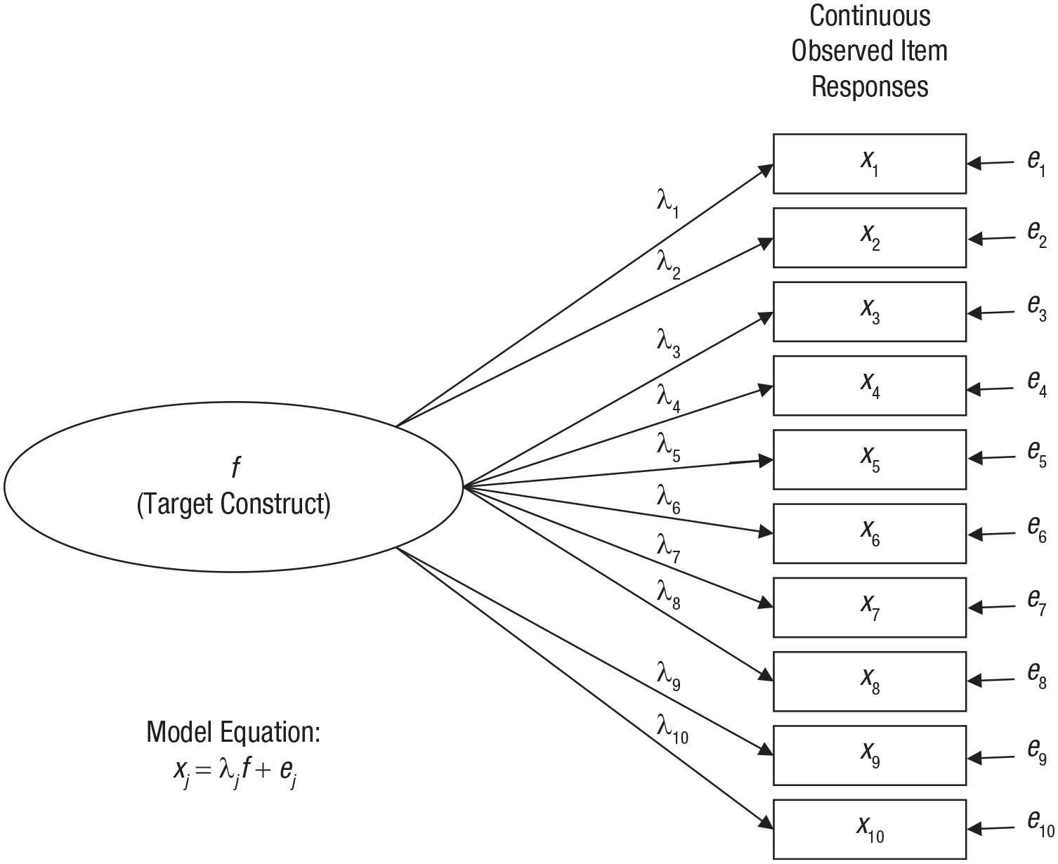
One-factor model for a unidimensional test consisting of 10 continuously scored items. See the text for further explanation.

Because scores on the factor f are unobserved, the λ_j factor-loading parameters cannot be estimated with the usual ordinary least squares method for linear regression. Instead, the factor loadings (and other model parameters) are estimated as a function of a covariance (or correlation) matrix among the observed item scores, typically using a maximum likelihood (ML) function. In addition to factor loadings, other model parameters include the factor variance and the variances of the individual error terms. Because the factor is unobserved, its scale is arbitrary, and the model cannot be estimated (i.e., the model is not identified) unless a parameter is constrained to define the factor’s scale. In all the examples in this Tutorial, I have set the scale of each factor by constraining its variance to be equal to 1 (which also serves to simplify equations for omega reliability estimates).² A variety of statistics is available to evaluate how well a CFA model fits the item-level data (and thereby evaluate the tenability of unidimensionality). In the examples presented, I report the root mean square error of approximation (RMSEA), comparative-fit index (CFI), and Tucker-Lewis index (TLI); smaller values (e.g., .08 or lower) of RMSEA are indicative of better model fit, whereas larger values (e.g., .90 or greater) of CFI and TLI indicate better model fit.

Coefficient omega

Numerous authors have shown that if the equation for the CTT true score is reexpressed as the one-factor model such that an individual’s true score t_ij for item j is presumed to equal the product of the item’s factor loading λ_j and the individual’s factor score f_i (i.e., t_ij = λ_jf_i ) and the factor variance is fixed to 1, then reliability is a function of the factor-loading parameters (e.g., Jöreskog, 1971; McDonald, 1999). Conceptually, because the factor loading quantifies the strength of the association between an item and a factor, the extent to which a set of items (as represented by their total score) reliably measures the factor is a function of the items’ factor loadings. Therefore, the reliability of the total score on a unidimensional test can be estimated from parameter estimates of a one-factor model fitted to the item scores. I refer to this reliability estimate as ω_u, and its formula is presented in Table 1: The numerator of ω_u represents the amount of total-score variance explained by the common factor f as a function of the estimated factor loadings (i.e., the numerator estimates the $σ_{T}^{2}$ term in the population reliability formula given earlier), and the denominator, ${\hat{σ}}_{X}^{2}$ , is the estimated variance of the observed total score. This formula gives a form of coefficient omega that is appropriate under the strong assumption that the one-factor model is correct, that is, the set of items is unidimensional, so that ω_u represents the proportion of total-score variance that is due to the single factor.³ The subscript u indicates that this variant of omega is based on a unidimensional model; different forms of coefficient omega introduced later are distinguished by different subscripts.

Table 1.

Formulas for Coefficient Omega Estimates for Three Underlying Factor Models

Model	Model equation(s)	Reliability estimate of total score X as a measure of a single construct common to all items
One-factor model (unidimensional, congeneric model), continuous items	x_j = λ_j f + e_j	$ω_{u} = \frac{{(\sum_{j = 1}^{J} {\hat{λ}}_{j})}^{2}}{{\hat{σ}}_{X}^{2}}$
One-factor model (unidimensional, congeneric model), categorical items	x_j = c if τ_jc < $x_{j}^{}$ ≤ τ_jc+1, $x_{j}^{}$ = λ_j f + e_j	$ω_{u - c a t} = \frac{\sum_{j = 1}^{J} \sum_{j' = 1}^{J} (\begin{array}{l} \sum_{c = 1}^{C - 1} \sum_{c' = 1}^{C - 1} Φ_{2} ({\hat{τ}}_{x_{j c}}, {\hat{τ}}_{x_{j' c'}}, {\hat{λ}}_{j} {\hat{λ}}_{j'}) - \\ (\sum_{c = 1}^{C - 1} Φ_{1} ({\hat{τ}}_{x_{j c}})) (\sum_{c' = 1}^{C - 1} Φ_{1} ({\hat{τ}}_{x_{j' c}})) \end{array})}{{\hat{σ}}_{X}^{2}}$
Bifactor model (hierarchical factor model), continuous items	$x_{j} = λ_{j g} g + (\sum_{k = 1}^{K} λ_{j k} s_{k}) + e_{j}$	$ω_{h} = \frac{{(\sum_{j = 1}^{J} {\hat{λ}}_{j g})}^{2}}{{\hat{σ}}_{X}^{2}}$

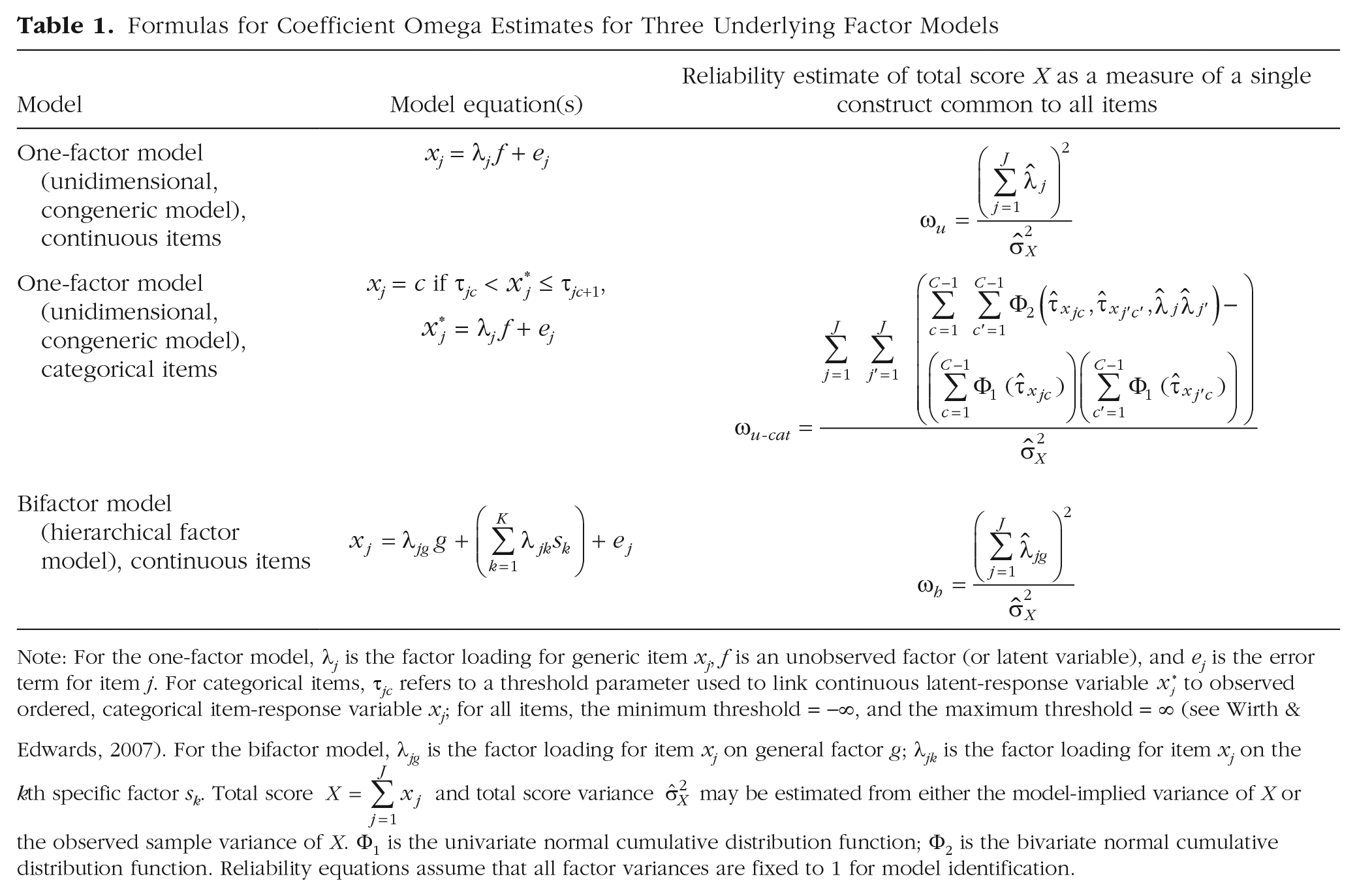
Note: For the one-factor model, λ_j is the factor loading for generic item x_j, f is an unobserved factor (or latent variable), and e_j is the error term for item j. For categorical items, τ_jc refers to a threshold parameter used to link continuous latent-response variable $x_{j}^{*}$ to observed ordered, categorical item-response variable x_j; for all items, the minimum threshold = −∞, and the maximum threshold = ∞ (see Wirth & Edwards, 2007). For the bifactor model, λ_jg is the factor loading for item x_j on general factor g; λ_jk is the factor loading for item x_j on the kth specific factor s_k. Total score $X = \sum_{j = 1}^{J} x_{j}$ and total score variance ${\hat{σ}}_{X}^{2}$ may be estimated from either the model-implied variance of X or the observed sample variance of X. Φ₁ is the univariate normal cumulative distribution function; Φ₂ is the bivariate normal cumulative distribution function. Reliability equations assume that all factor variances are fixed to 1 for model identification.

The ${\hat{σ}}_{X}^{2}$ term in the denominator of ω_u can be calculated either as the sample variance of the total score X or as the model-implied variance of X. Generally, this choice is unlikely to have a large effect on the magnitude of omega estimates if the estimated model is not badly misspecified (as evidenced by good model fit).⁴ Specifically, ${\hat{σ}}_{X}^{2}$ can be calculated as the sum of all elements in the variance-covariance matrix of item scores (which equals the sample variance of X) or as the sum of all elements in the model-implied covariance matrix among the observed items (i.e., the model-implied variance of X). Representing the total-score variance as a function of the entire model-implied covariance matrix incorporates any free covariances among the individual item-level error terms, e_j. Thus, when free error covariances are explicitly specified, the model-implied total-score variance used to calculate ω_u is a function of both error variances and the free error covariances. Although error covariances may represent replicable variation in observed test scores, these parameters are separate from variance due to the target construct represented by the common factor f, and thus error covariances contribute to the total observed variance (i.e., the denominator of ω_u) but not to variance due to the factor (i.e., the numerator of ω_u). The demonstration later in this discussion of ω_u shows how to obtain an ω_u estimate in R that accounts for the contribution of error covariances (when they are specified as free parameters rather than fixed to 0 by software defaults) to total variance by calculating the denominator of ω_u as a function of the entire model-implied covariance matrix among items.

After the one-factor model is estimated, one can obtain a residual covariance (or correlation) matrix to diagnose the presence of large error covariance between any pair of items; a residual covariance between two items is the difference between their observed covariance and the corresponding model-implied covariance. Green and Yang (2009a) described scenarios in which a unidimensional test might produce correlated errors, although large residual correlations may also be evidence of multidimensionality. Large residual correlations diminish the fit of the one-factor model to data, which can prompt researchers to modify their hypothesized CFA model to explicitly specify free error-covariance parameters.⁵

Coefficient alpha

If the population factor loadings are equal across all items, then the j subscript can be dropped from λ in the equation for the one-factor model, which leads to what is known as the essential tau-equivalence model. If this model is correct, it can be shown that ω_u is equivalent to alpha as long as the errors e_j remain uncorrelated (see McDonald, 1999, or Green & Yang, 2009a, for details). Taken together, alpha is an estimate of total-score reliability for the measurement of a single construct common to all items in a test under the conditions that (a) a one-factor model is correct (i.e., the test is unidimensional), (b) the factor loadings are equal across all items (i.e., essential tau equivalence), and (c) the errors e_j are independent across items. Because it is unlikely for all of these conditions to hold in any real situation, some researchers have called for abandoning alpha in favor of alternative reliability estimates (e.g., McNeish, 2018). However, Savalei and Reise (2019) contended that only severe violations of essential tau equivalence cause alpha to produce a notably biased reliability estimate, whereas multidimensionality and error correlation are more likely to be problematic for the interpretation of alpha as a reliability estimate for the measurement of a single target construct (Green & Yang, 2009a; Zinbarg et al., 2006), largely because alpha does not disentangle replicable variation due to a target construct from other sources of replicable variation.

Overall, estimates of ω_u are unbiased with varying factor loadings (i.e., violation of tau equivalence), when alpha underestimates population reliability (e.g., Zinbarg, Revelle, Yovel, & Li, 2005). Furthermore, Yang and Green (2010) showed that ω_u estimates are largely robust when the estimated model contains more factors than the true model, even with samples as small as 50. Trizano-Hermosilla and Alvarado (2016) found that increasing levels of skewness in the univariate item distributions produced increasingly negatively biased ω_u estimates, especially for short tests (i.e., six items in their study), but that item skewness caused greater bias for alpha than for ω_u.

Example calculation of ω_u in R

To demonstrate calculation of ω_u using R, I use data for five items measuring the personality trait openness as completed by 2,800 participants in the Synthetic Aperture Personality Assessment project (Revelle, Wilt, & Rosenthal, 2010). These data are available on this Tutorial’s OSF site as well as in the psych package for R (Revelle, 2020). These items have a 6-point, ordered categorical Likert-type response scale and thus are treated as continuous variables for CFA and reliability estimation; as I describe later, when items have fewer than five response categories, it is important to explicitly account for their categorical nature. With these data, alpha equals .60 for the five-item openness test, but one should not justify using alpha by merely assuming that the test is unidimensional and that its scores conform to the essential tau-equivalence model; rather, the test’s factor structure should be tested to determine an appropriate reliability estimate. Furthermore, it is important to note that I reverse-scored two negatively worded items (Items O2 and O5) before fitting one-factor CFA models to the data because not doing so would produce a mix of positive and negative factor loadings. Such a mix will reduce the numerator of ω_u and lead to a misleadingly low reliability estimate; the absolute strength of the factor loadings is what should matter in representing how well the items measure the factor.

For all examples in this Tutorial, I used the R package lavaan (Version 0.6-5; Rosseel, 2012) to estimate CFA models. Once a CFA model was estimated, functions from the semTools package (Version 0.5-3; Jorgensen, Pornprasertmanit, Schoemann, & Rosseel, 2020) were used to obtain reliability estimates based on the CFA model object created by lavaan. I have assumed that readers have some elementary familiarity with R, including how to install packages and manage data sets (files on the OSF site provide complete code corresponding to all examples in this Tutorial). The lavaan package is loaded as follows:

> library(lavaan)

In this example, I fitted the one-factor model depicted in Figure 1 to the data for the five openness items using direct ML estimation to incorporate cases with incomplete data (see Brown, 2015). The one-factor model (here named mod1f) is specified using a plain text string:

> mod1f <- ‘openness =~ O1 + O2 + O3 + O4 + O5’

This string indicates that a factor named openness is measured by the five observed variables listed on the right-hand side of the =~ operator; O1 through O5 are the names assigned to the openness items in the data frame (called open). Next, the model mod1f is estimated using the cfa function:

> fit1f <- cfa(mod1f, data=open, std.lv=T, missing=‘direct’, estimator=‘MLR’)

The std.lv option (referring to standardize latent variables) is set to TRUE so that the scale of the open factor is set by fixing its variance equal to 1, leaving all factor loadings as free parameters. The missing=‘direct’ option indicates that missing data are to be handled with direct ML estimation (see Brown, 2015), and the MLR estimator requests ML with robust model-fit statistics (see Savalei, 2018), as recommended by Rhemtulla, Brosseau-Liard, and Savalei (2012) to account for nonnormality inherent in the analysis of item-level data.

The results can be viewed using the summary function:

> summary(fit1f, fit.measures=T)

The fit.measures option is set to TRUE to request a set of commonly reported model-fit statistics, including the RMSEA, CFI, and TLI indices. The fit statistics reported under the Robust column in the summary indicate that this one-factor model has a marginal fit to the data; although the CFI of .94 suggests adequate fit, the TLI of .88 is lower than desired, and the RMSEA is somewhat high at 0.08; in combination, the indices cast doubt on the suitability of this one-factor model for subsequently obtaining a reliability estimate for the openness scale (see Brown, 2015, for discussion of assessing model fit using these and other statistics). Nonetheless, for illustrative reasons, I examine the factor-loading estimates and calculate ω_u before revising the CFA model to obtain a more appropriate ω_u estimate.

The factor-loading estimates of the fit1f model are listed under the Latent Variables heading in the results summary as follows:

Latent Variables:

Estimate Std.Err z-value P(>|z|)

openness =~

O1 0.622 0.029 21.536 0.000

O2 0.684 0.042 16.466 0.000

O3 0.794 0.032 24.572 0.000

O4 0.361 0.031 11.779 0.000

O5 0.685 0.036 19.069 0.000

These estimates of $\hat{λ}$ vary substantially (from .36 to.79), suggesting that tau equivalence is not tenable for this openness test and thus that ω_u is a more appropriate reliability estimate than alpha.⁶ The ω_u estimate can be obtained by executing the reliability function from the semTools package (i.e., semTools::reliability) on the fit1f one-factor model object:

> library(semTools)

> reliability(fit1f)

This call to reliability produces the following output:

openness

alpha 0.5999111

omega 0.6079033

omega2 0.6079033

omega3 0.6078732

avevar 0.2461983

The results listed in the omega and omega2 rows give the ω_u estimate in which the denominator equals the model-implied variance of the total score X, and the results listed in the omega3 row are based on a variation in which the denominator equals the observed, sample variance of X, as described earlier.⁷ The resulting ω_u of .61 represents the proportion of total-score variance that is due to the single factor, that is, how reliably a total score for these five items measures an openness common factor.

As is any statistic calculated with sample data, ω_u is a point estimate of a population parameter and is subject to sampling error; thus, its precision can be conveyed with a confidence interval (CI). Kelley and Pornprasertmanit (2016) reviewed different approaches to constructing CIs around omega estimates, ultimately recommending bootstrapping. The ci.reliability function from the MBESS package (Kelley, 2019; Version 4.6.0) can be used to obtain CIs for some forms of omega. For the current example, a percentile bootstrap 95% CI for ω_u is obtained with

> library(MBESS)

> ci.reliability(data=open, type="omega", interval.type="perc")

The output gives $est as .61, the point estimate of ω_u, along with a 95% CI from .58 ($ci.lower) to .63 ($ci.upper), which represents a range of plausible values for the population ω_u.

Although the factor-loading estimates varied across items, the difference between ω_u and alpha (.61 vs. .60) is quite small. But, as mentioned earlier, when a one-factor model includes error correlations among items, the difference between ω_u and alpha can be substantial. In this case, the fit1f model has a small but notable residual correlation (r = .10) between the O2 and O5 items,⁸ which is not surprising because these were the two reverse-coded items. Thus, it may be important to account for the corresponding error covariance in the calculation of ω_u. To include this term as a free parameter, the one-factor model can be respecified as a new model, called mod1fR, as follows:

> mod1fR <- ‘openness =~ O1 + O2 + O3 + O4 + O5

O2 ~~ O5’

The second line uses the ~~ operator to specify the free error-covariance parameter. When this revised model is fitted to the data (see the OSF project page for complete code and output), the overall model fit is considerably improved (RMSEA = .04, CFI = .99, TLI = .97), and the estimate of the standardized error covariance (i.e., error correlation) equals .19. Next, applying the reliability function to the fitted model obtains a ω_u estimate of .56, which is notably lower than the .61 obtained from the first one-factor model, in which all error covariances were assumed to equal zero.⁹ Therefore, this example demonstrates the potential importance of explicitly modeling interitem error covariances when fitting a factor model from which ω_u is to be estimated. Because the overall model fit was improved and the error covariance is conceptually meaningful (because reverse-scored items often share excess covariance), the revised ω_u of .56 is more trustworthy than the first ω_u as an estimate of the composite reliability of the openness scale with respect to the measurement of a single openness factor.

Factor Analysis of Ordered, Categorical Items

Most often, item responses are scored with an ordered, categorical scale (e.g., Likert-type items scored with discrete integers) or a binary response scale (e.g., 1 = yes, 0 = no). These scales produce categorical data for which the traditional, linear factor-analytic model is technically incorrect; thus, fitting CFA models to the observed Pearson product-moment covariance (or correlation) matrix among item scores can produce inaccurate results (see Flora, LaBrish, & Chalmers, 2012). Just as binary or ordinal logistic regression is recommended over linear multiple regression for a categorical outcome, a categorical-variable method is recommended for factor analysis of categorical item scores: One can fit a CFA model to polychoric correlations, rather than product-moment covariance or correlations, to account for items’ categorical nature (see Finney & DiStefano, 2013). A polychoric correlation measures the bivariate association between two binary or ordinally scaled variables, explicitly accounting for its nonlinear nature, and is thus appropriate for representing the associations among items eliciting ordered, categorical responses. As the number of item-response categories increases (e.g., to five or more response options), the item scores may behave more like continuous variables, and so CFA estimates obtained with product-moment covariances become closer to results obtained with polychoric correlations (Rhemtulla et al., 2012).

CFA models can be readily fitted to polychoric correlations with most SEM software, including the lavaan package in R. Doing so subtly revises the one-factor model given earlier to

x_{j}^{*} = λ_{j} f + e_{j},

such that now the factor loading λ_j represents the strength of the linear association between the factor f and a latent-response variable $x_{j}^{*}$ , rather than the observed item-response variable x_j. This latent-response variable is an unobserved, continuous variable representing a respondent’s judgment about item content that determines the observed value of an ordinal item response as a function of threshold parameters (for further explanation, see Wirth & Edwards, 2007). Thus, the factor influences the observed, categorical variables indirectly via the latent-response variables. Figure 2 gives a path diagram of this one-factor model: The latent-response variables (depicted with small ovals) are linearly regressed on the single factor (as shown with straight arrows), whereas the jagged arrows represent thresholds linking the latent-response variables to the observed item-response variables (again depicted with rectangles); each jagged arrow represents one or more threshold parameters.¹⁰

Fig. 2.

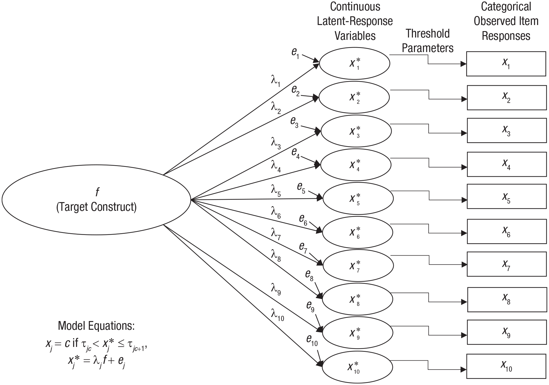
One-factor model for a unidimensional test consisting of 10 ordinally scaled items. See the text for further explanation.

Categorical omega

Because the factor loadings estimated from polychoric correlations represent the associations between the factor and latent-response variables rather than the observed item responses themselves, applying the ω_u formula presented earlier in this context would give the proportion of variance explained by the factor relative to the variance of the sum of the latent-response variables (i.e., $X^{*}$ = $\sum_{j = 1}^{J} x_{j}^{*}$ ) instead of the total variance of the sum of the observed item responses (i.e., X = $\sum_{j = 1}^{J} x_{j}$ ); that is, ω_u would represent the reliability of a hypothetical, latent total score instead of the reliability of the actual observed total score. To remedy this issue, Green and Yang (2009b) developed an alternative reliability estimate that is rescaled into the observed total-score metric. This reliability estimate for unidimensional categorical items is referred to as ω_u-cat; its formula is in Table 1. Although this formula is complex, its numerator, like that of ω_u, expresses the amount of observed total-score variance explained by the single factor. This term is obtained from applying the univariate and bivariate normal cumulative distribution functions (denoted as Φ₁ and Φ₂, respectively) based on the factor loadings and thresholds obtained when a CFA model is estimated using polychoric correlations; in short, the Φ₁ and Φ₂ functions transform the explained variance in the latent-response-variable metric back into the observed total-score metric. As for ω_u, the denominator of ω_u-cat is the estimated variance of the observed total score (i.e., ${\hat{σ}}_{X}^{2}$ ), which may be calculated as the sample variance of X or the model-implied variance of X according to the formula given in Green and Yang.

Yang and Green (2015) asserted that applied researchers should be more interested in the reliability of an observed total score X than in the reliability of a latent total score X^* because observed scores, rather than latent scores, are most frequently used to differentiate among individuals in research and practice. Yang and Green established that, compared with ω_u, ω_u-cat produces more accurate reliability estimates for total score X with ordinal item-level data, especially when the univariate item-response distributions differ across items.

Example calculation of ω_u-cat in R

To demonstrate estimation of ω_u-cat in R, I use data from a subsample of 500 participants who completed the four-item psychoticism scale by Jonason and Webster (2010) online via an open-access personality-testing website (https://openpsychometrics.org/about). With these data, alpha for the psychoticism scale was .77, but it should not be assumed that the scale is unidimensional and conforms to the essential tau-equivalence model; instead, its factor structure should be tested to determine an appropriate reliability estimate. Because the psychoticism items have a 4-point response scale, I fitted the one-factor model to the interitem polychoric correlations using WLSMV, a robust weighted least squares estimator that is recommended over the ML estimator for CFA with polychoric correlations (Finney & DiStefano, 2013).

Specifically, the one-factor model is specified in the same way as in the previous example with items treated as continuous variables:

> mod1f <- ‘psyctcsm =~ DDP1 + DDP2 + DDP3 + DDP4’

This code indicates that the factor psyctcsm is measured by observed variables DDP1 through DDP4, which are the names of the psychoticism items in the data frame. This mod1f model is also estimated using the cfa function:

> fit1f <- cfa(mod1f, data=potic, std.lv=T, ordered=T, estimator=‘WLSMV’)

But now, the ordered option is set to TRUE so that all items are treated as ordered, categorical variables; consequently, lavaan is told to fit the model to polychoric correlations using WLSMV. As before, the std.lv option is set to TRUE so that the variance of the psyctcsm factor is fixed equal to 1.

Again, the results can be viewed using the summary function. The model-fit statistics under the Robust column indicate that this one-factor model fits the data adequately, CFI = .99, TLI = .97; although the RMSEA has a high value of .11, the residual correlations are all small (< .07). Thus, it seems reasonable to estimate reliability of the psychoticism scale from the parameter estimates of this model (i.e., the scale can be considered a unidimensional test). As for ω_u, the ω_u-cat estimate can be obtained by executing the semTools::reliability function on the fit1f one-factor model object; because this model was fitted to polychoric correlations, semTools::reliability automatically calculates ω_u-cat instead of ω_u:

> reliability(fit1f)

This call to reliability produces the following output:

psyctcsm

alpha 0.8007496

omega 0.7902953

omega2 0.7902953

omega3 0.7932682

avevar 0.5289638

Results listed in the omega and omega2 rows give the ω_u-cat estimate based on Green and Yang’s (2009b) formula, in which the denominator equals the model-implied variance of the total score X, and results listed in the omega3 row are based on a variation of Green and Yang’s formula in which the denominator equals the observed, sample variance of X. Thus, the ω_u-cat estimate indicates that .79 of the scale’s total-score variance is due to the single psychoticism factor.

These results also give an estimate of alpha (.80) that differs from the estimate reported earlier for the psychoticism scale (i.e., .77); this alpha is an example of ordinal alpha (Zumbo, Gadermann, & Zeisser, 2007) because it is based on the model estimated using polychoric correlations, whereas the first alpha estimate used the traditional calculation from interitem product-moment covariances. Note that ordinal alpha is a reliability estimate for the sum of the continuous, latent-response variables (i.e., x* variables described earlier) rather than for X, the sum of the observed, categorical item-response variables (Yang & Green, 2015). Additionally, ordinal alpha still carries the assumption of equal factor loadings (i.e., tau equivalence). For these reasons, I advocate ignoring the alpha results reported by semTools::reliability when the factor model has been fitted using polychoric correlations (see Chalmers, 2018, and Zumbo & Kroc, 2019, for further discussion).

As with ω_u, the ci.reliability function can also be used to obtain a confidence interval for ω_u-cat. Specifically, the command

ci.reliability(data=potic, type="categorical", interval.type="perc")

includes the option type="categorical" to invoke estimation of ω_u-cat based on fitting a one-factor model to the polychoric correlations among items in the potic data frame. The results return a point estimate of .79 with percentile bootstrap 95% CI of [.75, .83].

In sum, because the psychoticism items have only four response categories, any reliability estimate based on a factor-analytic model should account for the items’ categorical nature. Because the one-factor model adequately explains the polychoric correlations among the items, it is reasonable to consider the psychoticism scale a unidimensional test. Therefore, ω_u-cat = .79 (95% CI = [.75, .83]) is an appropriate estimate of the proportion of the psychoticism scale’s total-score variance that is due to a single psychoticism factor.

Reliability Estimates for Multidimensional Scales

Often, tests are designed to measure a single construct but end up having a multidimensional structure, especially as the content of the test broadens. Occasionally, multidimensionality is intentional, as when a test is designed to produce subscale scores in addition to a total score. In other situations, the breadth of the construct’s definition or the format of items produces unintended multidimensionality, even if a general target construct that influences all items is still present. In either case, the one-factor model presented earlier is incorrect, and thus it is generally inappropriate to use alpha or ω_u to represent the reliability of a total score from a multidimensional test. Instead, reliability estimates for observed scores derived from multidimensional tests should be interpretable with respect to the target constructs.

For example, Flake, Barron, Hulleman, McCoach, and Welsh (2015) developed a 19-item test to measure a broad construct, termed psychological cost, from Eccles’s (2005) expectancy-value theory of motivation. Although this psychological-cost scale (PCS) was designed to produce a meaningful total score representing a general cost construct, the item content was derived from several more specific content domains (termed task-effort cost, outside-effort cost, loss of valued alternatives, and emotional cost). Consequently, although a general cost factor is expected to influence responses to all 19 items, it may be best to consider the PCS multidimensional because of excess covariance among items from the same content domain beyond the covariance explained by a general construct.

Bifactor models

One way to represent such a multidimensional structure is with a bifactor model, in which a general factor influences all items and specific factors (also known as group factors) capture covariation among subsets of items that remains over and above the covariance due to the general factor. Specific factors do not represent subscales per se but instead represent the shared aspects of a subset of items that are independent from the general factor (in fact, in some situations, specific factors may be used to capture method artifacts, such as item-wording effects). A bifactor model for the PCS includes a general cost factor influencing all items along with four specific factors capturing excess covariance among items from the same content domain. A path diagram of this model is in Figure 3, which shows that each item has a nonzero general-factor loading (i.e., the general factor, g, influences all items) along with a nonzero loading on a specific factor pertaining to the item’s content domain (i.e., each specific factor, s_k, influences only a subset of items). Because each item is directly influenced by two factors, the equation for this model is a multiple regression equation with each item simultaneously regressed on the general factor and one of the specific factors. The general factor must be uncorrelated with the specific factors to guarantee model identification (Yung, Thissen, & McLeod, 1999), whereas in other CFA models, all factors freely correlate with each other (allowing the general factor in a bifactor model to correlate with one of the specific factors causes errors such as nonconvergence or improper solutions).

Fig. 3.

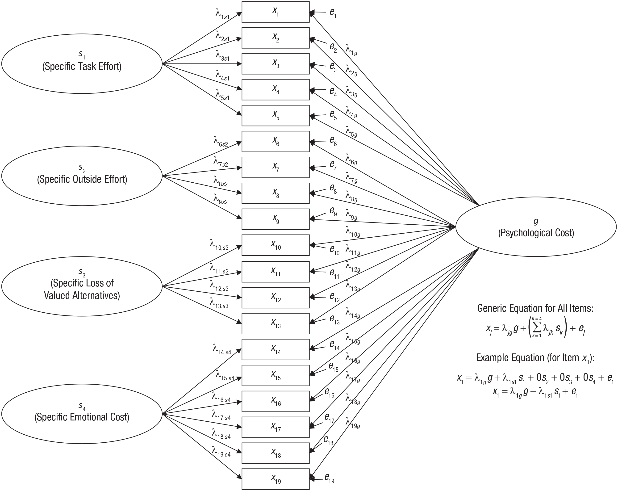
Bifactor model for the psychological-cost scale. See the text for further explanation.

Omega-hierarchical

When item-response data are well represented by a bifactor model, a reliability measure known as omega-hierarchical (or ω_h) represents the proportion of total-score variance due to a single, general construct that influences all items, despite the multidimensional nature of the item set (Rodriguez, Reise, & Haviland, 2016; Zinbarg et al., 2005). Just as the parameter estimates from a one-factor model are used to estimate reliability with ω_u, parameter estimates from a bifactor model are used to calculate ω_h, the formula of which is in Table 1. This formula for ω_h is like that for ω_u, except that the numerator is a function of the general-factor loadings only; the denominator again represents the estimated variance of the total score X. Therefore, ω_h represents the extent to which the total score provides a reliable measure of a construct represented by a general factor that influences all items in a multidimensional scale over and above extraneous influences captured by the specific factors.

Although several prominent resources have presented ω_h and discussed its conceptual advantages for estimating reliability of total scores from multidimensional tests (e.g., McDonald, 1999; Revelle & Zinbarg, 2009; Rodriguez et al., 2016; Zinbarg et al., 2005), little research has studied the finite-sample properties of ω_h estimates. Notably, Zinbarg et al. (2006) showed that ω_h estimates calculated using the CFA method described here are largely unbiased and are more accurate reliability estimates than alpha, showing trivial effects of design factors including the magnitude and heterogeneity of factor loadings, variation in sample size ranging from 50 to 200, the number of items, the number of specific factors, and the presence of cross-loadings. Yet no research to date has directly addressed whether ω_h estimates are robust to model misspecification (e.g., incorrectly using a bifactor model for a test with a different multidimensional structure).

As with ω_u, when the bifactor model is fitted to polychoric correlations among ordered, categorical items, applying the formula for ω_h leads to a reliability estimate in the x* latent-response-variable metric rather than the metric of the observed total score X. Instead, the approach of Green and Yang (2009b) can be applied to produce a version of ω_h that gives a reliability estimate of the proportion of total observed score variance due to the general factor; this estimate is referred to as ω_h-cat. Although ω_h-cat is not presented in Table 1, its equation is simply an adaptation of the equation for ω_u-cat in which the loadings from the one-factor model are replaced with general-factor loadings from a bifactor model.

Example calculation of ω_h in R

To demonstrate the estimation of ω_h using R, I use data my colleagues and I collected administering the PCS to 154 students in an introductory statistics course (Flake, Ferland, & Flora, 2017). With these data, alpha for the PCS total score is .96, but this may be a misleading reliability estimate because of multidimensionality; that is, alpha is a function of total variance due to all systematic influences on the items (i.e., both general and specific factors) rather than a measure of how reliably the total score measures a single target construct represented by a general factor. I fitted the bifactor model depicted in Figure 3 to the item-response data, treating the item responses as continuous variables because they were given on a 6-point scale.

The syntax to specify the bifactor model for lavaan is

> modBf <- ‘gen =~ TE1+TE2+TE3+TE4+TE5+OE1+OE2+OE3+OE4+LVA1+LVA2+LVA3+LVA4

+EM1+EM2+EM3+EM4+EM5+EM6

s1 =~ TE1 + TE2 + TE3 + TE4 + TE5

s2 =~ OE1 + OE2 + OE3 + OE4

s3 =~ LVA1 + LVA2 + LVA3 + LVA4

s4 =~ EM1 + EM2 + EM3 + EM4 + EM5 + EM6’

where gen is the general cost factor measured by all 19 items (i.e., TE1 through EM6), s1 is the specific factor for items pertaining to task-effort content (TE1 through TE5), s2 is the specific factor for items pertaining to outside-effort content (OE1 through OE4), s3 is the specific factor for loss-of-valued-alternatives items (LVA1 through LVA4), and s4 is the specific factor for emotional-cost items (EM1 through EM6). The model is estimated with

> fitBf <- cfa(modBf, data=pcs, std.lv=T, estimator=‘MLR’, orthogonal=T)

where the orthogonal=TRUE option forces all interfactor correlations to equal 0, which, as discussed earlier, is important for identification of bifactor models.

The results from the summary function indicate that the bifactor model fits the PCS data well, with robust model-fit statistics, CFI = .98, TLI = .97, RMSEA = .05. Thus, it is reasonable to calculate ω_h to estimate how reliably the PCS total score measures the general psychological-cost factor. Applying semTools::reliability to this fitted model,

> reliability(fitBf),

produces the following output: gen s1 s2 s3 s4 alpha 0.9638781 0.92504205 0.8992820 0.9052459 0.9405882 omega 0.9741033 0.56377307 0.7884791 0.6766430 0.7816839 omega2 0.9094893 0.09237594 0.3666293 0.1880759 0.2054075 omega3 0.9077636 0.09240479 0.3666634 0.1878380 0.2053012 avevar NA NA NA NA NA

Estimates listed under the gen column pertain to the general cost factor. The omega estimate, .97, ignores the contribution of the specific factors to calculation of the implied variance of the total score in its denominator (Jorgensen et al., 2020); thus, this value is not a reliability estimate for the PCS total score. Instead, the omega2 and omega3 values under gen are ω_h estimates; omega2 is calculated using the model-implied variance of the total score in its denominator, and omega3 is calculated using the observed sample variance of X (this distinction is analogous to the one between omega2 and omega3 described earlier for ω_u). Thus, the proportion of PCS total-score variance that is due to a general psychological cost factor over and above the influence of effects that are specific to the different content domains is .91.¹¹ Interpretation of the estimates listed under the s1 to s4 columns is described in the online supplement.

Higher-order models

In this bifactor-model example, I considered multidimensionality among the PCS items a nuisance for the measurement of a broad, general psychological-cost target construct. In other situations, researchers may hypothesize an alternative multidimensional structure such that there is a broad, overarching construct indirectly influencing all items in a test through more conceptually narrow constructs that directly influence different subsets of items. Such hypotheses imply that the item-level data arise from a higher-order model, in which a higher-order factor (also known as a second-order factor) causes individual differences in several more conceptually narrow lower-order factors (or first-order factors), which in turn directly influence the observed item responses. In this context, researchers may evaluate the extent to which the test produces reliable total scores (as measures of the construct represented by the higher-order factor) as well as subscale scores (as measures of the constructs represented by the lower-order factors).

When item scores arise from a higher-order model, a reliability measure termed omega-higher-order, or ω_ho, represents the proportion of total-score variance that is due to the higher-order factor; parameter estimates from a higher-order model are used to calculate ω_ho. As does ω_h, ω_ho represents the reliability of a total score for measuring a single construct that influences all items, despite the multidimensional nature of the test. Thus, the conceptual distinction between ω_h and ω_ho owes to the subtle difference between the interpretation of the general factor in the bifactor model and the higher-order factor in the higher-order model: In short, whereas the bifactor model’s general factor influences all items directly (while the specific factors are held constant), a higher-order factor influences all items indirectly via the lower-order factors (see Yung et al., 1999, for further detail). The online supplement to this article presents a formula for ω_ho and demonstrates the estimation of a higher-order model for the PCS and subsequent calculation of ω_ho as a function of the model’s parameter estimates. When the semTools::reliability function is applied to a fitted higher-order model, it does not return ω_ho; instead, the reliabilityL2 function of the semTools package calculates ω_ho, as shown in the online supplement, which also describes reliability estimation for subscales.¹²

Exploratory Omega Estimates

The examples presented thus far used semTools::reliability (or reliabilityL2) to estimate forms of omega from the results of CFA models. However, these estimates depend on correct specification of the model underlying a given test (e.g., ω_u is not an appropriate reliability estimate if the population model is multidimensional, as evidenced by poor fit of a one-factor model). When no hypothesized CFA model fits the data (as may be particularly likely in the early stages of test development), EFA can be used to help uncover a test’s dimensional structure. Once the optimal number of factors underlying a test is determined, the omega function from the psych package (Revelle, 2020) can be used to obtain an omega estimate based on EFA model parameters; this omega estimate will represent the proportion of total-score variance due to a general factor common to all items (see the online supplement for further discussion and a demonstration of this omega function).

Conclusion

Researchers should not mechanistically report alpha and instead should investigate the internal dimensional structure of a test to choose an appropriate reliability estimate for the measurement of a construct of interest, that is, an appropriate form of coefficient omega. This Tutorial has described alternative forms of omega that depend on a test’s underlying factor structure. Examples have been presented to demonstrate how to compute different omega estimates in R, mainly using semTools::reliability, which works on a CFA model fitted to the item-level data using the lavaan package.

The flowchart in Figure 4 summarizes recommendations for choosing an appropriate omega estimate; this chart applies to a situation in which a test is intended to measure a construct that is common to all items. The dimensional structure of the test determines the appropriate form of omega: ω_u (or ω_u-cat if the item responses are categorical) is appropriate for a unidimensional test (i.e., the item-response data conform to a one-factor model), and ω_h or ω_ho (or the categorical-variable analogue) is appropriate for the reliability of a total score calculated from a multidimensional item set conforming to a bifactor or higher-order model, respectively. If the test is multidimensional but a suitable CFA model cannot be hypothesized or does not adequately fit the data, then an EFA approach can be used both to discover potential reasons for multidimensionality and to obtain a preliminary, exploratory omega estimate.

Fig. 4.

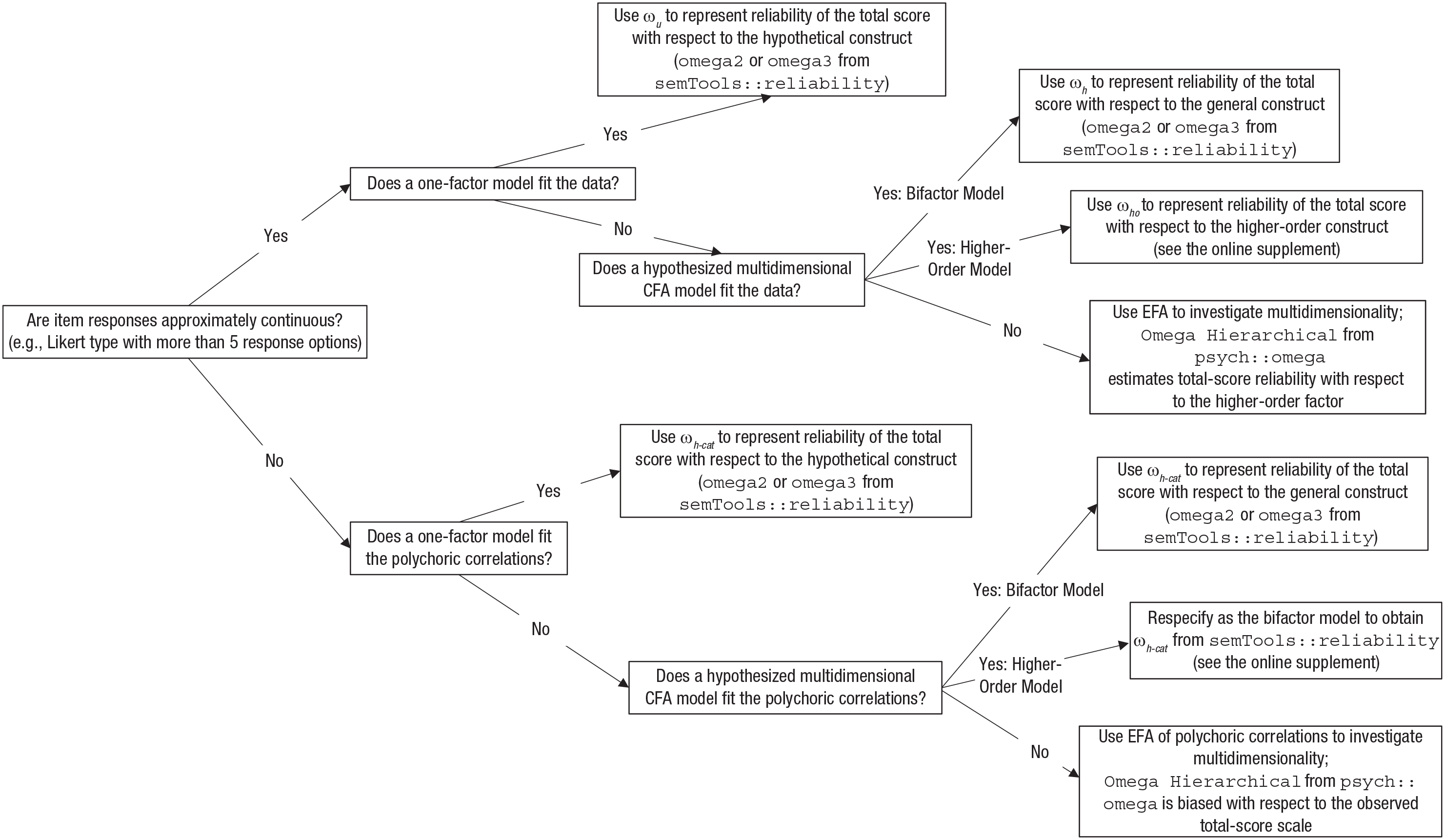
Flowchart for determining the appropriate omega estimate for measurement of a hypothetical construct influencing all items in a scale. CFA = confirmatory factor analysis; EFA = exploratory factor analysis.

An important issue often overlooked is that item responses typically have a categorical scale; therefore, deciding whether to treat the data as categorical (i.e., by fitting the factor model to polychoric correlations) affects both model-fit statistics and parameter estimates used to calculate omega estimates. Furthermore, Green and Yang (2009b) showed that when the measurement model is fitted to polychoric correlations, it is necessary to rescale the model’s parameter estimates to obtain reliability estimates in the metric of the observed total-score scale instead of a latent-response scale; ω_u-cat is an appropriate substitute for ω_u in this situation.

Although the essential tau-equivalence model underlying alpha is unlikely to be correct for a given test, it is also important for an omega estimate to be based on a properly specified measurement model, which highlights the importance of model comparisons and replication for evaluating a test’s internal structure (using factor analysis) and ultimately estimating the reliability of its scores. Further research is needed to examine the finite-sample properties of different omega estimates under correct model specification as well as their robustness to model misspecification, especially for multidimensional cases. Nevertheless, the extant studies clearly support a general preference for omega estimates over alpha (e.g., Trizano-Hermosilla & Alvarado, 2016; Yang & Green, 2010; Zinbarg et al., 2006). Yet, just as researchers should not blindly report alpha for the reliability of a test, they should not thoughtlessly report an omega coefficient without first investigating the test’s internal structure. The main conceptual benefit of using an omega coefficient to estimate reliability is realized when omega is based on a thoughtful modeling process that focuses on how well a test measures a target construct. Moving beyond mindless reliance on coefficient alpha and giving more careful attention to measurement quality is an important aspect of overcoming the replication crisis.

Supplemental Material

Flora_AMPPSOpenPracticesDisclosure – Supplemental material for Your Coefficient Alpha Is Probably Wrong, but Which Coefficient Omega Is Right?: A Tutorial on Using R to Obtain Better Reliability Estimates

Supplemental material, Flora_AMPPSOpenPracticesDisclosure for Your Coefficient Alpha Is Probably Wrong, but Which Coefficient Omega Is Right?: A Tutorial on Using R to Obtain Better Reliability Estimates by David B. Flora in Advances in Methods and Practices in Psychological Science

Footnotes

Acknowledgements

I would like to thank Reviewer 3 for detailed and constructive guidance across several drafts of this manuscript.

Transparency

Action Editor: Mijke Rhemtulla

Editor: Daniel J. Simons

Author Contributions

D. B. Flora is the sole author of this manuscript and is responsible for its content.

ORCID iD

David B. Flora

Notes

References

Bentler

P. M.

(2009). Alpha, dimension-free, and model-based internal consistency reliability. Psychometrika, 74, 137–143.

Bollen

K. A.

(1989). Structural equations with latent variables. New York, NY: Wiley.

Borsboom

(2005). Measuring the mind: Conceptual issues in contemporary psychometrics. New York, NY: Cambridge University Press.

Brown

T. A.

(2015). Confirmatory factor analysis for applied research (2nd ed.). New York, NY: Guilford Press.

Chalmers

R. P.

(2018). On misconceptions and the limited usefulness of ordinal alpha. Educational and Psychological Measurement, 78, 1056–1071.

Cole

Preacher

(2014). Manifest variable path analysis: Potentially serious and misleading consequences due to uncorrected measurement error. Psychological Methods, 19, 300–315.

Cronbach

L. J.

(1951). Coefficient alpha and the internal structure of tests. Psychometrika, 16, 297–334.

Eccles

J. S.

(2005). Subjective task value and the Eccles et al. model of achievement-related choices. In Elliot

A. J.

Dweck

C. S.

(Eds.), Handbook of competence and motivation (pp. 105–121). New York, NY: Guilford Press.

Finney

S. J.

DiStefano

(2013). Nonnormal and categorical data in structural equation modeling. In Hancock

G. R.

Mueller

R. O.

(Eds.), A second course in structural equation modeling (2nd ed., pp. 439–492). Charlotte, NC: Information Age.

10.

Flake

J. K.

Barron

K. E.

Hulleman

McCoach

B. D.

Welsh

M. E.

(2015). Measuring cost: The forgotten component of expectancy-value theory. Contemporary Educational Psychology, 41, 232–244.

11.

Flake

J. K.

Ferland

Flora

D. B.

(2017, April). Trajectories of psychological cost in gatekeeper classes: Relationships with expectancy, value, and performance. Paper presented at the annual meeting of the American Educational Research Association, San Antonio, TX.

12.

Flake

J. K.

Pek

Hehman

(2017). Construct validation in social and personality research: Current practice and recommendations. Social Psychological and Personality Science, 8, 370–378.

13.

Flora

D. B.

Flake

J. K.

(2017). The purpose and practice of exploratory and confirmatory factor analysis in psychological research: Decisions for scale development and validation. Canadian Journal of Behavioural Science, 49, 78–88.

14.

Flora

D. B.

LaBrish

Chalmers

R. P.

(2012). Old and new ideas for data screening and assumption testing for exploratory and confirmatory factor analysis. Frontiers in Psychology, 3, Article 55. doi:10.3389/fpsyg.2012.00055

15.

Fried

E. I.

Flake

J. K.

(2018). Measurement matters. Observer, 31(3), pp. 29–30.

16.

Green

S. B.

Yang

(2009a). Commentary on coefficient alpha: A cautionary tale. Psychometrika, 74, 121–135.

17.

Green

S. B.

Yang

(2009b). Reliability of summed item scores using structural equation modeling: An alternative to coefficient alpha. Psychometrika, 74, 155–167.

18.

Jonason

Webster

(2010). The dirty dozen: A concise measure of the dark triad. Psychological Assessment, 22, 420–432.

19.

Jöreskog

K. G.

(1971). Statistical analysis of sets of congeneric tests. Psychometrika, 36, 109–133.

20.

Jorgensen

T. D.

Pornprasertmanit

Schoemann

A. M.

Rosseel

(2020). semTools: Useful tools for structural equation modeling (R package Version 0.5-3) [Computer software]. Retrieved from https://CRAN.R-project.org/package=semTools

21.

Kelley

(2019). MBESS: The MBESS R package (R package Version 4.6.0) [Computer software]. Retrieved from https://CRAN.R-project.org/package=MBESS

22.

Kelley

Pornprasertmanit

(2016). Confidence intervals for population reliability coefficients: Evaluation of methods, recommendations, and software for composite measures. Psychological Methods, 21, 69–92.

23.

Loken

Gelman

(2017). Measurement error and the replication crisis: The assumption that measurement error always reduces effect sizes is false. Science, 355, 584–585.

24.

Lord

F. M.

Novick

M. R.

(1968). Statistical theories of mental test scores. Reading, MA: Addison-Wesley.

25.

McDonald

R. P.

(1999). Test theory: A unified approach. Mahwah, NJ: Erlbaum.

26.

McNeish

(2018). Thanks coefficient alpha, we’ll take it from here. Psychological Methods, 23, 412–433.

27.

Mellenbergh

G. J.

(1996). Measurement precision in test score and item response models. Psychological Methods, 1, 293–299.

28.

R Core Team. (2018). R: A language and environment for statistical computing. Vienna, Austria: R Foundation for Statistical Computing.

29.

Revelle

(2020). psych: Procedures for psychological, psychometric, and personality research (R package Version 2.0.9) [Computer software]. Retrieved from https://cran.r-project.org/web/packages/psych/index.html

30.

Revelle

Condon

D. M.

(2019). Reliability from α to ω: A tutorial. Psychological Assessment, 31, 1395–1411.

31.

Revelle

Wilt

Rosenthal

(2010). Individual differences in cognition: New methods for examining the personality-cognition link. In Gruszka

Matthews

Szymura

(Eds.), Handbook of individual differences in cognition: Attention, memory and executive control (pp. 27–49). New York, NY: Springer.

32.

Revelle

Zinbarg

R. E.

(2009). Coefficients alpha, beta, omega, and the glb: Comments on Sijtsma. Psychometrika, 74, 145–154.

33.

Rhemtulla

Brosseau-Liard

P. E.

Savalei

(2012). When can categorical variables be treated as continuous? A comparison of robust continuous and categorical SEM estimation methods under suboptimal conditions. Psychological Methods, 17, 354–373.

34.

Rodriguez

Reise

S. P.

Haviland

M. G.

(2016). Evaluating bifactor models: Calculating and interpreting statistical indices. Psychological Methods, 21, 137–150.

35.

Rosseel

(2012). lavaan: An R package for structural equation modeling. Journal of Statistical Software, 48(2).

36.

Savalei

(2018). On the computation of the RMSEA and CFI from the mean-and-variance corrected test statistic with nonnormal data in SEM. Multivariate Behavioral Research, 53, 419–429.

37.

Savalei

(2019). A comparison of several approaches for controlling measurement error in small samples. Psychological Methods, 24, 352–370.

38.

Savalei

Reise

S. P.

(2019). Don’t forget the model in your model-based reliability coefficients: A reply to McNeish (2018). Collabra: Psychology, 5, Article 36. doi:10.1525/collabra.247

39.

Sijtsma

(2009). On the use, the misuse, and the very limited usefulness of Cronbach’s alpha. Psychometrika, 74, 107–120.

40.

Trizano-Hermosilla

Alvarado

J. M.

(2016). Best alternatives to Cronbach’s alpha reliability in realistic conditions: Congeneric and asymmetrical measurements. Frontiers in Psychology, 7, Article 769. doi:10.3389/fpsyg.2016.00769

41.

Wirth

R. J.

Edwards

M. C.

(2007). Item factor analysis: Current approaches and future directions. Psychological Methods, 12, 58–79.

42.

Yang

Green

S. B.

(2010). A note on structural equation modeling estimates of reliability. Structural Equation Modeling, 17, 66–81.

43.

Yang

Green

S. B.

(2015). Evaluation of structural equation modeling estimates of reliability for scales with ordered categorical items. Methodology, 11, 23–34.

44.

Yung

Y.-F.

Thissen

McLeod

L. D.

(1999). On the relationship between the higher-order factor model and the hierarchical factor model. Psychometrika, 64, 113–128.

45.

Zinbarg

R. E.

Revelle

Yovel

(2005). Cronbach’s α, Revelle’s β, and McDonald’s ωh: Their re-lations with each other and two alternative conceptualizations of reliability. Psychometrika, 70, 123–133.

46.

Zinbarg

R. E.

Yovel

Revelle

McDonald

R. P.

(2006). Estimating generalizability to a latent variable common to all of a scale’s indicators: A comparison of estimators for ω_h. Applied Psychological Measurement, 30, 121–144.

47.

Zumbo

B. D.

Gadermann

A. M.

Zeisser

(2007). Ordinal versions of coefficients alpha and theta for Likert rating scales. Journal of Modern Applied Statistical Methods, 6, 21–29.

48.

Zumbo

B. D.

Kroc

(2019). A measurement is a choice and Stevens’ scales of measurement do not help make it: A response to Chalmers. Educational and Psychological Measurement, 79, 1184–1197.

Supplementary Material

Please find the following supplemental material available below.

For Open Access articles published under a Creative Commons License, all supplemental material carries the same license as the article it is associated with.

For non-Open Access articles published, all supplemental material carries a non-exclusive license, and permission requests for re-use of supplemental material or any part of supplemental material shall be sent directly to the copyright owner as specified in the copyright notice associated with the article.

0.00 MB

0.64 MB

Your Coefficient Alpha Is Probably Wrong,but Which Coefficient Omega Is Right? A Tutorial on Using R to Obtain Better Reliability Estimates

Abstract

Keywords

Disclosures

What Is Reliability?

Reliability of Unidimensional Tests: Omega to Alpha

Coefficient omega

Coefficient alpha

Example calculation of ω u in R

Factor Analysis of Ordered, Categorical Items

Categorical omega

Example calculation of ω u-cat in R

Reliability Estimates for Multidimensional Scales

Bifactor models

Omega-hierarchical

Example calculation of ω h in R

Higher-order models

Exploratory Omega Estimates

Conclusion

Supplemental Material

Flora_AMPPSOpenPracticesDisclosure – Supplemental material for Your Coefficient Alpha Is Probably Wrong, but Which Coefficient Omega Is Right?: A Tutorial on Using R to Obtain Better Reliability Estimates

Footnotes

Acknowledgements

Transparency

ORCID iD

Notes

References

Supplementary Material

Example calculation of ω_u in R

Example calculation of ω_u-cat in R

Example calculation of ω_h in R