Sage Journals: Discover world-class research

Abstract

Cross-validation is a statistical procedure that every psychologist should know. Most are possibly familiar with the procedure in a global way but have not used it for the analysis of their own data. We introduce cross-validation for the purpose of model selection in a general sense, as well as an R package we have developed for this kind of analysis, and we present examples illustrating the use of this package for types of research problems that are often encountered in the social sciences. Cross-validation can be an easy-to-use alternative to null-hypothesis testing, and it has the benefit that it does not make as many assumptions.

Keywords

predictive accuracy reproducibility cross-validation prediction

The simple idea of splitting a sample into two and then developing the hypothesis on the basis of one part and testing it on the remainder may perhaps be said to be one of the most seriously neglected ideas in statistics.

—G. A. Barnard (commentary in Stone, 1974, p. 133)

Null-hypothesis significance testing is still the dominant paradigm in psychological research despite numerous rounds of debate (Chow, 1998; Cohen, 1994; Hagen, 1997; Krueger, 2001; Nickerson, 2000; Rozeboom, 1960). The many alternatives that have been proposed include a focus on estimation and confidence intervals (Cumming, 2014) and a Bayesian approach (see Wagenmakers, 2007). A particularly intriguing sentence in Wagenmakers’s (2007) discussion of the latter alternative reads as follows: “The universal yardstick for selecting between competing models is predictive performance” (p. 795). In this Tutorial, we follow this lead of focusing on predictive performance in a cross-validation framework.

Since early this century, there has been an increased interest in prediction, as opposed to explanation (Breiman, 2001; Shmueli, 2010). Explanatory data analysis starts with a theory about an empirical phenomenon. The statistical model is a translation of the theory into mathematical form, and statistical inference (tests, standard errors, p values) is used to test the theory. The parameters of the model—for example, the regression weights in a multiple regression model—are its key elements because they provide the test of the theory.

In contrast, in the predictive approach, the model itself is not of great interest, but the predictions the model generates are. In other words, to continue our previous example, the regression weights of a multiple regression model are not of interest, but the predictions that the regression model makes are. (For a recent discussion of the distinction between the inferential and prediction approaches in psychology, see Yarkoni & Westfall, 2017. More statistical treatments can be found in Breiman, 2001, and Shmueli, 2010.)

The theory underlying predictive models rests on the trade-off between bias and variance. Simply stated, the more complex a model is (i.e., the more parameters it includes), the better it will fit the data (less bias), but the more variable its predictions will be (more variance). On the other hand, a simpler model will fit worse (more bias), but its predictions will be less variable (less variance). In a formal sense, when one fits a statistical model to a sample of data and investigates its predictive performance, the expected prediction error decomposes into (squared) bias and variance of the fitted model (Hastie, Tibshirani, & Friedman, 2009). The bias represents how far the average estimated model is from the true population model, whereas the variance represents the variability of the estimated models from sample to sample (for a detailed mathematical treatment, see Hastie et al., 2009, and Matloff, 2017; more narrative treatments specific to psychology can be found in Yarkoni & Westfall, 2017; Chapman, Weiss, & Duberstein, 2016; and McNeish, 2015). Trading off bias and variance in practical data analysis is often performed through cross-validation.

In its early years, the psychometric literature already included a substantial amount of work on trading off bias and variance, most notably through simple weighting schemes for regression (Lawshe & Schucker, 1959; Pruzek & Frederick, 1978; Schmidt, 1971; Wainer, 1976), but also through estimating shrunken regression weights (Darlington, 1978; Rozeboom, 1979). Both methods allow for bias in the regression equation (simple unit weights or shrunken weights will, on average, not be equal to the population weights) in order to reduce the variance (i.e., unit weights do not depend on the data and therefore have zero variance).

It is often claimed that ordinary least squares regression produces unbiased estimates of the population model’s parameters. This sounds reassuring but is generally false. The claim should be that if the assumptions of regression are true, ordinary least squares regression produces unbiased estimates. This is an important qualification that has been at the center of a great deal of confusion because, in general, the assumptions of a linear regression model are not strictly true, and the regression coefficients might therefore be biased. For example, if the relationship between two variables is nonlinear in the population, ordinary least squares linear regression cannot be correct on average.

The goal of explanatory modeling is to identify the true, unbiased model, so that a theory can be tested, whereas the goal of predictive modeling is to identify false (biased) but stable models. A researcher who wants to test whether a coefficient in the true underlying probability model equals zero should use a statistical test resulting in a p value, because cross-validation does not consistently find the true underlying model. Whereas p values test the hypothesis that an effect is zero in the population, cross-validation tests whether a model’s predictions become better if this effect is added to the model. Hagerty and Srinivasan (1991) showed that including true but small effects in a statistical model does not always make predictions better.

In the early days of psychometrics, there was quite strong interest in cross-validation of regression equations (Mosier, 1951). The motivation was that the explained variance for the sample used to develop a regression model will to some extent reflect model overfit and be too high. A better estimate of explained variance therefore comes from a new sample that is entirely independent of the development sample. Mosier (1951) was the first to propose something like what is nowadays often referred to as two-sample cross-validation, that is, fitting a regression model in the first sample and validating it in the second, fitting the model in the second sample and validating it in the first, and then taking the average of the two obtained correlations as the final cross-validation coefficient. Alternatively, there are statistical adjustments that one can make to estimate cross-validation results (see, e.g., Darlington, 1968; Rozeboom, 1978; and Claudy, 1978).

There are advantages to both approaches. The two-sample cross-validation approach requires no distributional assumptions (Browne, 2000), but the formula-adjustment approach uses the data more efficiently. That is, two-sample cross-validation is inefficient in the sense that both the calibration (or training) set and the validation (or test) set are much smaller than the complete data set. Therefore, the estimation is not as efficient as it could be, and the validation set is small. Stone (1974) and Geisser (1975) tried to alleviate both concerns by introducing leave-one-out cross-validation, in which the data for N – 1 persons are used to estimate a model, and the data for 1 person are used to validate it, and this procedure is repeated until every observation has been used as the validation sample. Because the training samples are almost as large as the complete data set, much more efficient use is made of the data.

All these approaches use cross-validation to assess one final regression equation, that is, a model that has been obtained from the data in some way, say, by using p values. In machine learning, cross-validation is most often used for evaluation of different modeling procedures and for variable or model selection. In the case of model selection, every model under consideration is cross-validated, and the one with the smallest prediction error (i.e., loss) is selected. Such a procedure might be useful for psychological research but has not often been used by psychologists. One of the reasons might be that psychological researchers do not know how to perform such cross-validation, as there is no standard statistical software routine available for performing it. SPSS, for example, does not have a cross-validation tool, nor does it have the capability of fitting a regression model on part of the data and using the fitted model to make predictions for another part of the data.

The goal of this Tutorial is to provide a rough outline of cross-validation for model selection, to introduce easily usable software (an R package) we have developed for this purpose, and to present a set of empirical examples. We conclude with a discussion on the use of the R package, the difficulties of model selection in general, and the relationship between our cross-validation procedure and other forms of cross-validation.

Cross-Validation: Theory and an R Package

The oldest and simplest way to perform cross-validation is independent verification, in which one has two independent data sets: a calibration set (C) and a validation set (V). The observations in the calibration set can be indexed with i = 1, . . . N_C, and those in the validation set with j = 1, . . . N_V.

In the calibration set, one fits the statistical model, for example, y_i = a + b^T x_i + e_i, to obtain estimated parameters $\hat{a}$ and $\hat{b}$ . In the validation set, one uses the estimated parameters and the values of the predictor variables (x_j) to compute predictions: ${\hat{y}}_{j}$ = $\hat{a}$ + ${\hat{b}}^{T}$ x_j. The predicted values ${\hat{y}}_{j}$ are used to compute the root mean square error of prediction (RMSE_p):

R M S E_{p} = \sqrt{\frac{1}{N_{V}} \sum_{j = 1}^{N_{V}} {(y_{j} - {\hat{y}}_{j})}^{2}} .

In R (R Core Team, 2018), one can easily fit a model on the calibration set using the following code to obtain the estimated parameters:

output = glm(y ~ x, data = calibrationdata).

With the output of the model, one can make predictions for new data (i.e., the validation data) by using

predictions = predict(output, newdata = validationdata, type = “response”).

Finally, the root mean square error of prediction can be computed using

sqrt(mean((predictions - validationdata$y)^2)).

We deliberately focus on an unstandardized measure on the scale of the original response variable. Within a sample, there is a direct link between the mean square error and the explained variance. Out of that sample, however, this link is broken because the mean is not calibrated. Therefore, Model 1 might predict ${\hat{y}}_{j}$ = {1, 2, 3, 4, 5}, and Model 2 might predict ${\hat{y}}_{j}$ = {7, 8, 9, 10, 11}, when the actual observations in the validation set are y_j = {6, 7, 8, 9, 10}. It is clear that for both sets of predictions, the correlation with the observed outcome equals 1, whereas the RMSE_p equals 5 for the first set of predictions and 1 for the second set (for more details, see Alexander, Tropsha, & Winkler, 2015).

This Tutorial focuses on cross-validation for model selection. In this scenario, the researcher has two or more models of interest and is interested in determining which model is best. In cross-validation, “best” is operationalized as having the smallest root mean square error of prediction. Our focus is on models from the family of generalized linear models. Many standard analysis tools often used in psychology fall in this family; these include the one-sample and two-samples t test, one-way and multiway analysis of variance, (multiple) regression, analysis of covariance, and logistic regression. Furthermore, this family is easily enriched to develop nonlinear regression models using polynomials (as we show) or splines. (See, e.g., Fox, 2016, for the general framework that links these analytic techniques.)

An important disadvantage of independent verification is that one needs two data sets. A rather simple alternative to collecting two data sets is to collect only a single data set and then divide it into two independent sets. James, Witten, Hastie, and Tibshirani (2013) called this the validation-set approach to cross-validation. One part of the original data set takes the role of the calibration set, whereas the other takes the role of the validation set. As noted earlier, however, this strategy for performing cross-validation is not very efficient, because only half of the data is used to fit the model. Indeed, 70 years ago, Mosier (1951) already pointed to the loss of information in such an approach. However, the idea of splitting a data set into a calibration set and a validation set can be recycled: One can split the data into K independent sets of observations and use every set in turn as the validation set for which the other K – 1 sets are the calibration set. This is called K-fold cross-validation, and it leads to predictions for every observation in the data set. The data are thus used more efficiently. K is often chosen to be equal to 5 or 10 (see the section titled Choices to Be Made by the Researcher for further discussion about this choice). There are many ways in which the data can be partitioned into K sets, and each leads to a slightly different estimate of the root mean square error of prediction. To deal with these different estimates, it is necessary to repeat the cross-validation several times (Harrell, 2015). Using a large number of replications (also termed repeats) solves the problem that one model might be favored as a result of a particular partitioning into sets. Repeating the K-fold cross-validation a number of times also has the advantage that one can count the number of times a particular model wins, that is, the number of times that model has a smaller prediction error than the other models under investigation.

We have implemented these ideas in the R package xvalglms. The main function in this package, xval.glm, performs repeated K-fold cross-validation on a set of models. The user first needs to define a list of models and then calls the xval.glm function. Suppose you have a single predictor variable x and a response variable y, and you would like to know whether predictions become more accurate if you use the predictor variable. You can compare the prediction errors of a model with and without the predictor variable as follows:

models <- vector(mode = “list”, length = 2)

models[[1]] <- y ~ 1

models[[2]] <- y ~ 1 + x

output <- xval.glm(data = mydata, models)

This example specifies two regression models: Model 1, with only an intercept (i.e., without the predictor variable), and Model 2, with an intercept and the predictor.

The function outputs the following information, along with a graph:

Results for (10-fold, 200 repeats)

[ 1] y ~ 1 | 0% | 0.409 | 0.412 | 0.418 |

[ 2] y ~ 1 + x | 100% | 0.394 | 0.401 | 0.410 |

For each model, the output shows the percentage of times it yields the smallest of the prediction errors from the models in competition (“wins” column), its average prediction error (“mean” column), and the 95% confidence bounds for its prediction error (“2.5%” and “97.5%” columns).

The default graph has three panels (see Fig. 1). The upper panel shows the cumulative proportion of wins for each model during the repeated cycles of 10-fold cross-validation and can be used to verify whether the cross-validation results stabilized. If the lines are not flat at the end, the researcher should ask for more repeats of the K-fold cross-validation. The panel directly below shows boxplots of the 200 repetitions of prediction error. The panel on the right shows a density estimate for the boxplots. All this information is returned in an output object that can be saved.

Fig. 1.

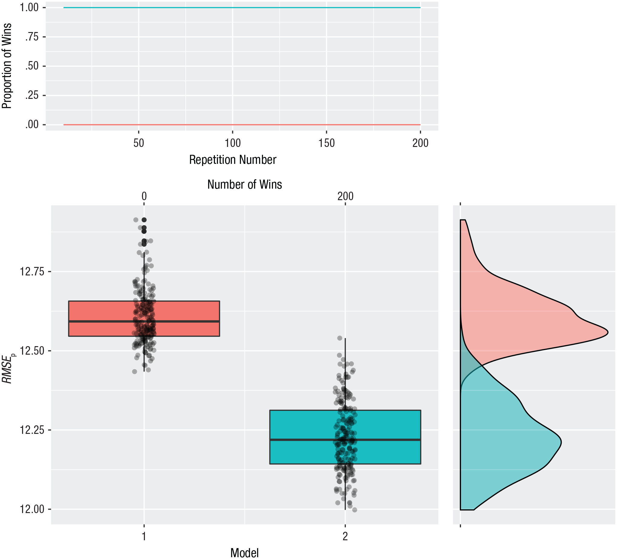
Illustration of the output of the xvalglms package for a two-model comparison with 200 repetitions of 10-fold cross-validation. The upper panel shows the proportion of wins for each model as a function of the repetition number. The panel directly below shows boxplots of the two models’ prediction error (root mean square error of prediction, RMSEp); each box indicates the middle 50% of values, the horizontal line inside the box indicates the median, and the vertical lines represent the range from lowest to highest prediction error, excluding outliers. The number of wins for each model is shown at the top. The panel on the right is a graph of the density estimates for the prediction errors of the competing models.

Assumptions

Many introductory statistics textbooks emphasize the assumptions of statistical techniques. For linear regression, for example, the most important assumptions are (a) a linear relationship between the explanatory variable and the response variable in the population, (b) normally distributed errors with constant variance (homoscedasticity), and (c) independence of the observations (Fox, 2016).

In the predictive mode, many of these standard assumptions are not needed any more. Focusing on the bias-variance trade-off is a strategy of actively seeking a bit of bias while diminishing variance. In that sense, there is no need to assume a linear relationship between the predictor and response variable; one can compare the predictive performance of several regression models, linear and nonlinear, and select one. The selected model is not necessarily equal to a true model (if that exists); it is the model that provides the best predictions as evaluated using the current data set. If the true population model is nonlinear but the optimal predictive model is linear, this means that the usual assumption of normally distributed residuals with constant variance is false. Therefore, one can conclude that such a distributional assumption for the residuals is not needed when one uses cross-validation for model selection.

However, the assumption that observations are independent remains. If the observations are not independent, the cross-validation procedure must be adapted to take into account the dependency. For clustered data (e.g., repeated measures within a participant or participants clustered in teams), a clustered variant of cross-validation might be employed (Roberts et al., 2016).

What is important in cross-validation is the loss function employed to compute prediction error. In our examples, we use the square root of the averaged squared difference between the predictions and the actual observations. We could have focused on other loss functions, such as the average absolute loss, which probably would have led to other models being identified as optimal. In one of our application examples in the next section (and in the Supplemental Material), we illustrate the use of other loss functions.

Choices to be made by the researcher

Users of the cross-validation procedure have to make several choices: They must choose the number of folds, the number of repetitions, the loss function, and which models to compare. In our R package, we set some default values, which were chosen wisely and which we explain here:

The choice of the number of folds is itself a bias-variance trade-off. With K equal to the number of observations in the sample, an almost unbiased estimate of the prediction error is obtained, because the size of the training sample in each of the folds is almost equal to the sample size. This absence of bias sounds good, but the variance from sample to sample is large. On the other hand, with K equal to 2, there is much less sample-to-sample variation, but the bias may be much larger because the training sample in each of the folds is only half of the sample size. Usually K = 10 is thought to be a good compromise, and we use it as default. When sample sizes are small—say, smaller than 40—we advise lowering K to, for example, 5.

Repetitions are important because they take away the randomness of results due to splitting the sample into K parts. Harrell (2015) advised using such repetitions. For our default, we chose a large number, 200. Because researchers nowadays have considerable computational power, this is not an issue. To evaluate whether 200 repetitions is enough, a researcher may look at the proportion of wins of each model over the repetitions (see, e.g., the top panel of Fig. 1). If the proportion of wins has stabilized, the researcher can be confident that the number is large enough. If there is still large variation, we suggest increasing the number of repetitions. Note that there is an interplay between the number of repetitions and the number of folds. If one uses leave-one-out cross-validation (K = sample size), there is no need to repeat the cross-validation because in every repetition exactly the same prediction error is estimated.

As we have mentioned, our default for the loss function is the root mean square error. This is a loss function that can be used for different type of distributions in generalized linear models. However, in certain circumstances, a researcher might want to change the loss function. If, for example, one needs to make a decision for individuals, such as selecting them for treatment or a job, it is sensible to change the loss function for the logistic regression model to the misclassification rate. Alternatively, one might want to use a more robust version of a loss function and could choose absolute error loss instead of squared error loss for linear regression models. In the next section, we show how to change the loss function and discuss the implications of the choice of loss function for the model-selection results.

The last choice a researcher needs to make is which models to compare. Ideally, one would like to include all possible models, but especially in cases with many variables, comparing all possible models is not an option. The choice of models to compare can be guided from a more data-driven or a more theory-driven perspective. From a data-driven perspective, a researcher could let the data decide which models to include; however, such approaches can easily lead to underestimation of prediction errors (Hastie et al., 2009). The current implementation of our cross-validation R package does not include this form of estimation. Taking a theory-driven perspective instead, a researcher has to choose which models to include. This can be done on the basis of, for example, theory or previous literature, but also on the basis of information regarding how likely certain models are. This latter option is akin to prior selection in a Bayesian framework, in which certain models are assigned less weight if they are highly unlikely. Note that these issues arise mainly when there is a very large set of possible models. The number of variables in most psychological experiments is small enough to allow all models to be tested with our current framework.

Applications of Cross-Validation

In this section, we present six applications of the cross-validation methodology. The first corresponds to a two-samples t test. The corresponding predictive question is whether the overall mean for the two groups or a separate mean for each group provides better prediction. In other words, does prediction become better if we use group information? The second application involves a univariate regression in which we would like to see whether the response variable is predicted better by using a predictor variable or by using the overall mean alone (i.e., an intercept-only model). Furthermore, we consider possible nonlinear relationships between the predictor and response variables by asking whether a second- or third-order polynomial predicts better than a linear regression does. Our third application concerns a complex regression situation in which we expect higher-order interaction effects. In our fourth example, we look at a univariate regression with a dichotomous outcome. In this logistic regression, we also compare polynomial models. The choice of the loss function in the cross-validation procedure can affect the results, and we illustrate this in our fifth example. In the sixth example, we compare two theories using cross-validation, in order to choose the theory that results in the most accurate predictions.

Before one can use the cross-validation function in xvalglms, it is necessary to download and load the package. This can be done as follows:

library(devtools)

install_github("Github-MS/xvalglms")

library(xvalglms)

Example 1: two-samples t test

The data set we use for this example is described in Howell’s (2015) textbook but originally came from Adams, Wright, and Lohr (1996). The authors were interested in the theory that homophobia may be unconsiously related to anxiety about being or becoming homosexual. They administered an index of homophobia to 64 heterosexual males, who were then classified as either homophobic or nonhomophobic according to their scores. The men than saw sexually explicit videos portraying homosexual and heterosexual behavior, and their sexual arousal was recorded. Adams et al. reasoned that if homophobia is unconsciously related to anxiety about one’s own sexuality, homophobic individuals would show greater arousal in response to homosexual videos than would nonhomophobic individuals.

The data for this example can be loaded from the Internet using

library(foreign)

mfile = “http://www.uvm.edu/~dhowell/methods8/DataFiles/Tab7-5.sav"

Arousal = read.spss(mfile, to.data.frame = TRUE)

This code puts the data in a data frame called Arousal.

In this example, we are interested in comparing predictions based on the overall mean with predictions based on the group means. We define these two models and then run our cross-validation function as follows:

models = vector(mode = “list”, length = 2)

models[[1]] = Arousal ~ 1

models[[2]] = Arousal ~ 1 + Group

output = xval.glm(data = Arousal, models)

This code specifies a model predicting arousal level on the basis of the intercept alone (Model 1) and a model predicting arousal on the basis of whether someone is homophobic or nonhomophobic (group; Model 2). Theoretically, the question that cross-validation will answer is whether adding the group variable leads to more accurate predictions of arousal than are achieved by predicting arousal from the overall mean arousal score only.

The output of this function is shown in Figure 2. Model 2 wins in all 200 cases and returns a much lower prediction error of around 12.20.

Fig. 2.

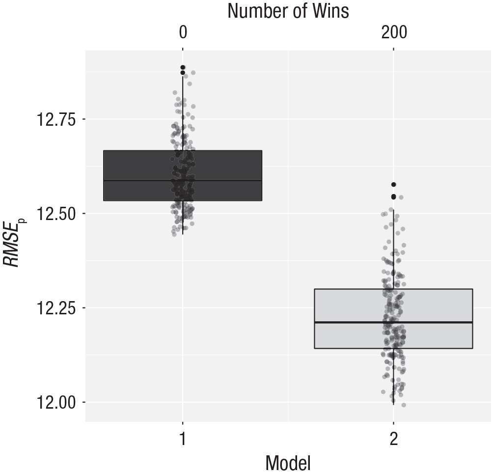
Cross-validation results for the arousal data. Model 1 makes predictions based on the overall mean; Model 2 makes predictions based on the group means. The vertical axis represents the root mean square error of prediction (RMSEp). The number of wins is represented at the top of the graph. See Figure 1 for an explanation of the conventions used in the boxplots.

The two means that we need to use for making future predictions are 24.00 for Group 1 (homophobic) and 16.50 for Group 2 (nonhomophobic). Predictions made using these means will be on average 12.20 units (RMSE_p) off from the true value. This is quite a lot of error, but less than occurs when only the overall mean is used to make predictions.

Example 2: linear regression

A general goal of a study conducted by Margolin and Medina, and described in Wilcox (2017, p. 223), was to examine how children’s information processing is related to a history of exposure to marital aggression. Data were collected from 47 children. The aggression variable in this study reflected physical, verbal, and emotional aggression the children experienced during the previous year, and their information processing was measured on a recall test. We first read in the data in the data frame agdat:

mfile = “https://dornsife.usc.edu/assets/sites/239/docs/

marital_agg_dat.txt"

agdat = read.table(mfile, header = TRUE)

A scatterplot of test score against aggression (see Fig. 3) shows a decreasing trend in which test scores go down as aggression increases, although some upward trend for values of aggression is visible.

Fig. 3.

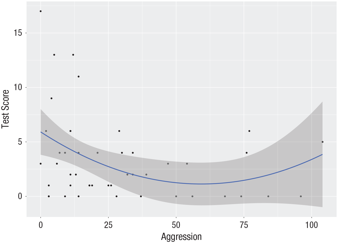
Scatterplot (with best-fitting regression line) of the aggression data: score on the recall test as a function of the aggression variable. The gray band represents uncertainty about the regression line (in the unlikely case that all assumptions are met, it represents the 95% confidence interval).

Next, we specify the theoretically relevant models:

models = vector(mode = “list”, length = 4)

models[[1]] = test ~ 1

models[[2]] = test ~ Aggression

models[[3]] = test ~ poly(Aggression,2)

models[[4]] = test ~ poly(Aggression,3)

output = xval.glm(data = agdat, models)

The first model in this case specifies only the mean (an intercept). The second model includes aggression as a predictor. The question that cross-validation answers is whether the inclusion of this predictor leads to more accurate out-of-sample predictions. In this example, we also include nonlinear models: a quadratic polynomial (Model 3) and a cubic polynomial (Model 4). With the last line of code, we call the cross-validation function to compare the predictive power of the four models. The results are shown in Figure 4. The quadratic model predicts best; that is, the prediction error is lower for the quadratic model than for the other models. Figure 3 shows the quadratic model fitted to the complete data. It is this model that might subsequently be used to interpret the relationship between aggression and score on the recall test.

Fig. 4.

Cross-validation results for the aggression data. Model 1 makes predictions based on the overall mean, Model 2 uses a first-order polynomial of aggression, Model 3 uses a second-order polynomial, and Model 4 uses a third-order polynomial. The vertical axis represents the root mean square error of prediction (RMSE_p). The number of wins is represented at the top of the graph. See Figure 1 for an explanation of the conventions used in the boxplots.

The standard approach to model selection would use change in explained variance and incremental F tests. The F tests and resulting p values require assumptions such as normally distributed error terms with a mean of zero and constant variance. In the Supplemental Material, we show this analysis but also show that the assumptions are not tenable. The conditional mean of the residuals is not always zero, and the distribution of the residuals is positively skewed. These might affect the test statistics. The cross-validation procedure does not make these assumptions.

Example 3: moderated regression

In this section, we use publicly available data from a study that examined the effects of mortality salience (M) on attitudes about Muslims and multiculturalism (A) among native Dutch people with varying levels of national identification (N) and self-esteem (S; Tjew-A-Sin & Koole, 2018a, 2018b). In their original study, the authors hypothesized and found a three-way interaction of mortality salience, national identification, and self-esteem. They also found a main effect of national identification, a main effect of self-esteem, and a marginal interaction between self-esteem and mortality salience.

Exploring the data, we found 5 participants with extreme scores on the national-identification and self-esteem scales. In the Supplemental Material, we present analyses with and without the data for these 5 participants. Here, for illustrative purposes, we report only on the data with the 5 participants removed. We note that the three-way interaction observed by Tjew-A-Sin and Koole (2018b) is still present in this cleaned data set.

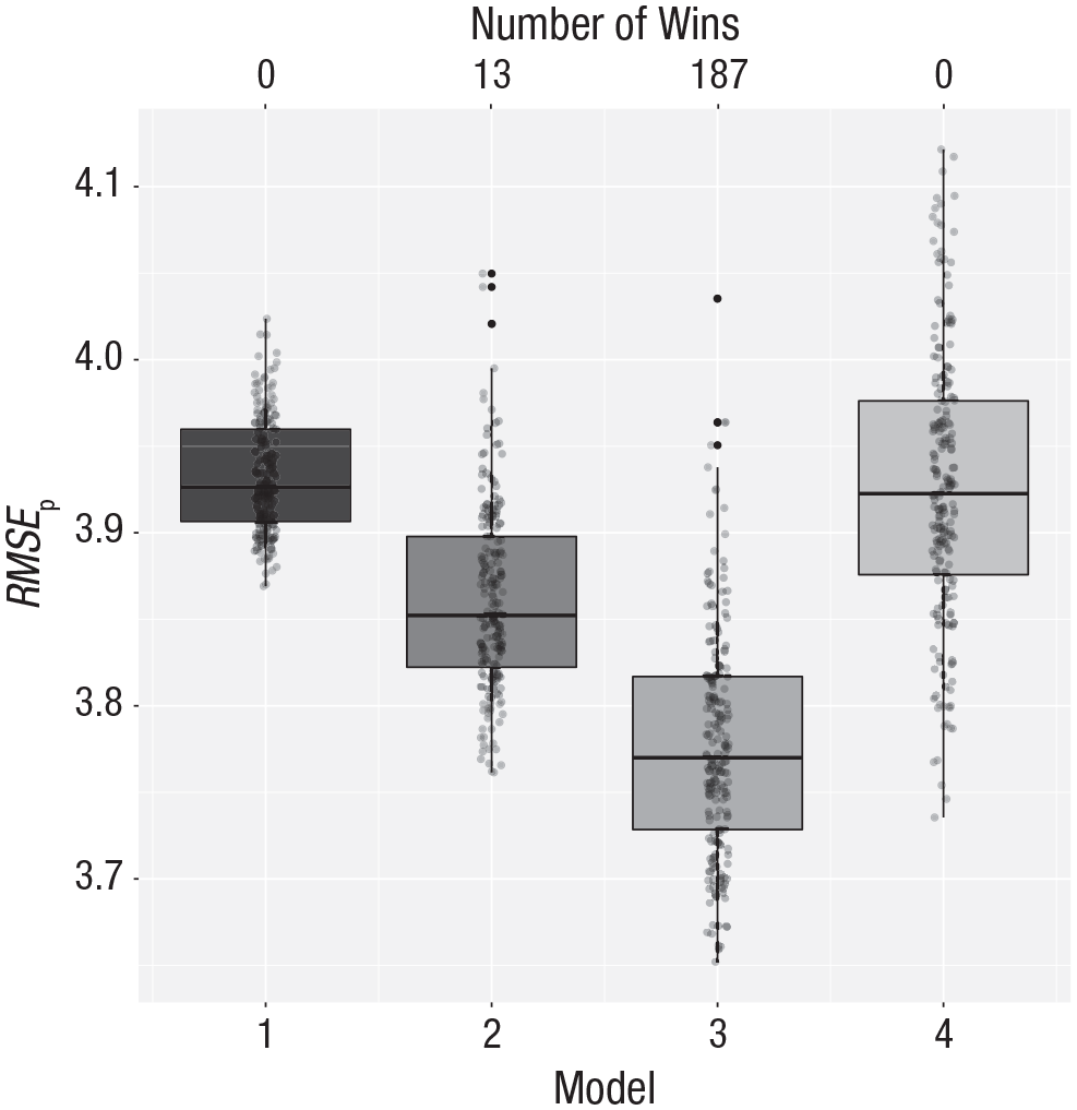
Whereas the authors used one complicated model and checked which effects were statistically significant, we approach this problem as a model-selection issue in which 16 different models are formulated. The simplest is the intercept-only model (Model 1), and the most complex is the one including all main effects, all two-way interactions, and the three-way interaction (Model 16):

models = vector(mode = “list”, length = 16)

models[[1]] = A ~ 1

models[[2]] = A ~ M

models[[3]] = A ~ N

models[[4]] = A ~ S

models[[5]] = A ~ M + S

models[[6]] = A ~ M + N

models[[7]] = A ~ S + N

models[[8]] = A ~ M + S + N

models[[9]] = A ~ M * S + N

models[[10]] = A ~ M + S * N

models[[11]] = A ~ M * N + S

models[[12]] = A ~ M * N + M * S

models[[13]] = A ~ M * N + N * S

models[[14]] = A ~ M * S + N * S

models[[15]] = A ~ M * S + N * S + M * N

models[[16]] = A ~ M * N * S

The results of this analysis are shown in Figure 5. There are four competing models: Model 3, with only a main effect of national identification (33% of the wins); Model 7, with main effects of self-esteem and national identification (10% of the wins); Model 9, with a two-way interaction between self-esteem and mortality salience and a main effect of national identification (16% of the wins); and Model 16, with the three-way interaction (42% of the wins). Although the latter model wins in 84 of the 200 repetitions, the average prediction error for this model is 0.667, whereas that of the model with only a main effect is 0.665, a little bit smaller. The other two competing models have a root mean square error of prediction of 0.667. Therefore, in terms of prediction all these model do equally well. The most complicated model has the widest 95% prediction interval, from 0.653 to 0.685 (see the Supplemental Material), which is also clearly visible in Figure 5.

Fig. 5.

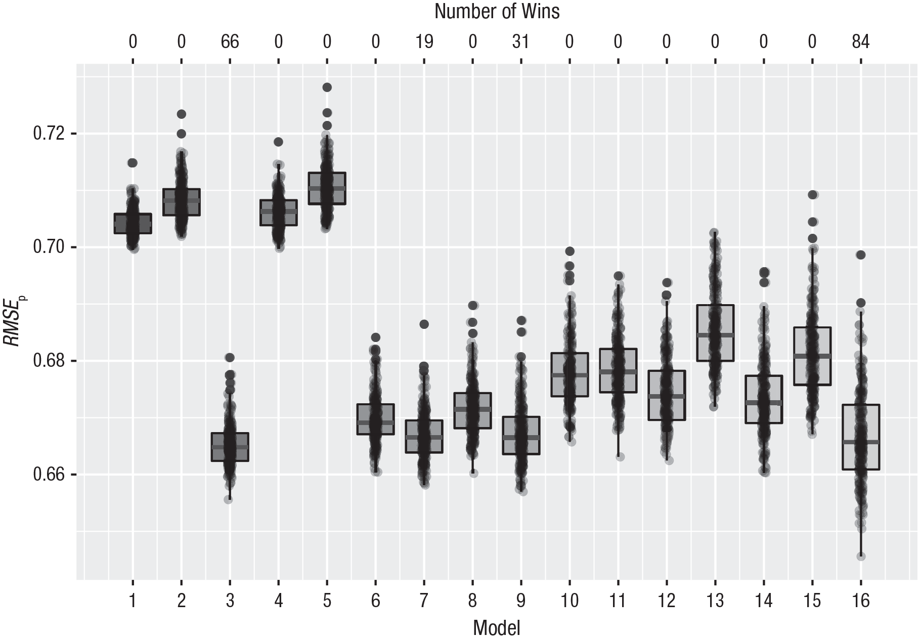
Cross-validation results for the Dutch data on attitudes toward Muslims and multiculturalism. Sixteen different models were formulated (see the text). The vertical axis represents the root mean square error of prediction (RMSE_p). The number of wins is represented at the top of the graph. See Figure 1 for an explanation of the conventions used in the boxplots.

In this case, cross-validation provides quite a bit of information. Although the model with the three-way interaction wins most often, the gain in prediction accuracy is very small. A model with only a main effect of national identification performs equally well and might, just because of its simplicity, be the preferred model.

In this case, we can also use a standard approach of fitting a series of regression models and looking at the change in explained variance and corresponding test statistics. We present this analysis in the Supplemental Material. One problematic aspect of this procedure is that not all models are nested, and therefore not all models can be compared with statistical tests. Furthermore, many p values are computed, which raises the question of how to correct for multiple comparisons. These issues, which also arise in stepwise procedures, are known to be problematic. Finally, this analysis requires distributional assumptions for the residuals. The diagnostic plots question the validity of these assumptions.

Example 4: logistic regression

Hastie and Tibshirani (1990) reported data on the presence or absence of kyphosis, a postoperative spinal deformity. For this example, the predictor variable is the age of the patient in months, and we model the relationship between kyphosis and age using a logistic regression. Therefore, let π(x_i) = p(Y_i = 1|x_i) denote the conditional probability of having kyphosis given age x. The logistic regression model with a linear effect of age on the log odds of kyphosis can be written as

\log (\frac{π (x_{i})}{1 - π (x_{i})}) = a + x_{i} b .

We compare the predictive power of this model with that of a model including only the intercept (i.e., a model in which age does not predict kyphosis) and a model that also includes a quadratic term:

\log (\frac{π (x_{i})}{1 - π (x_{i})}) = a + x_{i} b_{1} + x_{i}^{2} b_{2} .

We repeatedly estimate the model parameters in the calibration sets and then make predictions in the validation sets. These predictions are in the form of probabilities ${\hat{x}}_{j}$ ). Using this prediction in our loss function gives

R M S E_{p} = \sqrt{\frac{1}{N_{V}} \sum_{j = 1}^{N_{V}} {(y_{j} - \hat{π} (x_{j}))}^{2}},

with y_j ∈ {0,1}, which is known as the Brier score.

The data are available in the gam package (Hastie, 2018), in which the response variable is a string variable. In the following code, we first recode the response variable to a 0,1 variable, where 1 indicates presence of kyphosis. We then define three logistic regression models, an intercept-only model, a logistic regression with age as predictor and a logistic regression with age and age-squared as predictors. Finally, the cross-validation function for a logistic regression is called:

library(gam)

data(kyphosis)

kyphosis[,1] = as.numeric(kyphosis[,1] == “present”)

models = vector(mode = “list”, length = 3)

models[[1]] = Kyphosis ~ 1

models[[2]] = Kyphosis ~ Age

models[[3]] = Kyphosis ~ poly(Age,2)

output = xval.glm(data = kyphosis, models, glm.family = binomial)

The results of the cross-validation are shown in the left panel of Figure 6. It is clear that the quadratic polynomial of age gives the best predictions. The right panel of Figure 6 shows the quadratic model fitted on all the data. This is a single-peaked curve; first the probability goes up, and later it goes down. Nowhere does the probability become larger than .5, so for every person, the model predicts the absence of kyphosis. For patients around the age of 100 months, the probability of kyphosis is about .40.

Fig. 6.

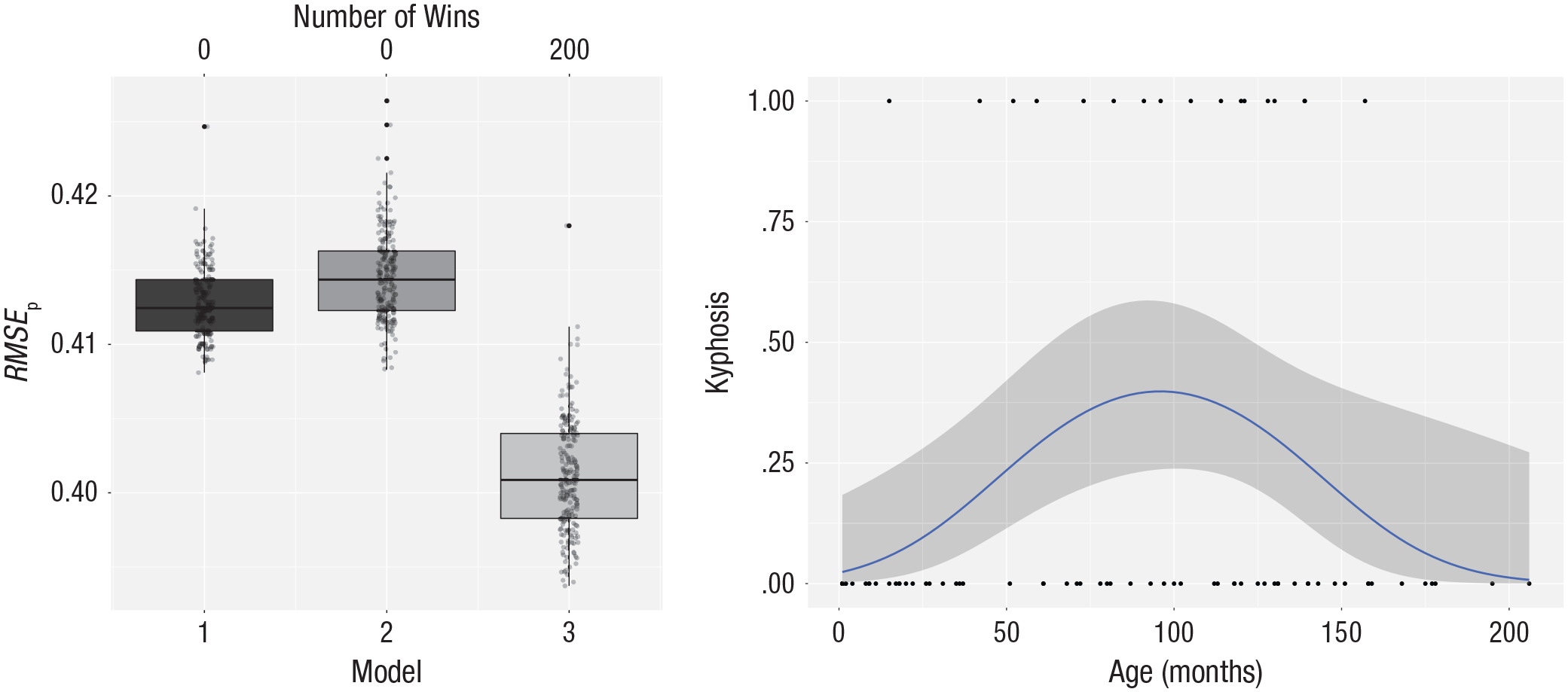
Results for the kyphosis data. The left panel shows the cross-validation results for three logistic models predicting kyphosis from age: Model 1 makes predictions based on an intercept-only model, Model 2 includes age as a predictor, and Model 3 is based on a quadratic function of age. The vertical axis represents the root mean square error of prediction (RMSE_p). The number of wins is represented at the top of the graph. See Figure 1 for an explanation of the conventions used in the boxplots. The right panel shows a scatterplot of the relation between age and the presence of kyphosis. The smooth blue line is the logistic regression line from the model that best fits all the data, and the gray band around this line shows the uncertainty in the predictions (in the unlikely case that all assumptions are met, it represents the 95% confidence interval).

Example 5: changing the loss function

The default way to compute prediction error in our xval.glm function is by the root mean square error of prediction. As shown in the previous subsection, for logistic regression this equals the Brier score. In some situations, one might be interested in another loss function. For linear models, for example, one might be interested in the average absolute error. For logistic regression, one might be interested in the misclassification rate or the cross-validated deviance.

If another loss function should be employed, one first has to define it. This function must have two arguments, the observed responses (y) and the predictions (preds). The function for the average absolute loss is defined in R as

absloss = function(y,preds){mean(abs(y - preds))}

With this function, we can run the four models for the aggression data again with the following adapted call:

output = xval.glm(data = agdat, models, loss = absloss)

Now prediction error is defined as the average absolute error. The results of these four models are portrayed in Figure 7. The quadratic model still provides the best results, although in this case the intercept-only and linear models are closer to the winner than before.

Fig. 7.

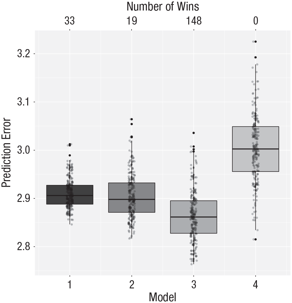
Cross-validation results for the aggression data with mean absolute error as the loss function. Model 1 makes predictions based on the overall mean, Model 2 makes predictions based on a first-order polynomial (i.e., linear model) of aggression, Model 3 uses a second-order polynomial, and Model 4 uses a third-order polynomial. The vertical axis represents the prediction error (“PE” in the xvalglms package), as measured by the mean absolute error. The number of wins is represented at the top of the graph. See Figure 1 for an explanation of the conventions used in the boxplots.

In the Supplemental Material, we also show examples in which we change the loss function in the logistic regression for the kyphosis data from the Brier score to the cross-validated deviance and the misclassification rate. The cross-validated deviance gives results similar to those for the Brier score, whereas the misclassification rate completely changes the conclusions, thus demonstrating the importance of the loss function for the results. The misclassification rate is insensitive to differences in probabilities, whereas the Brier score and the deviance are sensitive to such differences. The analysis using the misclassification rate indicates that age does not have an influence on the presence of kyphosis and that no child will develop kyphosis. The analysis using the Brier score as the loss function indicates that the probability of kyphosis is smaller than .5 for every child, but also that 40% of the treated children around the age of 100 months will develop kyphosis. The main question for the surgeon, then, is whether or not this is an acceptable risk.

Another consideration in the choice of the loss function is the goal of the analysis. Is the goal to classify new patients, or is it to obtain better insight about the relationships between the variables (i.e., to advance theory)? In the first case, one should use the misclassification rate as measure of predictive performance; in the second case, it is better to use a more sensitive measure.

Example 6: comparing the predictive power of two theories

Pollack, VanEpps, and Hayes (2012) investigated the effect of economic stress on intentions to disengage from entrepreneurial activities. The participants in this study were 262 members of a networking group for small-business owners who responded to an online survey about the recent performance of their business and their emotional and cognitive responses to the economic climate.

The participants were asked a series of questions about how they felt their business was doing. Their responses were used to create an index of economic stress (estress; higher scores reflect greater stress). They were also asked to rate the extent to which they had various feelings related to their business, such as feeling discouraged, hopeless, worthless, and the like. An aggregation of these ratings was used to quantify business-related depressed affect (affect; higher scores reflect more depressed affect). Another measure was entrepreneurial self-efficacy (ese), which indexed participants’ confidence in their ability to successfully engage in various entrepreneurship-related tasks, such as setting and meeting goals, creating new products, managing risk, and making decisions. Finally, they were also asked a set of questions to quantify their intentions to withdraw from entrepreneurship in the next year (withdraw; higher scores indicate greater withdrawal intentions). Moreover, we have a set of covariates: sex (0 = female, 1 = male), age (in years), and tenure (length of time in business).

For these data, there are two theories. The first theory is that economic stress has an influence on withdrawal intentions but that this effect is mediated by business-related depressed affect. When we take the covariates into account, this theory leads to a regression model with withdraw as the response and estress, affect, sex, age, and tenure as predictors. The second theory is that economic stress is not at all related to withdrawal intentions and that withdrawal intentions are just an effect of individual differences. That is, more confident persons have less depressed affect and therefore lower intentions to withdraw. When we take the covariates into account, this theory leads to a regression model with withdraw as the response and ese, affect, sex, age, and tenure as predictors.

The two theories lead to two regression models that are not nested. That is, these models are hard to compare using statistical tests such as, for example, the likelihood ratio test. It is, however, quite easy to compare the two theories using cross-validation. This can be done using the following code:

library(foreign)

ecdata = read.spss(“estress.sav”, to.data.frame = TRUE)

models = vector(mode = “list”, length = 2)

models[[1]] = withdraw ~ tenure + estress + affect + sex + age

models[[2]] = withdraw ~ tenure + affect + sex + age + ese

output = xval.glm(data = ecdata, models)

The results are shown in Figure 8, which indicates that the second theory leads to more accurate predictions (i.e., the prediction error is lower).

Fig. 8.

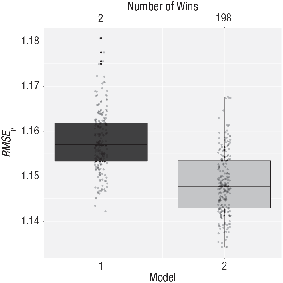
Cross-validation results comparing the predictive power of two theories regarding the relationship between economic stress and intentions to withdraw from entrepreneurship. Theories 1 and 2 (see the text) correspond to Models 1, and 2, respectively. The vertical axis represents the root mean square error of prediction (RMSE_p). The number of wins is represented at the top of the graph. See Figure 1 for an explanation of the conventions used in the boxplots.

Discussion

Lately, there has been an increased interest in an old methodology: cross-validation. The importance of cross-validation for psychological research was recognized quite early (Mosier, 1951). Nevertheless, this method is not often used in psychology, possibly because no simple software tools for implementing it are available. We have developed such a tool in the open-source software R. This R package can be downloaded from the Internet. The function uses K-fold cross-validation and uses many (200) repetitions in order to compare a set of models. Most often the models differ in one term, and the question that is answered is, does this extra term lead to better predictions? The software is built around the family of generalized linear models, which encompass many different analysis methods often used in psychology. The main function (xval.glm) is easily adapted to any other statistical method implemented in R that has an estimation and a prediction function.

We have presented several examples of cross-validation for types of analyses often encountered in psychology. We hope that researchers can adapt the code for their own analyses. We have focused on model selection, in which several models of interest are defined and compared in a repeated K-fold cross-validation procedure. The best model is selected and fitted to all the data, and the result might be used as a prediction tool for the future. Because of the repetitions, our software package yields a distribution of the prediction errors. Note that because the optimal model is selected, there is a risk that these future predictions will be a bit worse compared with the distribution that is obtained in the analysis. This is simply due to regression to the mean, a phenomenon often observed. If an honest measure of prediction error is needed, the model selection is performed as described in the examples, the best model is fitted to the complete data, and finally a good measure of prediction error is obtained using an independent data set (i.e., a separate data set or an independent portion of the original data set). This amounts to doing repeated K-fold cross-validation and testing the selected model on an independent holdout set.

The function we have developed returns boxplots of the prediction error of the different models under consideration, the number of wins of each of the models in the 200 repetitions, and a density curve of the prediction errors for the different models. These density curves sometimes present a better picture of the distribution of prediction errors than the boxplots do. In most of our examples, we had clear winners; that is, the distributions of prediction errors did not show much overlap, and the percentage of wins was largely in favor of one of the models. In our example of moderated regression, results were not as clear, and four competing models were identified. Experience shows that even if one model wins all the time, the distributions of prediction errors may have large overlap, suggesting that for every repeat, one model performs just a little better than the other ones. In such a case, the percentage of wins might be a misleading indicator, and the gain in prediction accuracy should be taken into account. To do so, it is important to relate the measure of prediction error to knowledge about the dependent variable. Is a gain of, for example, 0.5 meaningful in relation to the distribution of the response variable, and would such a gain be noticeable in practice? Sometimes there is considerable overlap in the distributions. For example, the percentages of wins for two models might be 55% and 45%. This means that the data cannot really distinguish between the two models. One choice in such a case would be to favor the more parsimonious model, that is, to conclude that there is not enough evidence that the extra term provides incremental validity. Another choice would be to conclude that there is not enough information to make a choice between the two models. In choosing between two models, one might take into account how easy it is to obtain the extra information required by the more complex one: If it is just a matter of asking a single question, it might be worthwhile to gather and use this information; on the other hand, if a really expensive test (in terms of time or money) is required, it may not be worthwhile to obtain this information in order to improve predictions slightly.

Cross-validation is a resampling technique. Another resampling technique is the bootstrap (Efron & Tibshirani, 1993). The bootstrap is often used to obtain confidence intervals of the parameters of a statistical model, but it can also be used to assess predictive performance, via either of two approaches. In the first approach, many bootstrap samples are drawn from the observed data, and statistical models are fitted to each of them; that is, each of the bootstrap samples is used as the calibration sample, and the observations not in that bootstrap sample (often called the out-of-bag observations) are the validation set. The advantage of this procedure is that the calibration samples are as large as the original sample. Because the bootstrap samples are drawn with replacement, a disadvantage is that only 63.2% of the observations in the original sample are in each bootstrap sample, and this creates bias. The second approach, which was developed to deal with this bias, is called the .632 bootstrap (Efron, 1983; Efron & Tibshirani, 1997). Again, each bootstrap sample is used to calibrate the statistical models, but in this method the validation is performed on the bootstrap sample as well as on the out-of-bag observations. This yields two estimates of prediction error, and the difference between these estimates indicates the optimism of the in-sample approach. The final prediction error is computed as a weighted average of the two measures of prediction error.

A topic we have not discussed is models with tuning parameters, such as modern regression models like the lasso (Tibshirani, 1996). For cross-validation with such a model, one needs to find (a) an optimal value for the penalty parameter and (b) the prediction error for the regression model with the optimal penalty parameter. This can be done with nested cross-validation (Varma & Simon, 2006), in which K-fold cross-validation (inner loop) is performed within K-fold cross-validation (outer loop). More specifically, the data are split in K parts. One part is selected to be the test set, and the others are the training set. K-fold cross-validation is then performed in the training set, by fitting the whole series of models for every possible value of the penalty parameter. The value that gives the smallest prediction error is then used to make predictions in the test set of the outer loop.

There are many ways to do cross-validation. We have focused on repeated K-fold cross-validation, which includes leave-one-out cross-validation. In addition, we have briefly discussed this method’s relationships with the bootstrap and nested cross-validation (see Kohavi, 1995, for a more detailed comparison of cross-validation with the bootstrap). There are other related forms of cross-validation, for which brief descriptions can be found in Steyerberg (2009), Arlot and Celisse (2010), Kuhn and Johnson (2013), and Krstajic, Buturovic, Leahy, and Thomas (2014). Krstajic et al. also discuss the pitfalls and benefits of different cross-validation strategies.

We would like to conclude with the recommendation that cross-validation should be a standard procedure in data analysis, either as a model-selection procedure, as discussed in this article, or as validation of models selected in other ways. Focusing on out-of-sample performance increases the chances that obtained results are replicable (Yarkoni & Westfall, 2017), or as Bokhari and Hubert (2018) declared, “the lack of cross validation can lead to inflated results and spurious conclusions.”

Supplemental Material

De_Rooij_AMPPSOpenPracticesDisclosure-v1.0 – Supplemental material for Cross-Validation: A Method Every Psychologist Should Know

Supplemental material, De_Rooij_AMPPSOpenPracticesDisclosure-v1.0 for Cross-Validation: A Method Every Psychologist Should Know by Mark de Rooij and Wouter Weeda in Advances in Methods and Practices in Psychological Science

Supplemental Material

de_Rooij_Supplemental_Material – Supplemental material for Cross-Validation: A Method Every Psychologist Should Know

Supplemental material, de_Rooij_Supplemental_Material for Cross-Validation: A Method Every Psychologist Should Know by Mark de Rooij and Wouter Weeda in Advances in Methods and Practices in Psychological Science

Footnotes

Acknowledgements

The authors would like to thank two anonymous reviewers for their constructive reviews.

Transparency

Action Editor: Frederick L. Oswald

Editor: Daniel J. Simons

Author Contributions

M. de Rooij initiated an R function and developed several examples. W. Weeda further extended the R function and developed the code into an R package. M. de Rooij wrote the first draft of the manuscript, which the two authors then revised. M. de Rooij finalized the manuscript. M. de Rooij and W. Weeda discussed the reviews and adapted parts of the manuscript and the Supplemental Material in response.

ORCID iDs

Mark de Rooij

Wouter Weeda

Supplemental Material

Additional supporting information can be found at

References

Adams

Wright

Lohr

(1996). Is homophobia associated with homosexual arousal? Journal of Abnormal Psychology, 105, 440–445.

Alexander

D. L. J.

Tropsha

Winkler

D. A.

(2015). Beware of R²: Simple, unambiguous assessment of the prediction accuracy of QSAR and QSPR models. Journal of Chemical Information and Modeling, 55, 1316–1322.

Arlot

Celisse

(2010). A survey of cross-validation procedures for model selection. Statistics Surveys, 4, 40–79.

Bokhari

Hubert

(2018). The lack of cross-validation can lead to inflated results and spurious conclusions: A re-analysis of the MacArthur Violence Risk Assessment Study. Journal of Classification, 35, 147–171.

Breiman

(2001). Statistical modeling: The two cultures. Statistical Science, 16, 199–231.

Browne

M. W.

(2000). Cross-validation methods. Journal of Mathematical Psychology, 44, 108–132.

Chapman

B. P.

Weiss

Duberstein

P. R.

(2016). Statistical learning theory for high dimensional prediction: Application to criterion-keyed scale development. Psychological Methods, 21, 603–620.

Chow

S. L.

(1998). Précis of statistical significance: Rationale, validity, and utility. Behavioral & Brain Sciences, 21, 169–194.

Claudy

(1978). Multiple regression and validity estimation in one sample. Applied Psychological Measurement, 2, 595–607.

10.

Cohen

(1994). The earth is round (p < .05). The American Psychologist, 49, 997–1003.

11.

Cumming

(2014). The new statistics: Why and how. Psychological Science, 25, 7–29.

12.

Darlington

(1968). Multiple regression in psychological research and practice. Psychological Bulletin, 69, 161–182.

13.

Darlington

(1978). Reduced-variance regression. Psycho-logical Bulletin, 85, 1238–1255.

14.

Efron

(1983). Estimating the error rate of a prediction rule: Improvement on cross-validation. Journal of the American Statistical Association, 78, 316–331.

15.

Efron

Tibshirani

(1993). An introduction to the bootstrap. New York, NY: Chapman and Hall.

16.

Efron

Tibshirani

(1997). Improvements on cross-validation: The 632+ bootstrap method. Journal of the American Statistical Association, 92, 548–560.

17.

Fox

(2016). Applied regression analysis & generalized linear models. Thousand Oaks, CA: Sage.

18.

Geisser

(1975). The predictive sample reuse method with applications. Journal of the American Statistical Association, 70, 320–328.

19.

Hagen

R. L.

(1997). In praise of the null-hypothesis statistical test. The American Psychologist, 52, 15–42.

20.

Hagerty

M. R.

Srinivasan

(1991). Comparing the predictive powers of alternative multiple regression models. Psychometrika, 56, 77–85.

21.

Harrell

(2015). Regression modeling strategies: With applications to linear models, logistic and ordinal regression, and survival analysis. New York, NY: Springer.

22.

Hastie

(2018). gam: Generalized Additive Models (R package Version 1.16) [Computer software]. Retrieved from https://cran.r-project.org/web/packages/gam/index.html

23.

Hastie

Tibshirani

(1990). Generalized additive models. New York, NY: Chapman and Hall.

24.

Hastie

Tibshirani

Friedman

(2009). The elements of statistical learning: Data mining, inference, and prediction (2nd ed.). New York, NY: Springer.

25.

Howell

D. C.

(2015). Statistical methods for psychology. Belmont, CA: Thomson Wadsworth.

26.

James

Witten

Hastie

Tibshirani

(2013). An introduction to statistical learning with applications in R. New York, NY: Springer-Verlag.

27.

Kohavi

(1995). A study of cross-validation and bootstrap for accuracy estimation and model selection. Proceedings of the 14th International Joint Conference on Artificial Intelligence (Vol. 2, pp. 1137–1143). San Francisco, CA: Morgan Kaufmann.

28.

Krstajic

Buturovic

L. J.

Leahy

D. E.

Thomas

(2014). Cross-validation pitfalls when selecting and assessing regression and classification models. Journal of Cheminformatics, 6, Article 10. doi:10.1186/1758-2946-6-10

29.

Krueger

(2001). Null hypothesis significance testing: On the survival of a flawed method. The American Psychologist, 56, 16–26.

30.

Kuhn

Johnson

(2013). Applied predictive modeling. New York, NY: Springer.

31.

Lawshe

Schucker

(1959). The relative efficiency of four test weighting methods in multiple prediction. Ed-ucational and Psychological Measurement, 19, 103–114.

32.

Matloff

(2017). Statistical regression and classification: From linear models to machine learning. Boca Raton, FL: CRC Press.

33.

McNeish

D. M.

(2015). Using lasso for predictor selection and to assuage overfitting: A method long overlooked in behavioral sciences. Multivariate Behavioral Research, 50, 471–484.

34.

Mosier

M. W.

(1951). I. Problems and design of cross-validation. Educational and Psychological Measurement, 11, 5–11.

35.

Nickerson

R. S.

(2000). Null hypothesis significance testing: A review of an old and continuing controversy. Psychological Methods, 5, 241–301.

36.

Pollack

J. M.

VanEpps

E. M.

Hayes

A. F.

(2012). The moderating effects of social ties on entrepreneurs’ depressed affect and withdrawal intentions in response to economic stress. Journal of Organizational Behavior, 33, 789–810.

37.

Pruzek

Frederick

(1978). Weighting predictors in linear models: Alternatives to least squares and limitations of equal weights. Psychological Bulletin, 85, 254–266.

38.

R Core Team. (2018). R: A language and environment for statistical computing. Vienna, Austria: R Foundation for Statistical Computing.

39.

Roberts

D. R.

Bahn

Ciuti

Boyce

M. S.

Elith

Guillera-Arroita

. . . Dormann

C. F.

(2016). Cross-validation strategies for data with temporal, spatial, hierarchical, or phylogenetic structure. Ecography, 40, 913–929.

40.

Rozeboom

W. W.

(1960). The fallacy of the null-hypothesis significance test. Psychological Bulletin, 57, 416–428.

41.

Rozeboom

W. W.

(1978). Estimation of cross-validated multiple correlation: A clarification. Psychological Bulletin, 85, 1348–1351.

42.

Rozeboom

W. W.

(1979). Ridge regression: Bonanza or beguilement? Psychological Bulletin, 86, 242–249.

43.

Schmidt

F. L.

(1971). The relative efficiency of regression and simple unit predictor weights in applied differential psychology. Educational and Psychological Measurement, 31, 699–714.

44.

Shmueli

(2010). To explain or to predict. Statistical Science, 25, 289–310.

45.

Steyerberg

E. W.

(2009). Clinical prediction models: A practical approach to development, validation, and updating. New York, NY: Springer.

46.

Stone

(1974). Cross-validatory choice and assessment of statistical predictions [Target article and discussion]. Journal of the Royal Statistical Society: Series B (Methodological), 36, 111–147.

47.

Tibshirani

(1996). Regression shrinkage and selection via the lasso. Journal of the Royal Statistical Society: Series B (Methodological), 58, 267–288.

48.

Tjew-A-Sin

Koole

S. L.

(2018a). Data from paper ‘Terror management in a multicultural society: Effects of mortality salience on attitudes to multiculturalism are moderated by national identification and self-esteem among native Dutch people.’ Journal of Open Psychology Data, 6, Article 5. doi:10.5334/jopd.39

49.

Tjew-A-Sin

Koole

S. L.

(2018b). Terror management in a multicultural society: Effects of mortality salience on attitudes to multiculturalism are moderated by national identification and self-esteem among native Dutch people. Frontiers in Psychology, 9, Article 721. doi:10.3389/fpsyg.2018.00721

50.

Varma

Simon

(2006). Bias in error estimation when using cross-validation for model selection. BMC Bioinformatics, 7, Article 91. doi:10.1186/1471-2105-7-91

51.

Wagenmakers

E.-J.

(2007). A practical solution to the pervasive problem of p values. Psychonomic Bulletin & Review, 14, 779–804.

52.

Wainer

(1976). Estimating coefficients in linear models: It don’t make no nevermind. Psychological Bulletin, 83, 213–217.

53.

Wilcox

R. R.

(2017). Understanding and applying basic statistical methods using R. Hoboken, NJ: John Wiley.

54.

Yarkoni

Westfall

(2017). Choosing prediction over explanation in psychology: Lessons from machine learning. Perspectives on Psychological Science, 12, 1100–1122.

Supplementary Material

Please find the following supplemental material available below.

For Open Access articles published under a Creative Commons License, all supplemental material carries the same license as the article it is associated with.

For non-Open Access articles published, all supplemental material carries a non-exclusive license, and permission requests for re-use of supplemental material or any part of supplemental material shall be sent directly to the copyright owner as specified in the copyright notice associated with the article.

0.00 MB

0.64 MB

1.34 MB